True or Fictitious Flattening? –MEM and the $\theta$ Term –

Abstract

We study the sign problem in lattice field theory with a $\theta$ term. We apply the maximum entropy method (MEM) to flattening phenomenon of the free energy density $f(\theta)$, which originates from the sign problem. In our previous paper, we applied the MEM by employing the Gaussian topological charge distribution $P(Q)$ as mock data. In the present paper, we consider models in which ‘true’ flattening of $f(\theta)$ occurs. These may be regarded as good examples for studying whether the MEM could correctly detect non trivial phase structure.

1 Introduction

A $\theta$ term in QCD is expected to cause interesting dynamics. [1, 2]  Lattice field theory may be a suitable tool as a non perturbative method to study its effect. [3, 4, 5, 6, 7]   However, it suffers from the complex action problem or the sign problem, when a $\theta$ term is included. A conventional technique to avoid the problem is to perform the Fourier transform of the topological charge distribution $P(Q)$, which is calculated with real positive Boltzmann weight, and to calculate the partition function ${\cal Z}(\theta)$. [8, 9]   However, this still causes flattening of the free energy density $f(\theta)$ originated from the error in $P(Q)$. [10, 11]  This phenomenon misleads into a fictitious signal of a first order phase transition. [12]  Some approaches have been tried to overcome the sign problem. [13, 14]  In our previous paper [15] (referred to as (I) hereafter), we applied to this issue the maximum entropy method (MEM), which is suitable to deal with so-called ill-posed problems, where the number of parameters to be determined is much larger than the number of data points. The MEM is based upon Bayes’ theorem. It derives the most probable parameters by utilizing data sets and our knowledge about these parameters in terms of the probability. [16, 17, 18, 19, 20]  The probability distribution, which is called posterior probability, is given by the product of the likelihood function and the prior probability. The latter is represented by the Shannon-Jaynes entropy, which plays an important role to guarantee the uniqueness of the solution, and the former is given by $\chi^{2}$. The task is to explore the image such that the posterior probability is maximized.

In the paper (I), we used the Gaussian $P(Q)$ and tested whether the MEM would be effective, since the Gaussian $P(Q)$ is analytically Fourier-transformed to ${\cal Z}(\theta)$. For the analysis, we used mock data by adding Gaussian noise to $P(Q)$. The results we obtained are the followings; In the case without flattening, the results of the MEM agree with those of the Fourier transform method and thus reproduce the exact results. In the case with flattening, the MEM gives smoother $f(\theta)$ than that of the Fourier transform. Among various default models investigated, some images with the least errors do not show flattening.

If the reason for the disappearance of flattening in the above analysis is the smoothing of the data, which is the characteristic of the parameter inference such as the maximal likelihood method, one may wonder if the MEM may not be a suitable method for detecting singular behaviors such as a phase transition. In order to investigate this issue, we study whether the MEM would be applicable to ‘true’ flattening of $f(\theta)$ or singular behaviors like a first order phase transition occurring at a finite value of $\theta(\neq\pi)$. By ‘true’, it is meant that flattening is not originated from the error of $P(Q)$ but occurs due to the data themselves. For this purpose, we consider a simple model based on mock data. It is a model which consists of the Gaussian $P(Q)$ except at $Q=0$. For $Q=0$, a constant is added to the Gaussian $P(Q)$. This additional contribution at $Q=0$ causes the flattening behavior in the large $\theta$ region ($\theta\leq\pi$). We apply the MEM to this model and study whether true flattening would be properly reproduced.

Although this model develops true flattening, it does not reveal the singularity in $f(\theta)$ at finite value of $\theta(\neq\pi)$. In order to study such a singular behavior mimicking a first order phase transition, we consider a model which utilizes $P(Q)$ obtained by the inverse Fourier transform of a singular $f(\theta)$. In order for the singularity and flattening to be compatible in such a model, obtained $P(Q)$ oscillates and could take negative values for large values of $Q$. Although $P(Q)$ looses the physical meaning as the topological charge distribution for their negative values, we regard this as a mathematical model to study the singular behavior in terms of the MEM.

We apply the MEM to these models and study (i) whether true flattening would be properly reproduced and (ii) how the errors in $P(Q)$ are related with the results of the MEM and the numerical Fourier transform method. Although these models are simple, we expect that this analysis would serve to obtain knowledge if the MEM could be utilized to study the phase structure, when it were applied to other models suffering from the sign problem, say, finite density QCD.

This paper is organized as follows. In the following section, we give an overview of the origin of flattening and a sketch of the MEM. A model developing true flattening is also introduced. In $\S$ 3, the MEM is applied to this model. In $\S$ 4, another model developing a singular behavior is introduced and analyzed.  A summary is given in $\S$ 5.

2 MEM and a model

2.1 Flattening of $f(\theta)$

Let us briefly explain flattening of $f(\theta)$. The partition function ${\cal Z}(\theta)$ can be obtained by Fourier-transforming the topological charge distribution $P(Q)$, which is calculated with real positive Boltzmann weight.

$${\cal Z}(\theta)=\frac{\int[d\bar{z}dz]e^{-S+i\theta\hat{Q}(\bar{z},z)}}{\int[d\bar{z}dz]e^{-S}}\equiv\sum_{Q}e^{i\theta Q}P(Q),$$ (1)

where

$$P(Q)\equiv\frac{\int[d\bar{z}dz]_{Q}e^{-S}}{\int d\bar{z}dze^{-S}}.$$ (2)

The measure $[d\bar{z}dz]_{Q}$ in Eq. (2) represents that the integral is restricted to configurations of the field $z$ with the topological charge $Q$, and $S$ denotes an action.

The distribution $P(Q)$ obtained from Monte Carlo simulations can be decomposed into two parts, a true value ${\tilde{P}}(Q)$ and an error of $P(Q)$. When the error at $Q=0$ dominates, the free energy density becomes

$$f(\theta) = -\frac{1}{V}\log{\cal Z}(\theta)\approx-\frac{1}{V}\log\bigl{\{}\sum_{Q}{\tilde{P}}(Q)e^{i\theta Q}+\delta P(0)\bigr{\}}$$ (3)

$$= -\frac{1}{V}\log\bigl{\{}e^{-V{\tilde{f}}(\theta)}+\delta P(0)\bigr{\}},$$

where ${\tilde{f}}(\theta)$ is the true free energy density and $\delta P(0)$ is the error at $Q=0$. The value of $e^{-V{\tilde{f}}(\theta)}$ decreases rapidly as the volume $V$ and/or $\theta$ increases. When the magnitude of $e^{-V{\tilde{f}}(\theta)}$ becomes comparable to that of $\delta P(0)$ at $\theta\simeq\theta_{\rm f}$, $f(\theta)$ becomes almost constant, $f(\theta)\simeq{\rm const}$, for $\theta\hskip 3.00003pt\raisebox{1.72218pt}{$>$}\raisebox{-3.01385pt}{$\sim$}\hskip 3.00003pt\theta_{\rm f}$. This abrupt change of the behavior is misleadingly identified as a first order phase transition at $\theta\approx\theta_{\rm f}$. This is (fictitious) flattening phenomenon of $f(\theta)$. The error in $P(Q)$ could also lead to negative values of ${\cal Z}(\theta)$. We refer to this, too, as flattening, because its origin is the same. In the case of a large volume, an exponentially increasing amount of data is needed.

2.2 MEM

In this subsection, we briefly explain the MEM in the context of the $\theta$ term. See (I) for details. Instead of dealing with Eq. (1), we consider

$$P(Q)=\int_{-\pi}^{\pi}d\theta\frac{e^{-i\theta Q}}{2\pi}{\cal Z}(\theta).$$ (4)

The MEM is based on Bayes’ theorem. In order to calculate ${\cal Z}(\theta)$, we maximize the probability

$${\rm prob}({\cal Z}(\theta)|P(Q),I)={\rm prob}({\cal Z}(\theta)|I)\frac{{\rm prob}(P(Q)|{\cal Z}(\theta),I)}{{\rm prob}(P(Q)|I)},$$ (5)

where ${\rm prob}(A)$ is the probability that an event $A$ occurs, and ${\rm prob}(A|B)$ is the conditional probability that $A$ occurs under the condition that $B$ occurs.

The likelihood function ${\rm prob}(P(Q)|{\cal Z}(\theta),I)$ is given by

$${\rm prob}(P(Q)|{\cal Z}(\theta),I)=\frac{e^{-\frac{1}{2}\chi^{2}}}{X_{L}},$$ (6)

where $X_{L}$ is a normalization constant, and $\chi^{2}$ is represented by

$$\chi^{2}\equiv\sum_{Q,Q^{\prime}}(P^{({\cal Z})}(Q)-{\bar{P}}(Q))C^{-1}_{Q,Q^{\prime}}(P^{({\cal Z})}(Q^{\prime})-{\bar{P}}(Q^{\prime})).$$ (7)

Here, $P^{({\cal Z})}(Q)$ is constructed from ${\cal Z}(\theta)$ through Eq. (4), and ${\bar{P}}(Q)$ denotes the average of a data set $\{P(Q)\}$;

$${\bar{P}}(Q)=\frac{1}{N_{d}}\sum_{l=1}^{N_{d}}P^{(l)}(Q),$$ (8)

where $N_{d}$ represents the number of sets of data. The matrix $C^{-1}$ represents the inverse covariance matrix obtained by the data set $\{P(Q)\}$.

The prior probability ${\rm prob}({\cal Z}(\theta)|I)$ is represented in terms of the entropy $S$ as

$${\rm prob}({\cal Z}(\theta)|I,\alpha)=\frac{e^{\alpha S}}{X_{S}(\alpha)},$$ (9)

where $\alpha$ is a real positive parameter and $X_{S}(\alpha)$ denotes an $\alpha$-dependent normalization constant. With regard to $S$, the Shannon-Jaynes entropy is employed:

$$S=\int^{\pi}_{-\pi}d\theta\biggl{[}{\cal Z}(\theta)-m(\theta)-{\cal Z}(\theta)\log\frac{{\cal Z}(\theta)}{m(\theta)}\biggr{]},$$ (10)

where $m(\theta)$ is called the ‘default model’. The posterior probability thus amounts to

$${\rm prob}({\cal Z}(\theta)|P(Q),I,\alpha,m)=\frac{e^{-\frac{1}{2}\chi^{2}+\alpha S}}{X_{L}X_{S}(\alpha)},$$ (11)

where it is explicitly shown that $\alpha$ and $m$ are regarded as new prior knowledge in ${\rm prob}({\cal Z}(\theta)|P(Q),I,\alpha,m)$.

For the information $I$, we impose the criterion

$${\cal Z}(\theta)>0$$ (12)

so that ${\rm prob}({\cal Z}(\theta)\leq 0|I,m)=0$.

We employ the following procedure for the analysis. [16, 20]  Details are given in (I).

1. Maximizing $W$ to obtain ${\cal Z}^{(\alpha)}(\theta)$ for a fixed $\alpha$:

   In order to find the image in functional space of ${\cal Z}(\theta)$ for a given $\alpha$, we maximize

   $$W\equiv-\frac{1}{2}\chi^{2}+\alpha S$$ (13)

   so that

   $$\frac{\delta}{\delta{\cal Z}(\theta)}(-\frac{1}{2}\chi^{2}+\alpha S)\Bigm{|}_{{\cal Z}={{\cal Z}^{(\alpha)}}}=0.$$ (14)

   The parameter $\alpha$ plays the role determining the relative weights of $S$.

   In the numerical analysis, the continuous function ${\cal Z}(\theta)$ is discretized;
   ${\cal Z}(\theta)\to{\cal Z}(\theta_{n})\equiv{\cal Z}_{n}$. The integral over $\theta$ in Eq. (4) is converted to the finite summation over $\theta$;

   $$P_{j}=\left\{\begin{array}[]{ll}\displaystyle{\sum_{n=1}^{N_{\theta}}\frac{1}{2\pi}{\cal Z}_{n}}\;\;\;\;\;\;\;(j=1)\\ \displaystyle{\sum_{n=1}^{N_{\theta}}\frac{\cos\theta_{n}j}{\pi}{\cal Z}_{n}}\;(\mbox{otherwise})\end{array}\right\}\equiv\sum_{n=1}^{N_{\theta}}K_{jn}{\cal Z}_{n},$$ (17)

   where $j=1,2,\cdots,N_{q}$ and $n=1,2,\cdots,N_{\theta}$. Note that $P_{j}$ denotes $P(Q)$ at $Q=j-1$ and $N_{q}<N_{\theta}$. Here we used the fact that $P(Q)$ and ${\cal Z}(\theta)$ are even functions of $Q$ and $\theta$, respectively.

2. Averaging ${\cal Z}^{(\alpha)}_{n}$:

   The $\alpha$-independent final image, denoted as ${\hat{\cal Z}}_{n}$ or ${\hat{\cal Z}}(\theta)$, can be calculated by averaging the image ${\cal Z}^{(\alpha)}_{n}$ according to the probability.

   $${\hat{\cal Z}}_{n}=\int d\alpha~{}{\rm prob}(\alpha|P(Q),I,m){\cal Z}^{(\alpha)}_{n}.$$ (18)

   The probability ${\rm prob}(\alpha|P(Q),I,m)$ is given by

   $${\rm prob}(\alpha|P(Q),I,m)=\frac{1}{X_{W}}\exp\biggl{\{}\Lambda(\alpha)+W({\cal Z}^{(\alpha)})\biggr{\}},$$ (19)

   where $X_{{\rm W}}$ is a normalization constant, and $\Lambda(\alpha)\equiv\frac{1}{2}\sum_{k}\log\frac{\alpha}{\alpha+\lambda_{k}}$. Here the values $\lambda_{k}$’s are eigenvalues of the real symmetric matrix in $\theta$ space;

   $$\frac{1}{2}\sqrt{{\cal Z}_{m}}\frac{\partial^{2}\chi^{2}}{\partial{\cal Z}_{m}\partial{\cal Z}_{n}}\sqrt{{\cal Z}_{n}}\Bigm{|}_{{\cal Z}={\cal Z}^{(\alpha)}}.$$ (20)

   In averaging over $\alpha$, we determine a range of $\alpha$ so that ${\rm prob}(\alpha|P(Q),I,m)\geq\frac{1}{10}\times{\rm prob}({\hat{\alpha}}|P(Q),I,m)$ holds, where ${\rm prob}(\alpha|P(Q),I,m)$ is maximized at $\alpha={\hat{\alpha}}$.

3. Error estimation [19, 20]:

   The error of the final output image ${\hat{\cal Z}}_{n}$ is calculated based on the uncertainty of the image, which takes into account the correlations of the images ${\hat{\cal Z}}_{n}$ among different values of $n$. [15]

2.3 A model

In (I), we used the Gaussian $P(Q)$ for the MEM analysis. We parameterized the Gaussian $P(Q)$ as

$$P_{\rm G}(Q)\equiv A\exp[-\frac{c}{V}Q^{2}],$$ (21)

where, e.g., in the case of the 2-d U(1) gauge model, $c$ is a constant depending on the inverse coupling constant $\beta$, and $V$ is the lattice volume. Here $V$ is regarded as a parameter and varied in the analysis. The constant $A$ is fixed so that $\sum_{Q}P_{\rm G}(Q)=1$. In order to study the question whether the MEM could be a useful tool for reproducing true flattening, we consider a simple model.

Suppose in some lattice theory that calculated $P(Q)$ were slightly deviated from the Gaussian one only at $Q=0$:

$$P(Q)=P_{\rm G}(Q)+p_{0}\times\delta_{Q0},$$ (22)

where $p_{0}$ is a positive constant and $\delta_{Q0}$ is the Kronecker symbol. The partition function is analytically obtained by use of the Poisson sum formula as

$${\cal Z}_{\rm pois}(\theta)=A^{\prime}\biggl{\{}\sqrt{\frac{\pi V}{c}}\sum_{n=-\infty}^{\infty}\exp\biggl{[}-\frac{V}{4c}(\theta-2\pi n)^{2}\biggr{]}+p_{0}\biggr{\}},$$ (23)

where $A^{\prime}$ is the normalization constant, which is determined so that ${\cal Z}_{\rm pois}(0)=1$. Because the first term in Eq. (23) is monotonically decreasing function of $\theta$, the role of the constant term is to cause a flat distribution at large values of $\theta$ ($\theta\leq\pi$). Let us call this model a flattening model. We use the distributions $P(Q)$, Eq. (22), to generate mock data by adding Gaussian noises to them as described below.

2.4 Mock data

For preparing the mock data, we add noise with the variance of $\delta\times P(Q)$ to $P(Q)$. This is based on the observations in the procedure which was employed to calculate $P(Q)$ in the simulations of models such as the CP^N-1 model. [5]  This turns out to yield a ratio of the error to the data to be almost constant; $|\delta P(Q)/P(Q)|\approx$ const. The parameter $\delta$ directly affects the covariance matrix, and indirectly influences the error $\delta\hat{{\cal Z}}(\theta)$ of the image, which is the uncertainty of the image. As done in (I), $\delta$ is mainly fixed to 1/400. In order to investigate the effects of $\delta$ on the final image, we also use its smaller values.

A set of data consists of $P(Q)$ with the errors for $Q=0$ to $N_{q}-1$. Employing $N_{d}$ such sets of data, we calculate the covariance matrices in Eq.(7) with the jackknife method as

$$C_{Q,Q^{\prime}}=\frac{1}{N_{d}(N_{d}-1)}\sum_{l=1}^{N_{d}}(P^{(l)}(Q)-{\bar{P}}(Q))(P^{(l)}(Q^{\prime})-{\bar{P}}(Q^{\prime})),$$ (24)

where $P^{(l)}(Q)$ denotes the $l$-th data of the topological charge distribution and ${\bar{P}}(Q)$ is the average Eq.(8). The inverse covariance matrix is calculated with precision that the product of the covariance matrix and its inverse has off-diagonal elements at most ${\cal O}(10^{-23})$. We take $N_{d}=30$ as in (I).

The number of degrees of freedom in $\theta$ space, $N_{\theta}$, is taken to be larger than that of the topological charge $N_{q}$: $N_{\theta}$ is set to be 28. [15]  The number $N_{q}$ is chosen so as to satisfy $P(Q)\geq 10^{-20}$ and to satisfy the quality of the covariance matrix described above. It varies depending on which type of model is used and on $V$. Note that in order to reproduce ${\cal Z}(\theta)$ which ranges many orders, the analysis must be performed with quadruple precision. In order to find a unique solution in the huge configuration space of the image, we employ the singular value decomposition.

As to the default model $m(\theta)$ in Eq.(10), we study various cases: (i) $m(\theta)=$ const. and (ii) $m(\theta)=\exp(-\frac{\ln 10}{\pi^{2}}\gamma\theta^{2})$. In the case of (i), we show the results of $m(\theta)=1.0$. The case (ii) is the Gaussian default, where the parameter $\gamma$ is varied in the analysis.

In the next section, we investigate the following questions: (i) Does the MEM reproduce true flattening? (ii) How does the final image of the partition function depend on $p_{0}$ as well as on the magnitude of the error in $P(Q)$?

3 Results

3.1 Flattening model

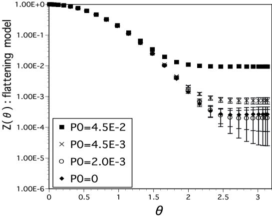
Figure 1: Partition function ${\cal Z}(\theta)$ calculated by numerical Fourier transform for $V=50$. Data for $P(Q)$ in Eq. (22) are used with $p_{0}=4.5\times 10^{-2}$, $4.5\times 10^{-3}$, $2.0\times 10^{-3}$ and $0$. Here, $\delta=1/400$. Clear flattening is observed in each case. The result for $p_{0}=0$ looks similar to that for $2.0\times 10^{-3}$. The latter indicates somewhat smaller errors than the former.

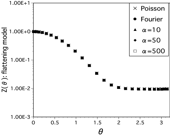
Figure 2: ${\cal Z}^{(\alpha)}(\theta)$ obtained in the procedure 1, Eq. (14), for various values of $\alpha$ in the flattening model. Here, $V=50$, $p_{0}=4.5\times 10^{-2}$ and $\delta=1/400$. The default model is chosen to be the constant $m(\theta)=1.0$.

When noise is added, the partition function for Eq. (22) in the flattening model is given by

$${\cal Z}(\theta)=\frac{\bigl{\{}\sum_{Q}P_{\rm G}(Q)e^{i\theta Q}+p_{0}+\sum_{Q}\delta P(Q)e^{i\theta Q}\bigr{\}}}{B},$$ (25)

where $B=\sum_{Q}\bigl{\{}P_{\rm G}(Q)+p_{0}\delta_{Q0}+\delta P(Q)\bigr{\}}$. Figure 1 displays the behavior of ${\cal Z}(\theta)$ calculated by the numerical Fourier transform of Eq. (22) for $V=50$ and for various values of $p_{0}$; $p_{0}=4.5\times 10^{-2}$, $4.5\times 10^{-3}$ and $2.0\times 10^{-3}$. The parameter $c$ in Eq. (21) is fixed to 7.42 throughout the paper. The parameter $\delta$ is chosen to be $1/400$.

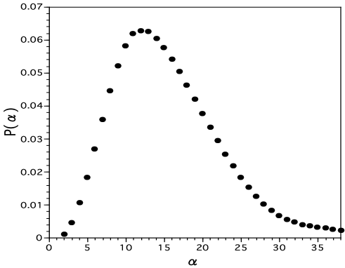
Figure 3: Probability ${\rm prob}(\alpha|P(Q),I,m)\equiv P(\alpha)$ for $V=50$, $p_{0}=4.5\times 10^{-2}$ and $\delta=1/400$ in the flattening model. The default model is chosen to be the constant $m(\theta)=1.0$.

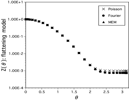
Figure 4: ${\cal Z}(\theta)$ for $V=50$, $p_{0}=4.5\times 10^{-3}$ and $\delta=1/400$ in the flattening model. The default model is chosen to be the constant $m(\theta)=1.0$. Error bars are also displayed but invisible.

Figiure 1 also displays ${\cal Z}(\theta)$ for $p_{0}=0$, which was studied in (I) in detail. Clear flattening is observed in each case. Note that the behavior of ${\cal Z}(\theta)$ and its error are similar for the $p_{0}=2.0\times 10^{-3}$ and $p_{0}=0$ cases. In order to understand what the origin of these flattening is, let us investigate Eq. (25) briefly: When $p_{0}$ is so chosen that for small values of $\theta$, the first term dominates in the numerator, while for large values of $\theta$, the constant term dominates, the resultant ${\cal Z}(\theta)$ behaves like the partition function with flattening. For the latter case, Eq. (25) is approximated by a constant

$${\cal Z}(\theta)\approx\frac{p_{0}}{B}.$$ (26)

For $V=50$ and $p_{0}=4.5\times 10^{-2}$ , $B$ is numerically estimated as 4.45 and thus

$${\cal Z}(\theta)\approx\frac{4.5\times 10^{-2}}{4.45}=1.0\times 10^{-2}.$$ (27)

For other choice of $p_{0}$, $4.5\times 10^{-3}$ and $2.0\times 10^{-3}$, $p_{0}/B$ becomes $1.0\times 10^{-3}$ and $4.5\times 10^{-4}$, respectively. These values agree with those of flattening observed in Fig. 1, and we thus find that these flattening are not caused by the error in $P(Q)$ but are due to the additional term in Eq. (22). On the other hand, to flattening for the $p_{0}=0$ case in Fig. 1, Eq. (26) does not apply obviously. What is observed is not caused by the constant term but comes from the error in $P(Q)$ as described in section 2.1. The former type of flattening is true flattening, because its origin lies in data of $P(Q)$, while the latter ($p_{0}=0$) is fictitious one, because it comes from the error in $P(Q)$.

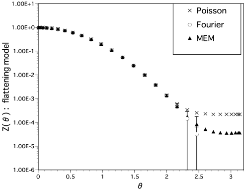
Figure 5: ${\cal Z}(\theta)$ for $V=50$, $p_{0}=1.0\times 10^{-3}$ and $\delta=1/400$ in the flattening model. The default model is chosen to be the constant $m(\theta)=1.0$. Error bars are also displayed but invisible for the MEM results. The Fourier method yields negative values for ${\cal Z}(\theta)$ at $\theta\geq 2.5$.

Table 1: The final image ${\hat{\cal Z}}(\theta)$ in the flattening model at $\theta=2.32$ and $\theta=3.07$ for various values of $p_{0}$. The default model is chosen to be $m(\theta)=1.0$. The exact values ${\cal Z}_{\rm pois}(\theta)$ are also listed. The results of the Fourier method are denoted as ${\cal Z}_{\rm four}$.

$p_{0}$	${\cal Z}_{\rm pois}(2.32)$		${\cal Z}_{\rm four}(2.32)$		$\hat{{\cal Z}}(2.32)$
4.5$\times 10^{-2}$	9.	801$\times 10^{-3}$	9.	6(1)$\times 10^{-3}$	9.	66(1)$\times 10^{-3}$
4.5$\times 10^{-3}$	1.	094$\times 10^{-3}$	9.	1(1.5)$\times 10^{-4}$	8.	99(2)$\times 10^{-4}$
1.0$\times 10^{-3}$	3.	342$\times 10^{-4}$	1.	5(1.5)$\times 10^{-4}$	1.	78(8)$\times 10^{-6}$

$p_{0}$	${\cal Z}_{\rm pois}(3.07)$		${\cal Z}_{\rm four}(3.07)$		$\hat{{\cal Z}}(3.07)$
4.5$\times 10^{-2}$	9.	686$\times 10^{-1}$	9.	5(2)$\times 10^{-3}$	9.	521(2)$\times 10^{-3}$
4.5$\times 10^{-3}$	9.	772$\times 10^{-4}$	7.	5(1.7)$\times 10^{-4}$	7.	410(6)$\times 10^{-4}$
1.0$\times 10^{-3}$	2.	174$\times 10^{-4}$	-1.	5(18.0)$\times 10^{-5}$	3.	6(2)$\times 10^{-6}$

Having distinguished two kinds of flattening, we investigate whether the MEM can properly reproduce the true one. We employ the case for $p_{0}=4.5\times 10^{-2}$, as an example. Figure 2 displays ${\cal Z}^{(\alpha)}(\theta)$, which is calculated by Eq. (14), for various values of $\alpha$. The default model is chosen to be the constant, $m(\theta)=1.0$. We find that ${\cal Z}^{(\alpha)}(\theta)$ are independent of the values of $\alpha$. They show clear flattening in agreement with the result of the Fourier transform and also with that of the Poisson sum formula, Eq. (23).

In order to calculate the final image of the partition function, we need the probability ${\rm prob}(\alpha|P(Q),I,m)$ as shown in Eq. (18). For $m(\theta)=1.0$, ${\rm prob}(\alpha|P(Q),I,m)$ is plotted in Fig. 3. A peak of ${\rm prob}(\alpha|P(Q),I,m)$ is located at $\alpha\approx 12$. The integration to obtain the final image ${\hat{\cal Z}}(\theta)$ thus becomes trivially simple because of the fact that ${\cal Z}^{(\alpha)}(\theta)$ is independent of $\alpha$ in the relevant range for the integration of the procedure 2. Thus ${\hat{\cal Z}}(\theta)$ agrees with ${\cal Z}^{(\alpha)}(\theta)$ in Fig. 2, and the MEM yields true flattening. Note that this situation is unchanged when the Gaussian default model is used, where $\gamma$ is varied between 0.1 and 3.0.

With other choice of the value of $p_{0}$, we repeat the same procedure. For $p_{0}=4.5\times 10^{-3}$, the MEM yields true flattening for the final image ${\hat{\cal Z}}(\theta)$ as plotted in Fig. 4. The errors are also included but invisible in the figure. The result of the MEM agrees with the behavior of the exact partition function (Poisson). For smaller values of $p_{0}$, however, flattening is not reproduced correctly. This is displayed in Fig. 5 for $p_{0}=1.0\times 10^{-3}$; although ${\hat{\cal Z}}(\theta)$ in the MEM flattens for large values of $\theta$, its height is about 4 times smaller than the exact one (Poisson). This analysis shows that there is a critical value of $p_{0}$ above which the MEM is effective, and it is found that $p_{0}$ $\approx 2.0\times 10^{-3}$ in the present case. This critical value is associated with the magnitude of the error in $P(Q)$ or $\delta$. This will be discussed later. The result of the Fourier method, ${\cal Z}_{\rm four}(\theta)$, is also shown as a comparison in Fig. 5. Here, ${\cal Z}_{\rm four}(\theta)$ receives large errors for $2.3\hskip 3.00003pt\raisebox{1.72218pt}{$<$}\raisebox{-3.01385pt}{$\sim$}\hskip 3.00003pt\theta\hskip 3.00003pt\raisebox{1.72218pt}{$<$}\raisebox{-3.01385pt}{$\sim$}\hskip 3.00003pt2.5$. For $\theta\hskip 3.00003pt\raisebox{1.72218pt}{$>$}\raisebox{-3.01385pt}{$\sim$}\hskip 3.00003pt2.5$, ${\cal Z}_{\rm four}(\theta)$ takes negative values and are not plotted in the figure. Table 1 displays the numerical values of ${\hat{\cal Z}}(\theta)$ at two typical values of $\theta$, 2.32 as an intermediate region and 3.07 as the one near $\pi$, for three values of $p_{0}$. The exact values ${\cal Z}_{\rm pois}(\theta)$ and ${\cal Z}_{\rm four}(\theta)$ are also listed.

3.2 $\delta$ dependence

In the model discussed above, the applicability of the MEM is deeply associated with the magnitude of the error in $P(Q)$. In order to investigate this aspect, we vary the value of $\delta$, which controls the magnitude of the error in the mock data. Although it would not be realistic to use data with too small error corresponding to huge amount of statistics, it would still be meaningful to investigate the limitations of the MEM analysis. This is beneficial of using mock data.

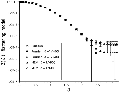
Figure 6: ${\cal Z}(\theta)$ in the flattening model obtained by the numerical Fourier transform and the MEM for $V=50$, $p_{0}=1.0\times 10^{-3}$. The value of $\delta$ is chosen to be $1/400$ and $1/600$ for a comparison. Note that ${\cal Z}_{\rm four}(\theta)$ takes negative values for $\theta\geq 2.5$ in the case $\delta=1/400$ and thus these data are not shown. Error bars for ${\cal Z}_{\rm four}(\theta)$ with $\delta=1/600$ are large, while those of the MEM are invisible.

For the flattening model, we fix the value of $p_{0}$ and vary that of $\delta$. Let us take an example of $p_{0}=1.0\times 10^{-3}$, which is about half the critical value of $p_{0}$ for the $\delta=1/400$ case. As already seen in Fig. 5, both of the methods were not effective in reproducing flattening. We vary the value of $\delta$ from 1/400 down to $1.0\times 10^{-4}$. It is found that already for $\delta=1/500$, the MEM reproduces flattening reasonably well. Figure 6 displays the results of the MEM analysis and those of the numerical Fourier transform for $\delta=$ 1/400 and 1/600 as a comparison. The error bars shown in the figure are those of Fourier transform, while those for the MEM are invisible. For $\delta=1/600$, although the errors for the Fourier method are large at $\theta\approx\pi$, the central values of ${\cal Z}_{\rm four}(\theta)$ are approximately equal to those of the MEM, in contrast to the $\delta=1/400$ case where ${\cal Z}_{\rm four}(\theta)$ takes negative values for $\theta\hskip 3.00003pt\raisebox{1.72218pt}{$>$}\raisebox{-3.01385pt}{$\sim$}\hskip 3.00003pt2.5$. At $\theta=3.07$, the relative error of ${\cal Z}_{\rm four}(\theta)$ goes down to 50 $\%$ for $\delta=1.0\times 10^{-3}$ and 4.6 $\%$ for $\delta=1.0\times 10^{-4}$ while it is about 100$\%$ for $\delta=1/600$.

When $p_{0}$ is chosen to be smaller than $1.0\times 10^{-3}$, the MEM can recover correct images by taking smaller value of $\delta$ than 1/600. For a given value of $p_{0}$, the MEM becomes effective in reproducing correct images, when the value of $\delta$ is reduced to the one corresponding to the precision that $\sum_{Q}|\delta P(Q)|\approx p_{0}$. With this precision of data, ${\cal Z}_{\rm four}(\theta)$ still receives much larger errors than those of the MEM.

4 Singular $f(\theta)$ model

4.1 A mathematical model

Although the flattening model develops true flattening, it does not reveal a singularity in $f(\theta)$. In order to study such a singular behavior mimicking a first order phase transition at finite value of $\theta(\neq\pi)$, we consider a model which utilizes $P(Q)$ obtained by the inverse Fourier transform of a singular $f(\theta)$. Consider a partition function

$${\cal Z}(\theta)=\left\{\begin{array}[]{ll}{\cal Z}_{\rm pois}(\theta)&\mbox{($\theta\leq\theta_{\rm f})$}\\ {\cal Z}_{\rm f}&\mbox{$(\theta_{\rm f}<\theta\leq\pi)$, }\end{array}\right.$$ (30)

where ${\cal Z}_{\rm pois}(\theta)$ is the one obtained from the Poisson sum formula Eq. (23) with $p_{0}=0$, and ${\cal Z}_{\rm f}$ is a positive constant ($={\cal Z}_{\rm pois}(\theta_{\rm f})$). This partition function is inverse-Fourier-transformed to obtain $P(Q)$:

$$P(Q)=\frac{1}{\pi}\left[\int_{0}^{\theta_{\rm f}}d\theta{\cal Z}_{\rm pois}(\theta)\cos\theta Q+\int_{\theta_{\rm f}}^{\pi}d\theta{\cal Z}_{\rm f}\cos\theta Q\right].$$ (31)

The singular behavior at $\theta_{\rm f}$ forces $P(Q)$ to oscillate for large values of $Q$, and $P(Q)$ could take negative values in such a region. Although $P(Q)$ looses the physical meaning as a topological charge distribution for their negative values, we regard such a set of data of $P(Q)$ as a mathematical model. What we are concerned with is rather whether the singular behavior of ${\cal Z}(\theta)$ is reproduced.

In the numerical calculation, however, the singularity appears in a approximated way. Also, $P(Q)$ is truncated at an appropriate value of $Q$ satisfying a constraint to keep the precision of the covariance matrix, which was described in the subsection 2.4. As a consequence, we consider the case where only positive $P(Q)$ are used as well as the one where negative contribution is also taken into account. We use the distributions $P(Q)$, Eq. (31), to generate mock data by adding Gaussian noises to them as in the flattening model. We refer to this as singular $f(\theta)$ model.

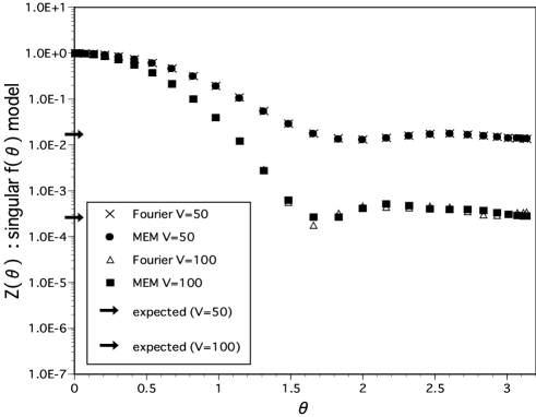
Figure 7: ${\cal Z}(\theta)$ obtained by the numerical Fourier transform and by the MEM for $\theta_{\rm f}=\pi/2$ in the singular $f(\theta)$ model. The upper (lower) one corresponds to $V=50(100)$. The default model is chosen to be the constant $m(\theta)=1.0$. Here, $\delta=1/400$. Error bars are displayed but invisible in both of the methods. Arrows indicate the expected heights of flattening.

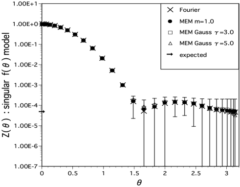
Figure 8: ${\cal Z}(\theta)$ obtained by the numerical Fourier transform and by the MEM for $V=120$ and for $\theta_{\rm f}=\pi/2$ in the singular $f(\theta)$ model. Here, $\delta=1/400$. The results with three different default models are shown. Error bars are of the Fourier method, while those of the MEM are invisible. An arrow indicates the expected height of flattening.

Figure 9: ${\cal Z}(\theta)$ in the singular $f(\theta)$ model obtained by the numerical Fourier transform and the MEM for $V=150$ and $\theta_{f}=\pi/2$. The results for only two values of $\delta$ are plotted: $\delta=1.0\times 10^{-3}$ and $2.0\times 10^{-5}$. The constant default model $m(\theta)=1.0$ is used for the MEM analysis. Error bars of ${\cal Z}_{\rm four}(\theta)$ for $\delta=1.0\times 10^{-3}$ are not shown, while those for the MEM are shown but invisible.

4.2 Results

We are interested in the behavior at $\theta_{\rm f}$ and flattening for $\theta\geq\theta_{\rm f}$. We fix $\theta_{f}$ at an appropriate value, say, $\theta_{\rm f}=\pi/2$ and vary the value of $V$. Figure 7 displays the result of Fourier transform and the final image ${\hat{\cal Z}}(\theta)$ by the MEM analysis for $V=50$ and 100. Here, we truncate $P(Q)$ at some value of $Q$ so that $P(Q)$ becomes positive (Q=7 (12) for $V=50(100)$). For $V=50$, a somewhat acute bend at $\theta_{\rm f}$ and flattening for $\theta\hskip 3.00003pt\raisebox{1.72218pt}{$>$}\raisebox{-3.01385pt}{$\sim$}\hskip 3.00003pt\theta_{\rm f}$ are observed. Here we used $m(\theta)=1.0$ as a default model. The height of flattening is in agreement with the input value of ${\cal Z}_{\rm f}={\cal Z}_{\rm pois}(\pi/2)$. For $V=100$, singular behavior at $\theta_{\rm f}$ becomes clearer, and the height of flattening decreases in agreement with its input value. As $V$ increases, the bend at $\theta_{\rm f}$ becomes more prominent, but the flattening behavior becomes gradually distorted. This is because maximal value of $Q$ used for the analysis is restricted in order to keep the necessary precision of the covariance matrix as stated in subsection 2.4 [15].  These features can also be seen in the case $V=120$ as shown in Fig. 8. Here, the height of flattening agrees with the input value ${\cal Z}_{\rm f}$ indicated by an arrow in the figure. Figure 8 displays default model dependence of the MEM results, where the default models with $m(\theta)=1.0$ and the Gaussian default with $\gamma=3.0$ and $\gamma=5.0$ are chosen. For two values of $\theta$, the values of ${\cal Z}(\theta)$ are listed in Table 2. It is found that the final images of ${\cal Z}(\theta)$ are independent of these default models, and the magnitudes of the errors are almost the same, 1$-$ 3 $\%$. Figure 8 also displays the result of the Fourier method ${\cal Z}_{\rm four}$, where quite large errors are generated for this value of $V$. In the case of $V=120$, $P(Q)$ is truncated at $Q=15$.

As $V$ increases further, the height of flattening decreases, and the image is much more affected by the error of $P(Q)$. Here also, the error of $P(Q)$ puts limitations to the applicability of the MEM as in the flattening model. For $\theta_{\rm f}=\pi/2$, it is found that the MEM cannot be applied already at $V=150$, where the height of flattening of the image ${\hat{\cal Z}}(\theta)$ comes out about one order larger than the input value ${\cal Z}_{\rm f}$, although an acute behavior is still seen at $\theta_{\rm f}$. This will be discussed in the following subsection.

Table 2: $\hat{{\cal Z}}(\theta)$ in the singular $f(\theta)$ model at $\theta=2.32$ and $\theta=3.07$ for various default models. Here, $V=120$.

$\theta$	$\hat{{\cal Z}}_{m=1}$		$\hat{{\cal Z}}_{\gamma=3.0}$		$\hat{{\cal Z}}_{\gamma=5.0}$		${\cal Z}_{\rm four}$
2.32	1.	39(3)$\times 10^{-4}$	1.	47(3)$\times 10^{-4}$	1.	46(3)$\times 10^{-4}$	1.	4 (1.1)$\times 10^{-4}$
3.07	5.	31(5)$\times 10^{-5}$	5.	78(5)$\times 10^{-5}$	4.	65(5)$\times 10^{-5}$	4.	7(15.7)$\times 10^{-5}$

4.3 $\delta$ dependence

By taking advantage of the mock data, we can take very small values of $\delta$. When the errors in $P(Q)$ are much reduced, the Fourier method provides the results with small errors. Let us take an example of $V=150$ in the singular $f(\theta)$ model, to which both of the methods were not effective for $\delta=1/400$ as stated above. We choose $\delta=2.0\times 10^{-5}$ and show the results in Fig. 9. Those for $\delta=1.0\times 10^{-3}$ are also plotted as a comparison. It is found for $\delta=1.0\times 10^{-3}$ that both of the methods are still poor in reproducing flattening, where the error bars for the results of the Fourier method are not shown in the figure, because they are too large. In the case of $\delta=2.0\times 10^{-5}$, on the other hand, a sharp bend at $\theta_{\rm f}=\pi/2$ and flattening at $\theta\geq\pi/2$ are clearly seen. Both of the methods provide consistent results within the errors. Here $P(Q)$ is truncated at $Q=19$ and only positive $P(Q)$ are used.

So far we have presented the results with only positive $P(Q)$ in the singular $f(\theta)$ model. Let us comment about the negative $P(Q)$ in the model. For $V=150$ in Fig. 9, for example, we employed positive $P(Q)$ with $Q=0-19$. For larger values of $Q$, $P(Q)$ oscillates and damps with a maximal amplitude of about $5\times 10^{-8}$. Negative values are also contained like $P(Q)=4.814\times 10^{-8},2.910\times 10^{-8},-3.010\times 10^{-8},-2.140\times 10^{-8},2.696\times 10^{-8},1.731\times 10^{-8}$ and $-2.395\times 10^{-8}$ for $Q=18-24$, respectively. By regarding these values as data and adding Gaussian noise to them, the resultant ${\cal Z}(\theta)$ in the Fourier method differs from that in Fig. 9 by at most 2 $\%$ in the region $\theta_{\rm f}\hskip 3.00003pt\raisebox{1.72218pt}{$<$}\raisebox{-3.01385pt}{$\sim$}\hskip 3.00003pt\theta\leq\pi$, while in the MEM about 6 $\%$ of maximal difference is found at $\theta=1.8(>\theta_{\rm f})$.

5 Summary

We have considered lattice field theory with a $\theta$ term, which suffers from the complex Boltzmann weight problem or the sign problem in numerical simulations. We have applied the MEM to the flattening phenomenon of the free energy originating from the sign problem. In our previous analysis, we studied fictitious flattening of $f(\theta)$. In the present paper, we have investigated whether the MEM could reproduce true flattening. For this, we have used mock data based on the simple models. In the flattening model, the MEM reproduces true flattening. This is different from what was obtained in (I) [15] in the fictitious flattening case, where the MEM could yield monotonically decreasing behaviors of ${\cal Z}(\theta)$ in the whole region of $\theta(0\leq\theta\leq\pi)$. Whether the MEM could reproduce true flattening depends on the magnitude of the error. We have then investigated how the final images are affected by the errors in $P(Q)$ by varying the value of $\delta$. In the flattening model with $\delta=1/400$, when $p_{0}$ is as small as $1.0\times 10^{-3}$, both of the results of the MEM and the Fourier method fail to reproduce flattening. However, as $\delta$ decreases from $1/400$, an immediate improvement has been seen for the MEM. For a given value of $p_{0}$, the MEM becomes effective in reproducing correct images, when the value of $\delta$ is reduced to the one corresponding to the precision that $\sum_{Q}|\delta P(Q)|\approx p_{0}$. With this precision of data, ${\cal Z}_{\rm four}(\theta)$ still receives much larger errors than those of the MEM.

Since the flattening model is free from the singularity, we have considered a model, the singular $f(\theta)$ model, which mimics a first order phase transition at $\theta(<\pi)$. Although this is not a physical model in the strict sense, it would be useful for studying whether the MEM would reproduce the singular behavior. Such behaviors of the free energy at $\theta_{\rm f}$ are approximately reproduced depending on the precision of the data of $P(Q)$. Here also, the MEM is effective when $\sum_{Q}|\delta P(Q)|\hskip 3.00003pt\raisebox{1.72218pt}{$<$}\raisebox{-3.01385pt}{$\sim$}\hskip 3.00003pt{\cal Z}_{\rm f}$.

The errors of the final image in the MEM are calculated from the uncertainty of the image. In the procedure 3 in section 2.2, fluctuations of the image and the correlations among different $\theta$ are properly taken into account according to the probability. However, the smallness of the uncertainty in the MEM may not reflect correct magnitude of the errors. Estimate of such systematic errors is a task to be done in the future. On the other hand, the Fourier method reproduces the results reflecting the errors of $P(Q)$ due to the propagation of the errors. This gives $\sum_{Q}|\delta P(Q)|$ as an estimate of the magnitude of the errors $|\delta{\cal Z}(\theta)|$ for any value of $\theta$, which agree approximately with the results given in sections 3 and 4. In the limit of $\delta P(Q)\rightarrow 0$, therefore, the Fourier method yields correct behavior, whose precision is only affected by the one of computations employed in the analysis; single, double or quadruple precision.

In the present paper, we have concentrated on the issue whether the MEM would be effective with true flattening by employing mock data. A MEM analysis based on real Monte Carlo data will also be necessary. The results of such analysis for the ${\rm CP}^{N-1}$ model will be presented in a forthcoming paper.