Asymptotic behavior of the ghost propagator in SU3 lattice gauge theory

Abstract

We study the asymptotic behavior of the ghost propagator in the quenched SU(3) lattice gauge theory with Wilson action. The study is performed on lattices with a physical volume fixed around 1.6 fm and different lattice spacings: 0.100 fm, 0.070 fm and 0.055 fm. We implement an efficient algorithm for computing the Faddeev-Popov operator on the lattice. We are able to extrapolate the lattice data for the ghost propagator towards the continuum and to show that the extrapolated data on each lattice can be described up to four-loop perturbation theory from 2.0 GeV to 6.0 GeV. The three-loop values are consistent with those extracted from previous perturbative studies of the gluon propagator. However the effective $\Lambda_{\overline{\text{MS}}}$ scale which reproduces the data does depend strongly upon the order of perturbation theory and on the renormalization scheme used in the parametrization. We show how the truncation of the perturbative series can account for the magnitude of the dependency in this energy range. The contribution of non-perturbative corrections will be discussed elsewhere.

1 Introduction

Whereas lattice gauge theory (LGT) has been initially formulated to study gauge-invariant quantities in the non-perturbative regime, it has long been recognized that LGT could be a useful tool for studying gauge-variant quantities such as Green functions, both in the non-perturbative and in the perturbative regimes. The SU(3) gluon propagator in momentum space was first considered [1] to gain some insight into the physics of confinement. Much work was then devoted to the study of its infrared behavior (for a review see [2]). Subsequent studies [3, 4] were focused on the ultraviolet behavior and have been able to compare quantitatively the large momentum dependence of the lattice gluon propagator with perturbative predictions beyond one-loop order. The result for $\Lambda_{\overline{\text{MS}}}$ was found to depend strongly upon the order of the perturbation theory and upon the renormalisation scheme used in the parametrization. This strong dependence raised the question whether the energy windows in these calculations were large enough for perturbative QCD to be a valid approximation.

On the other hand, as shown by Gribov [5], the infrared behavior of the gluon propagator is closely related to the singularity structure of the ghost propagator inferred from the gauge-fixing ambiguities. As is well-known, the Landau gauge, which is presently the only covariant gauge for which there exists effective local gauge-fixing algorithms on the lattice, suffers from these ambiguities. The comprehensive theoretical study by Zwanziger [6] of the Faddeev-Popov operator on the lattice in Landau gauge spurred the first numerical study of the ghost propagator [7] in SU(2) and SU(3) gauge theories. Most subsequent activity has been dedicated to the SU(2) lattice gauge theory in the infrared region, mainly for technical reasons as we shall explain below. There are relatively few numerical studies of the SU(3) ghost propagator which are either more focused on the infrared region and the Gribov copy problem [8, 9, 10] or have only performed a qualitative perturbative description in the quenched approximation [11, 12] and, quite recently, in the unquenched case also [13].

It is important to make the study of the SU(3) ghost propagator in the ultraviolet region more quantitative for comparison purposes with the gluon propagator. Lattice results at small distances may be described by perturbation theory and the independent extraction of the $\Lambda_{\text{QCD}}$ scale from the two propagators would provide a self-consistency test of the analysis and of the lattice approach. It would be particularly significant to confirm or not, from the study of the lattice propagators alone, the need for the non-perturbative power corrections found in the study of the three-gluon coupling on the lattice [14].

The paper is organized as follows. We will begin by recalling in section 2 the method used to relate lattice data for the ghost propagator to its perturbative renormalization description. Then we proceed by exhibiting in section 3 the salient features of our lattice calculation, particularly of our implementation of the Faddeev-Popov operator on the lattice. The following section outlines the general method that we devised previously [3, 4] to eliminate hypercubic artifacts from two-point functions and extrapolate the lattice data towards the continuum. This extrapolation is crucial to succeed in a quantitative description. The results are discussed in section 5 which contains several subsections where the analysis is performed in different renormalization schemes up to four-loop order. In particular the scheme dependence is thoroughly investigated and used to probe the effects of the truncation of the perturbative series. We conclude in section 6 with a comparison of the different methods to compute the $\Lambda_{\text{QCD}}$ scale on the lattice.

2 Renormalization description of the ghost propagator

Let $\Gamma^{(n)}_{B}$ be some gauge-fixed multiplicatively renormalizable one-particle irreducible $n$-point bare Green function defined in euclidean momentum space and in some regularization scheme with cut-off $\Lambda$. Let $s$ denotes some polarization state and kinematical configuration of the external particles contributing to $\Gamma^{(n)}_{B}$. Let $p$ denote a scale transformation on $s$ and $g_{B}$ denote the bare coupling. It is well known that, in any renormalization scheme $R$ defined by some renormalization conditions on state $s$ at the renormalization point $p=\mu$, we have

$$\Gamma^{(n)}_{B}(p,s,g_{B},\Lambda)=Z_{\Gamma,R}(\mu,s,g_{R},\Lambda)\Gamma^{(n)}_{R}(p,s,g_{R},\mu)+{\cal O}(\Lambda^{-1})$$ (1)

where $Z_{\Gamma,R}$ is the renormalization constant in scheme $R$, $\Gamma^{(n)}_{R}$ is the renormalized Green function and $g_{R}(\mu)$ is the renormalized coupling. We omit the dependence on the gauge parameter for simplicity of notation since we will specialize to Landau gauge.

The explicit dependence on $\mu$ drops out of the renormalized Green function $\Gamma^{(n)}_{R}$ at the renormalization point $p=\mu$. It follows that

$$\begin{split}\lim_{\Lambda\rightarrow\infty}\frac{d\ln\left(\Gamma^{(n)}_{B}(\mu,s,g_{B},\Lambda)\right)}{d\ln\mu^{2}}&=\lim_{\Lambda\rightarrow\infty}\frac{d\ln\left(Z_{\Gamma,R}(\mu,s,g_{R},\Lambda)\right)}{d\ln\mu^{2}}+\frac{d\ln\left(\Gamma^{n}_{R}(s,g_{R})\right)}{d\ln\mu^{2}}\\ &\equiv\gamma_{\Gamma,R}(g_{R})+\frac{dg_{R}}{d\ln\mu^{2}}\frac{\partial\ln\Gamma^{n}_{R}}{\partial g_{R}}\end{split}$$ (2)

The arbitrariness in the choice of the renormalization scheme $R$ has prompted attempts at determining the “best” schemes for describing the $q^{2}$-evolution of bare Green functions on the lattice. Clearly it is always possible to find a change of coupling which will be a best approximation of a set of data at a given order of perturbation theory, within some prescribed criteria. Rather than pursuing this route, we will follow the standard wisdom which consists in choosing renormalization conditions appropriate to the continuum quantity under scrutiny.

Momentum substraction schemes have long been used to define renormalization conditions befitted to the description of the renormalization dependence of “physical” quantities. They are defined by setting some of the 2 and 3-point functions to their tree values. In the $\widetilde{\text{MOM}}$ schemes, for these Green functions, Eq. (2) simplifies to

$$\lim_{\Lambda\rightarrow\infty}\frac{d\ln\left(\Gamma^{(n)}_{B}(\mu,s,g_{B},\Lambda)\right)}{d\ln\mu^{2}} =\frac{d\ln(Z_{\Gamma,MOM})}{d\ln\mu^{2}}=\gamma_{\Gamma,MOM}(g_{MOM})$$ (3)

Infinitely many MOM schemes can be defined which differ by the substraction point of the vertices. We have shown in [3] that the $\widetilde{\text{MOMg}}$ scheme defined by substracting the transversal part of the three-gluon vertex at the asymmetric point where one external momentum vanishes, appears to provide a much better estimate of the asymptotic behavior of the gluon propagator in Landau gauge than the $\overline{\text{MS}}$ scheme. For the study of the asymptotic behavior of the ghost propagator in Landau gauge, it seems therefore natural to use a $\widetilde{\text{MOMc}}$ scheme defined by substracting the ghost-gluon vertex at the asymmetric point where the momentum of the external gluon vanishes. Comparison of the two $\widetilde{\text{MOM}}$ schemes should provide us with an estimate of the systematic error entailed in the truncation of the perturbation theory.

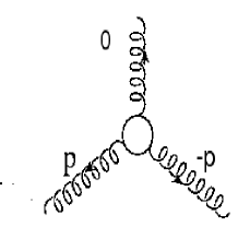
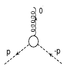
Figure 1: $\widetilde{\text{MOMg}}$ scheme (left) and $\widetilde{\text{MOMc}}$ scheme (right).

The perturbative calculation of the gluon, ghost and quark self-energies and all 3-vertices appearing in the QCD Lagrangian have been done at three-loop order in the $\overline{\text{MS}}$ scheme and in a general covariant gauge at the asymmetric point with one vanishing momentum [15]. These three-loop results allow one to relate the coupling constants of any $\widetilde{\text{MOM}}$-like scheme to the $\overline{\text{MS}}$ scheme at three-loop order. For the $\widetilde{\text{MOMg}}$ and $\widetilde{\text{MOMc}}$ schemes defined above these relations read respectively in Landau gauge and in the quenched approximation ($n_{f}=0$), with $\displaystyle{h=\frac{g^{2}}{16\pi^{2}}}$:

$$\begin{split}h_{\widetilde{\text{MOMg}}}&=h_{\overline{\text{MS}}}+\frac{70}{3}\,h^{2}_{\overline{\text{MS}}}+\left(\frac{516217}{576}-\frac{153}{4}\zeta_{3}\right)h^{3}_{\overline{\text{MS}}}\\ &+\left(\frac{304676635}{6912}-\frac{299961}{64}\zeta_{3}-\frac{81825}{64}\zeta_{5}\right)h^{4}_{\overline{\text{MS}}}\end{split}$$ (4)

$$\begin{split}h_{\widetilde{\text{MOMc}}}&=h_{\overline{\text{MS}}}+\frac{223}{12}\,h^{2}_{\overline{\text{MS}}}+\left(\frac{918819}{1296}-\frac{351}{8}\zeta_{3}\right)h^{3}_{\overline{\text{MS}}}\\ &+\left(\frac{29551181}{864}-\frac{137199}{32}\zeta_{3}-\frac{74295}{64}\zeta_{5}\right)h^{4}_{\overline{\text{MS}}}\end{split}$$ (5)

The very large coefficients of these perturbative expansions explain the difficulties met by the $\overline{\text{MS}}$ scheme to approach asymptotic scaling below 10 GeV.

The recent calculation [16] of the anomalous dimensions in the $\overline{\text{MS}}$ scheme of the gluon and ghost fields at four-loop order, together with the knowledge of the $\beta$-function [17], makes it possible to perform the analysis of the lattice data for the gluon and ghost propagators up to four-loop order also in the $\widetilde{\text{MOMg}}$ and $\widetilde{\text{MOMc}}$ schemes. The numerical coefficients of the $\beta$-function defined as

$$\beta(h)=\frac{dh}{d\ln\mu^{2}}=-\sum_{i=0}^{n}\beta_{i}h^{i+2}+{\cal O}(h^{n+3})$$ (6)

are:

$$\beta_{2}^{\widetilde{\text{MOMg}}}=2412.16,\ \ \beta_{2}^{\widetilde{\text{MOMc}}}=2952.73,\ \beta_{3}^{\widetilde{\text{MOMg}}}=84353.8,\ \beta_{3}^{\widetilde{\text{MOMc}}}=101484.$$ (7)

For completeness we also give the expansion coefficients of the renormalisation constants of the gluon and ghost fields in the MOM schemes with respect to the renormalized coupling of the $\overline{\text{MS}}$ scheme up to four-loop order:

$$\begin{split}\frac{d\ln(Z_{3,MOM})}{d\ln\mu^{2}}&=\frac{13}{2}\,h_{\overline{\text{MS}}}+\frac{3727}{24}\,h^{2}_{\overline{\text{MS}}}+\left(\frac{2127823}{288}-\frac{9747}{16}\zeta_{3}\right)h^{3}_{\overline{\text{MS}}}\\ &+\left(\frac{3011547563}{6912}-\frac{18987543}{256}\zeta_{3}-\frac{1431945}{64}\zeta_{5}\right)h^{4}_{\overline{\text{MS}}}\end{split}$$ (8)

$$\begin{split}\frac{d\ln(\widetilde{Z}_{3,MOM})}{d\ln\mu^{2}}&=\frac{9}{4}\,h_{\overline{\text{MS}}}+\frac{813}{16}\,h^{2}_{\overline{\text{MS}}}+\left(\frac{157303}{64}-\frac{5697}{32}\zeta_{3}\right)h^{3}_{\overline{\text{MS}}}\\ &+\left(\frac{219384137}{1536}-\frac{9207729}{512}\zeta_{3}-\frac{221535}{32}\zeta_{5}\right)h^{4}_{\overline{\text{MS}}}\end{split}$$ (9)

3 Lattice calculation

3.1 Faddeev-Popov operator on the lattice

The ghost propagator is defined on the lattice as

$$G(x-y)\delta^{ab}\equiv\left<\left(M^{-1}\right)^{ab}_{xy}\right>$$ (10)

where the action of the Faddeev-Popov operator $M$ on an arbitrary element $\eta$ of the Lie algebra ${\cal SU}$(N) of the gauge group SU(N), in a Landau gauge fixed configuration, is given by [6]:

$$(M\eta)^{a}(x) =\frac{1}{N}\sum_{\mu}\biggl{\{}G_{\mu}^{ab}(x)\left(\eta^{b}(x+\hat{\mu})-\eta^{b}(x)\right)-(x\leftrightarrow x-\hat{\mu})$$

$$\qquad\qquad+\frac{1}{2}f^{abc}(\eta^{b}(x+\hat{\mu})A_{\mu}^{c}(x)-\eta^{b}(x-\hat{\mu})A_{\mu}^{c}(x-\hat{\mu})\bigr{)}\biggr{\}}$$ (11)

and where, with antihermitian generators $T^{a}$,

$$G_{\mu}^{ab}(x) =\frac{1}{2}\mathsf{Tr}\left(\left\{T^{a},T^{b}\right\}\left(U_{\mu}(x)+U_{\mu}^{\dagger}(x)\right)\right)$$ (12)

$$A_{\mu}^{c}(x) =-\mathsf{Tr}\left(T^{c}\left(U_{\mu}(x)-U_{\mu}^{\dagger}(x)\right)\right)$$ (13)

Most lattice implementations of the Faddeev-Popov operator have followed closely the component-wise Eqs. (3.1-13). But the derivation in [6] shows that the Faddev-Popov operator can also be written as a lattice divergence:

$$M(U)=-\frac{1}{N}\nabla\cdot\widetilde{D}(U)$$ (14)

where the operator $\widetilde{D}$ reads

$$\widetilde{D}_{\mu}(U)\eta(x) =\frac{1}{2}\left(U_{\mu}(x)\eta(x+\hat{\mu})-\eta(x)U_{\mu}(x)+\eta(x+\hat{\mu})U^{\dagger}_{\mu}(x)-U^{\dagger}_{\mu}(x)\eta(x)\right)$$ (15)

Using conversion routines between the Lie algebra and the Lie group, eqs. (14-15) allow for a very efficient lattice implementation, sketched in Table 1, which is based on the fast routines coding the group multiplication law.

 

$$!\ \eta_{in},\ \eta_{out}\ \text{are the ghost fields.}$$

$$!\ U\ \text{is the gauge configuration.}$$

$$\mathrm{type~{}(SUN)}\quad U(*),dU,W,W_{+},W_{-}$$

$$\mathrm{type~{}({\cal SU}N)}\quad\eta_{in}(*),\eta_{out}(*)$$

$$\mathrm{for~{}all~{}x:}$$

$$\quad dU=0.$$

$$\quad W=\eta_{in}(x)$$

$$\quad\mathrm{do}\ \mu=1,\ 4$$

$$\quad\qquad W_{+}=\eta_{in}(x+\hat{\mu})$$

$$\quad\qquad W_{-}=\eta_{in}(x-\hat{\mu})$$

$$\quad\qquad dU=dU+U_{\mu}(x-\hat{\mu})\times W+W\times U_{\mu}(x)$$

$$\quad\qquad\quad\qquad\quad-U_{\mu}(x)\times W_{+}-W_{-}\times U_{\mu}(x-\hat{\mu})$$

$$\quad\mathrm{enddo}$$

$$\quad\eta_{out}(x)=dU-dU^{\dagger}-\frac{1}{N}\mathsf{Tr}(dU-dU^{\dagger})$$

 

Table 1: Pseudo code of our implementation of the Faddeev-Popov operator.

3.2 Inversion of the Faddeev-Popov operator

Constant fields are zero modes of the Faddeev-Popov operator. This operator can be inverted only in the vector subspace $K^{\perp}$ orthogonal to its kernel. If the Faddeev-Popov operator has no other zero modes than constant fields, then the non-zero Fourier modes form a basis of $K^{\perp}$:

$$\eta(x)=\sum_{p\neq 0}c_{p}e^{ip\cdot x}\,,\quad\forall\eta\in K^{\perp}$$ (16)

The standard procedure has been to invert the Faddev-Popov operator with one non-zero Fourier mode as a source

$$S^{a}_{p}(x)=\delta^{ab}e^{ip\cdot x}$$ (17)

and to take the scalar product of $M^{-1}S^{a}_{p}$ with the source:

$$\left(S^{a}_{p}\left|\right.M^{-1}S^{a}_{p}\right) =\sum_{x,y}\left(M^{-1}\right)^{aa}_{xy}e^{-ip\cdot(x-y)}$$ (18)

$$=V\,\widehat{G}(p)$$ (19)

after averaging over the gauge field configurations. This method requires one matrix inversion for each value of the ghost propagator in momentum space. It is suitable only when one is interested in a few values of the ghost propagator.

However, the study of the ultraviolet behavior of the ghost propagator in the continuum requires its calculation at many lattice momenta to control the spacing artifacts, as we shall see in the next section. This can be done very economically by noting that

$$\delta(x,y)=\frac{1}{V}+\frac{1}{V}\sum_{p\neq 0}e^{-ip\cdot(x-y)}$$ (20)

and choosing as source:

$$S^{a}_{0}(x)=\delta^{ab}\left(\delta(x,0)-\frac{1}{V}\right)$$ (21)

The Fourier transform of $M^{-1}S^{a}_{0}$, averaged over the gauge configurations, yields:

$$\sum_{x}e^{-ip\cdot x}\left<M^{-1}S^{a}_{0}\right> =\sum_{x}e^{-ip\cdot x}\left<\left(M^{-1}\right)^{aa}_{x0}\right>-\frac{1}{V}\sum_{x,y}e^{-ip\cdot x}\left<\left(M^{-1}\right)^{aa}_{xy}\right>$$

$$=\sum_{x}e^{-ip\cdot x}G(x)-\frac{1}{V}\sum_{x,y}e^{-ip\cdot x}G(x-y)$$

$$=\widehat{G}(p)-\delta(p)\sum_{x}G(x)$$ (22)

as a consequence of the translation invariance of the ghost propagator. Therefore, with this choice of source, only one matrix inversion followed by one Fourier transformation of the solution is required to get the full ghost propagator on the lattice.

There is of course a price to pay, as can be read off Eq. (22) which lacks the factor $V$ present in Eq. (19). The statistical accuracy with the source $S^{a}_{p}$ is better, especially at high momentum $p$. However the statistical accuracy with the source $S^{a}_{0}$ turns out to be sufficient for our purpose.

There is one final point we want to make and which has never beeen raised to the best of our knowledge. It is mandatory to check, whatever the choice of sources, that rounding errors during the inversion do not destroy the condition that the solution belongs to $K^{\perp}$:

$$\sum_{x}\left(M^{-1}S\right)(x)=0$$ (23)

Indeed, if the zero-mode component of the solution grows beyond some threshold during the inversion of the Faddeev-Popov operator on some gauge configuration, then that component starts to increase exponentially and a sizeable bias is produced in other components as well. We have observed this phenomenon occasionally, about one gauge configuration every few hundreds, when using the implementation of the lattice Faddeev-Popov operator based on Eqs. (3.1-13). But the systematic bias which is induced on the averages over gauge field configurations can be uncomfortably close to those ascribed to Gribov copies.

Another virtue of the algorithm described in Table 1 is its numerical stability which is improved by several orders of magnitude. We have never observed sizeable deviations from Eq. (23) with this algorithm.

3.3 The simulation

We ran simulations of the $SU(3)$ lattice gauge theory with the Wilson action in the quenched approximation on several hypercubic lattices, whose parameters are summarized in Table 2. All lattices have roughly the same physical volume except the $24^{4}$ lattice at $\beta=6.0$ which has been included to check out finite-volume effects.

$\beta$	$V$	$a^{-1}$ (GeV)	# Configurations
$6.0$	$16^{4}$	$1.96$	$1000$
$6.0$	$24^{4}$	$1.96$	$500$
$6.2$	$24^{4}$	$2.75$	$500$
$6.4$	$32^{4}$	$3.66$	$250$

Table 2: Run parameters. The lattice spacings are taken from Table 3 in [18] with a physical unit normalized by $\sqrt{\sigma}=445$ MeV.

The SU(3) gauge configurations were generated using a hybrid algorithm of Cabibbo-Marinari heatbath and Creutz overrelaxation steps. 10000 lattice updates were discarded for thermalization and the configurations were analyzed every 100/200/500 sweeps on the $16^{4}/24^{4}/32^{4}$ lattices.

Landau gauge fixing was carried out by minimizing the functional

$$F_{U}[g]=\text{Re}\sum_{x}\sum_{\mu}\left(1-\frac{1}{N}g(x)U_{\mu}(x)g^{\dagger}(x+\hat{\mu})\right)$$ (24)

by use of a standard overrelaxation algorithm driving the gauge configuration to a local minimum of $F_{U}[g]$. We did not try to reach the fundamental modular region $\Lambda$, defined as the set of absolute minima of $F_{U}[g]$ on all gauge orbits. Indeed there have been numerous studies, in SU(2) [19, 20] and in SU(3) [8, 9], of the effect of Gribov copies on the ghost propagator. The consensus is that noticeable systematic errors, beyond statistical errors, are only found for the smallest $p^{2}$, much smaller than the squared momenta that we used to study the asymptotic behavior of the ghost propagator.

Then the ghost propagator $G(p)$ is extracted from Eq. (22) for all $p\neq 0$. The required matrix inversion, with a conjugate-gradient algorithm without any preconditioning, and the Fourier transform consume in average less than half the computing time of the Landau gauge fixing.

4 Hypercubic artifacts

The ghost propagator $\widehat{G}(p)$ is a scalar invariant on the lattice which means that it is invariant along the orbit $O(p)$ generated by the action of the isometry group $H(4)$ of hypercubic lattices on the discrete momentum $p\equiv\frac{2\pi}{La}\times(n_{1},n_{2},n_{3},n_{4})$ where the $n_{\mu}$’s are integers, $L$ is the lattice size and $a$ the lattice spacing. The general structure of polynomials invariant under a finite group is known from group-invariant theory. Indeed it can be shown that any polynomial function of $p$ which is invariant under the action of $H(4)$ is a polynomial function of the 4 invariants $p^{[n]}=a^{n}\sum_{\mu}p_{\mu}^{n},n=2,4,6,8$ which index the set of orbits.

Our analysis program uses these 4 invariants to average the ghost propagator over the orbits of $H(4)$ to increase the statistical accuracy:

$$a^{2}G_{L}(p^{[2]},p^{[4]},p^{[6]},p^{[8]})=\frac{1}{\|O(p)\|}\sum_{p\in O(p)}\widehat{G}(p)$$ (25)

where $\|O(p)\|$ is the cardinal number of the orbit $O(p)$. By the same token, one should always take the following real source

$$\overline{S}^{a}_{p}(x)=\delta^{ab}\sum_{p\in O(p)}\cos(p\cdot x)$$ (26)

rather than a single complex Fourier mode for studies of the ghost propagator in the infrared region. Indeed, after averaging over the gauge configurations and use of the translational invariance, one gets

$$\left<\left(\overline{S}^{a}_{p}\left|\right.M^{-1}\overline{S}^{a}_{p}\right)\right> =\sum_{p,p^{\prime}\in O(p)}\sum_{x,y}\left<\left(M^{-1}\right)^{aa}_{xy}\right>e^{-ip^{\prime}\cdot x+ip\cdot y}$$

$$=V\|O(p)\|\,a^{2}G_{L}(p^{[2]},p^{[4]},p^{[6]},p^{[8]})$$ (27)

By analogy with the free lattice propagator

$$G_{0}(p)=\frac{1}{\sum_{\mu}\widehat{p}_{\mu}^{2}}=\frac{a^{2}}{p^{[2]}}\left(1+\frac{1}{12}\frac{p^{[4]}}{p^{[2]}}+\cdots\right)\,,\quad\mathrm{where}\quad\widehat{p}_{\mu}=\frac{2}{a}\sin\left(\frac{ap_{\mu}}{2}\right)$$ (28)

it is natural to make the hypothesis that the lattice ghost propagator is a smooth function of the discrete invariants near the continuum limit, when $a\,p_{\mu}\ll 1\,,\forall\mu$,

$$G_{L}(p^{[2]},p^{[4]},p^{[6]},p^{[8]})\approx G_{L}(p^{[2]},0,0,0)+p^{[4]}\frac{\partial G_{L}}{\partial p^{[4]}}(p^{[2]},0,0,0)+\cdots$$ (29)

and $G_{L}(p^{[2]},0,0,0)$ is nothing but the propagator of the continuuum in a finite volume, up to lattice artifacts which do not break $O(4)$ invariance. When several orbits exist with the same $p^{2}$, the simplest method to reduce the hypercubic artifacts is to extrapolate the lattice data towards $G_{L}(p^{[2]},0,0,0)$ by making a linear regression at fixed $p^{2}$ with respect to the invariant $p^{[4]}$ since the other invariants are of higher order in the lattice spacing. The range of validity of this linear approximation can be checked a posteriori from the smoothness of the extrapolated data with respect to $p^{2}$.

Choosing the variables $\widehat{p}_{\mu}$ appropriate to the parametrization of a lattice propagator with periodic boundary conditions provides an independent check of the extrapolation. Indeed we can write as well

$$G_{L}(p^{[2]},p^{[4]},p^{[6]},p^{[8]})\equiv\widehat{G}_{L}(\widehat{p}^{[2]},\widehat{p}^{[4]},\widehat{p}^{[6]},\widehat{p}^{[8]})$$ (30)

with the new invariants, again hierachically suppressed with respect to the lattice spacing,

$$\widehat{p}^{[n]}=a^{n}\sum_{\mu}\widehat{p}_{\mu}^{n}$$ (31)

$G_{L}$ and $\widehat{G}_{L}$ are two different parametrizations of the same lattice data, but near the continuum limit one must also have

$$\widehat{G}_{L}(\widehat{p}^{[2]},\widehat{p}^{[4]},\widehat{p}^{[6]},\widehat{p}^{[8]})\approx\widehat{G}_{L}(\widehat{p}^{[2]},0,0,0)+\widehat{p}^{[4]}\frac{\partial\widehat{G}_{L}}{\partial\widehat{p}^{[4]}}(\widehat{p}^{[2]},0,0,0)+\cdots$$ (32)

where $G_{L}(p^{[2]},0,0,0)$ and $\widehat{G}_{L}(\widehat{p}^{[2]},0,0,0)$ are the same function, the propagator of the continuum , of a different variable (again up to lattice artifacts which do not break $O(4)$ invariance).

If one wants to include in the data analysis the points with a single orbit at fixed $p^{2}$, one must interpolate the slopes extracted from Eqs (29) or (32). This interpolation can be done either numerically or by assuming a functional dependence of the slope with respect to $p^{2}$ based on dimensional arguments. The simplest ansatz is to assume that the slope has the same leading behavior as for a free lattice propagator:

$$\frac{\partial G_{L}}{\partial p^{[4]}}(p^{[2]},0,0,0) =\frac{1}{\left(p^{[2]}\right)^{2}}\left(c_{1}+c_{2}p^{[2]}\right)$$ (33)

The inclusion of $O(4)$-invariant lattice spacing corrections is required to get fits with a reasonable $\chi^{2}$. The quality of such two-parameter fits to the slopes, and the extension of the fitting window in $p^{2}$, supplies still another independent check of the validity of the extrapolations.

We have used Eqs. (29) and (33) to extrapolate our lattice data towards the continuum and determined the range of validity in $p^{2}$ of the extrapolations from the consistency of the different checks within our statistical errors. The errors on the extrapolated points have been computed with the jackknife method. Tables 3 and 4 summarize the cuts that have been applied to the data for the estimation of the systematic errors in the analysis of the next section. We have repeated the analysis of the gluon propagator [4] to study the sensitivity of the results with respect to the window in $p^{2}$ which has been enlarged considerably in our new data. The cuts for the lattice ghost propagator are stronger than for the gluon lattice propagator because the statistical errors of the former are two to three times larger which make the continuum extrapolations less controllable.

$\beta$	$V$	$N_{points}$	$a\,p_{min}$	$a\,p_{max}$	$\chi^{2}$
$6.0$	$16^{4}$	$>10$	$\leq 1.30$	$\leq 1.82$	$\leq 1.4$
$6.2$	$24^{4}$	$>12$	$\leq 1.30$	$\leq 1.82$	$\leq 1.1$
$6.4$	$32^{4}$	$>20$	$\leq 1.40$	$\leq 1.82$	$\leq 1.3$

Table 3: Cuts on the lattice data for the gluon propagator. $[a\,p_{min},a\,p_{max}]$ is the momentum window of a fit in lattice units and $N_{points}$ is the number of data points in that window.

$\beta$	$V$	$N_{points}$	$a\,p_{min}$	$a\,p_{max}$	$\chi^{2}$
$6.0$	$16^{4}$	$>10$	$\leq 1.30$	$\leq 1.57$	$\leq 1.0$
$6.2$	$24^{4}$	$>20$	$\leq 1.30$	$\leq 1.57$	$\leq 1.0$
$6.4$	$32^{4}$	$>20$	$\leq 1.00$	$\leq 1.57$	$\leq 1.0$

Table 4: Cuts on the lattice data for the ghost propagator. Columns have the same meaning as in Table 3.

The number of distinct orbits at each $p^{2}$ increases with the lattice size and, eventually, a linear extrapolation limited to the single invariant $p^{[4]}$ breaks down. However there is a systematic way to include higher-order invariants and to extend the range of validity of the extrapolations. A much more detailed exposition of the controlling of systematic errors is in preparation, since our method has been largely ignored in the litterature where very empirical recipes are still in use.

5 Data analysis

The evolution equation of the renormalization constants of the gluon or ghost fields in a MOM scheme, with respect to the coupling constant $h$ in an arbitrary scheme $R$ (the index $R$ is omitted but understood everywhere), can be written generically up to four-loop order:

$$\frac{d\ln(Z_{\Gamma,MOM})}{d\ln\mu^{2}}=\overline{\gamma}_{0}h+\overline{\gamma}_{1}h^{2}+\overline{\gamma}_{2}h^{3}+\overline{\gamma}_{3}h^{4}$$ (34)

and the perturbative integration of Eq. (34) yields, to the same order,

$$\begin{split}\ln\left(\frac{Z_{\Gamma,MOM}}{Z_{0}}\right)&=\log(h)\,\frac{\overline{\gamma}_{0}}{\beta_{0}}+h\,\frac{\left(\beta_{0}\,\overline{\gamma}_{1}-\beta_{1}\,\overline{\gamma}_{0}\right)}{\beta_{0}^{2}}\\ &+h^{2}\,\frac{\left(\beta_{0}^{2}\,\overline{\gamma}_{2}-\beta_{0}\,\beta_{1}\,\overline{\gamma}_{1}-(\beta_{0}\,\beta_{2}-\beta_{1}^{2})\,\overline{\gamma}_{0}\right)}{2\beta_{0}^{3}}\\ &+h^{3}\,\bigl{(}\beta_{0}^{3}\,\overline{\gamma}_{3}-\beta_{0}^{2}\,\beta_{1}\,\overline{\gamma}_{2}+(\beta_{0}\,\beta_{1}^{2}-\beta_{0}^{2}\,\beta_{2})\,\overline{\gamma}_{1}\\ &\qquad+(-\beta_{0}^{2}\,\beta_{3}+2\,\beta_{0}\,\beta_{1}\,\beta_{2}-\beta_{1}^{3})\,\overline{\gamma}_{0}\bigr{)}\frac{1}{3\beta_{0}^{4}}\end{split}$$ (35)

with the standard four-loop formula for the running coupling

$$\begin{split}h(t)&=\frac{1}{\beta_{0}t}\left(1-\frac{\beta_{1}}{\beta_{0}^{2}}\frac{\log(t)}{t}+\frac{\beta_{1}^{2}}{\beta_{0}^{4}}\frac{1}{t^{2}}\left(\left(\log(t)-\frac{1}{2}\right)^{2}+\frac{\beta_{2}\beta_{0}}{\beta_{1}^{2}}-\frac{5}{4}\right)\right)\\ &+\frac{1}{(\beta_{0}t)^{4}}\left(\frac{\beta_{3}}{2\beta_{0}}+\frac{1}{2}\left(\frac{\beta_{1}}{\beta_{0}}\right)^{3}\left(-2\log^{3}(t)+5\log^{2}(t)+\left(4-6\frac{\beta_{2}\beta_{0}}{\beta_{1}^{2}}\right)\log(t)-1\right)\right)\end{split}$$ (36)

and $\displaystyle{t=\log\left(\frac{\mu^{2}}{\Lambda^{2}}\right)}$.

We now consider in turn the three renormalization schemes $\overline{\text{MS}}$, $\widetilde{\text{MOMg}}$ and $\widetilde{\text{MOMc}}$ and fit the two parameters of Eqs. (35) and (36) to our extrapolated lattice data. Figure 2 illustrates the typical quality of such fits.

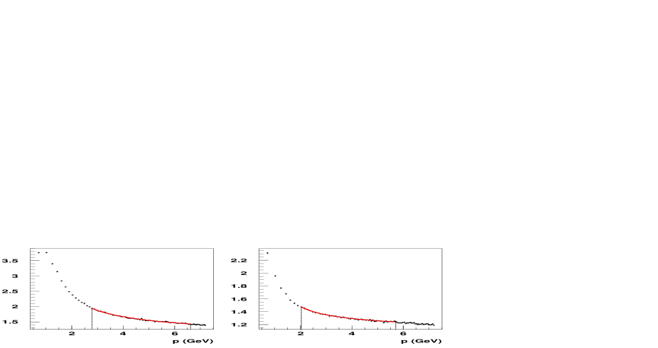
Figure 2: Extrapolated lattice data at $\beta=6.4$ for $Z_{3}$ (left) and $\widetilde{Z}_{3}$ (right). The solid line is the fit at four-loop order in the $\overline{\text{MS}}$ scheme. The vertical dotted lines delimit the window of each fit.

5.1 $\overline{\text{MS}}$ scheme

The analysis in the $\overline{\text{MS}}$ scheme is summarized in Table 5. The statistical error is at the level of 1% for the gluon propagator and 2-3% for the ghost propagator, whereas the systematic error due to the extrapolations is around 3-5% and 5-10% respectively. The values of $\Lambda_{\overline{\text{MS}}}$ extracted from the gluon and the ghost propagators are consistent within these errors and within each order of perturbation theory.

$\beta$	$L$	$a$pmin	$a\Lambda^{(2)}_{\overline{\text{MS}},gluon}$	$\chi^{2}$	$a\Lambda^{(3)}_{\overline{\text{MS}},gluon}$	$\chi^{2}$	$a\Lambda^{(4)}_{\overline{\text{MS}},gluon}$	$\chi^{2}$
6.0	16	1.111	0.336(3)${}^{+8~{}}_{-4~{}}$	1.3	0.265(3)${}^{+6~{}}_{-2~{}}$	1.0	0.225(2)${}^{+4~{}}_{-2~{}}$	1.1
	24	1.111	0.332(3)${}^{+8~{}}_{-12}$	0.6	0.262(3)${}^{+6~{}}_{-8~{}}$	0.5	0.222(2)${}^{+5~{}}_{-8~{}}$	0.6
6.2	24	0.907	0.240(2)${}^{+6~{}}_{-9~{}}$	0.8	0.185(2)${}^{+6~{}}_{-10}$	0.8	0.158(2)${}^{+4~{}}_{-7~{}}$	0.8
6.4	32	0.760	0.171(2)${}^{+10}_{-11}$	1.4	0.130(2)${}^{+12}_{-11}$	1.4	0.112(1)${}^{+9~{}}_{-8~{}}$	1.4
$\beta$	$L$	$a$pmin	$a\Lambda^{(2)}_{\overline{\text{MS}},ghost}$	$\chi^{2}$	$a\Lambda^{(3)}_{\overline{\text{MS}},ghost}$	$\chi^{2}$	$a\Lambda^{(4)}_{\overline{\text{MS}},ghost}$	$\chi^{2}$
6.0	16	1.039	0.354(7)${}^{+23}_{-13}$	0.5	0.281(6)${}^{+17}_{-8~{}}$	0.5	0.235(5)${}^{+15}_{-7~{}}$	0.5
	24	0.785	0.325(6)${}^{+13}_{-20}$	0.2	0.259(5)${}^{+10}_{-18}$	0.2	0.217(4)${}^{+8~{}}_{-13}$	0.2
6.2	24	0.693	0.254(4)${}^{+20}_{-20}$	0.4	0.200(3)${}^{+10}_{-23}$	0.4	0.169(3)${}^{+12}_{-13}$	0.4
6.4	32	0.555	0.193(2)${}^{+22}_{-14}$	0.8	0.150(2)${}^{+15}_{-14}$	0.8	0.128(2)${}^{+13}_{-11}$	0.8

Table 5: Fits of $\Lambda_{\overline{\text{MS}}}$ from the gluon and ghost lattice propagators. The error in parenthesis is the statistical error corresponding to a window $[a\,p_{min},a\,p_{max}]$ with the $a\,p_{min}$ quoted in the Table and the upper bound for $a\,p_{max}$ quoted in Tables 3 and 4 respectively.

However, the three-loop and four-loop values, which are displayed in Table 6 with the physical units of Table 2, clearly confirm our previous result [3] that we are still far from asymptoticity in that scheme.

$\beta$	$\Lambda^{(3)}_{\overline{\text{MS}},gluon}$	$\Lambda^{(3)}_{\overline{\text{MS}},ghost}$	$\Lambda^{(4)}_{\overline{\text{MS}},gluon}$	$\Lambda^{(4)}_{\overline{\text{MS}},ghost}$
6.0	$519(6)^{+12}_{-4~{}}$	$551(12)^{+33}_{-16}$	$441(4)^{+8~{}}_{-4~{}}$	$461(10)^{+29}_{-14}$
6.2	$509(6)^{+17}_{-27}$	$550(8)^{+27}_{-63}~{}$	$435(6)^{+11}_{-19}$	$465(8)^{+33}_{-36}~{}$
6.4	$476(7)^{+44}_{-40}$	$549(7)^{+55}_{-51}~{}$	$410(4)^{+33}_{-29}$	$468(7)^{+48}_{-40}~{}$

Table 6: Three-loop and four-loop physical values of $\Lambda_{\overline{\text{MS}}}$ in MeV extracted from Table 5.

5.2 $\widetilde{\text{MOMg}}$ scheme

Table 7, which summarizes the analysis in the $\widetilde{\text{MOMg}}$ scheme, shows that, at the lower $\beta$’s, we were not able to describe both lattice propagators at four-loop order with reasonable cuts and $\chi^{2}$. This could be interpreted as an hint that perturbation theory has some problems of convergence beyond three-loop order below 3-4 GeV.

$\beta$	$L$	$a$pmin	$a\Lambda^{(2)}_{\widetilde{\text{MOMg}},gluon}$	$\chi^{2}$	$a\Lambda^{(3)}_{\widetilde{\text{MOMg}},gluon}$	$\chi^{2}$	$a\Lambda^{(4)}_{\widetilde{\text{MOMg}},gluon}$	$\chi^{2}$
6.0	16	1.039	0.551(3)${}^{+8~{}}_{-8~{}}$	1.0	0.477(3)${}^{+5~{}}_{-8~{}}$	1.2	—	—
	24	1.014	0.536(4)${}^{+14}_{-19}$	0.9	0.464(3)${}^{+10}_{-11}$	0.9	—	—
6.2	24	0.693	0.396(2)${}^{+19}_{-12}$	1.0	0.336(2)${}^{+8~{}}_{-15}$	0.9	—	—
6.4	32	0.555	0.292(1)${}^{+15}_{-14}$	1.3	0.246(1)${}^{+7~{}}_{-20}$	1.4	0.253(3)${}^{+5~{}}_{-3~{}}$	1.6
$\beta$	$L$	$a$pmin	$a\Lambda^{(2)}_{\widetilde{\text{MOMg}},ghost}$	$\chi^{2}$	$a\Lambda^{(3)}_{\widetilde{\text{MOMg}},ghost}$	$\chi^{2}$	$a\Lambda^{(4)}_{\widetilde{\text{MOMg}},ghost}$	$\chi^{2}$
6.0	16	1.039	0.660(40)${}^{+24}_{-29}$	0.4	0.475(12)${}^{+29}_{-24}$	0.5	—	—
	24	1.014	0.559(22)${}^{+25}_{-20}$	0.2	0.438(12)${}^{+14}_{-25}$	0.2	0.408(17)${}^{+20}_{-18}$	0.9
6.2	24	0.693	0.455(11)${}^{+9~{}}_{-17}$	0.3	0.342(5)${}^{+27}_{-34}~{}$	0.6	0.348(8)${}^{+23}_{-17}~{}$	1.0
6.4	32	0.555	0.333(4)${}^{+36}_{-26}~{}$	1.2	0.261(3)${}^{+33}_{-28}~{}$	0.9	0.279(7)${}^{+14}_{-30}~{}$	0.8

Table 7: Fits of $\Lambda_{\widetilde{\text{MOMg}}}$ from the gluon and ghost lattice propagators. The notations are the same as in Table 5.

If we select the three-loop result as the best perturbative estimate of $\Lambda_{\widetilde{\text{MOMg}}}$ and convert it to the $\overline{\text{MS}}$ scheme with the asymptotic one-loop formula, $\Lambda_{\overline{\text{MS}}}=0.346\,\Lambda_{\widetilde{\text{MOMg}}}$, then we get the physical values quoted in Table 8 which agree completely with previous values [4].

$\beta$	$\Lambda^{(3)}_{\overline{\text{MS}},gluon}$	$\Lambda^{(3)}_{\overline{\text{MS}},ghost}$
6.0	324(2)${}^{+2~{}}_{-5~{}}$	322(8)${}^{+20}_{-16}$
6.2	320(2)${}^{+8~{}}_{-14}$	326(5)${}^{+26}_{-33}$
6.4	312(1)${}^{+9~{}}_{-25}$	331(4)${}^{+42}_{-35}$

Table 8: Three-loop physical values of $\Lambda_{\overline{\text{MS}}}$ in MeV extracted from Table 7.

5.3 $\widetilde{\text{MOMc}}$ scheme

The results of the analysis in the $\widetilde{\text{MOMc}}$ scheme are displayed in Table 9. We still find that the three-loop and four-loop values of $\Lambda^{(3)}_{\widetilde{\text{MOMc}}}$ are very much the same both for the gluon propagator and for the ghost propagator. Thus the perturbative series seems again to become asymptotic at three-loop order in that scheme.

$\beta$	$L$	$a$pmin	$a\Lambda^{(2)}_{\widetilde{\text{MOMc}},gluon}$	$\chi^{2}$	$a\Lambda^{(3)}_{\widetilde{\text{MOMc}},gluon}$	$\chi^{2}$	$a\Lambda^{(4)}_{\widetilde{\text{MOMc}},gluon}$	$\chi^{2}$
6.0	16	1.178	0.482(6)	1.3	0.408(3)${}^{+4~{}}_{-4~{}}~{}$	1.0	—	—
	24	1.111	0.468(5)${}^{+6~{}}_{-5~{}}~{}$	0.5	0.394(3)${}^{+11}_{-6~{}}~{}$	0.8	0.411(7)${}^{+3~{}}_{-2~{}}~{}$	1.1
6.2	24	0.907	0.345(3)${}^{+17}_{-10}~{}$	0.9	0.288(2)${}^{+5~{}}_{-6~{}}~{}$	0.9	0.292(3)${}^{+8~{}}_{-5~{}}~{}$	0.8
6.4	32	0.589	0.255(1)${}^{+12}_{-15}~{}$	1.5	0.205(1)${}^{+11}_{-7~{}}~{}$	1.6	0.212(1)${}^{+9~{}}_{-17}~{}$	1.6
$\beta$	$L$	$a$pmin	$a\Lambda^{(2)}_{\widetilde{\text{MOMc}},ghost}$	$\chi^{2}$	$a\Lambda^{(3)}_{\widetilde{\text{MOMc}},ghost}$	$\chi^{2}$	$a\Lambda^{(4)}_{\widetilde{\text{MOMc}},ghost}$	$\chi^{2}$
6.0	16	0.962	0.489(6)${}^{+10}_{-6~{}}~{}$	0.8	0.437(11)${}^{+6~{}}_{-2~{}}$	0.4	—	—
	24	1.047	0.459(6)${}^{+15}_{-15}~{}$	0.5	0.408(8)${}^{+6~{}}_{-5~{}}~{}$	0.5	0.398(14)${}^{+13}_{-20}$	0.3
6.2	24	0.740	0.367(7)${}^{+21}_{-33}~{}$	0.4	0.308(7)${}^{+9~{}}_{-16}~{}$	0.2	0.303(9)${}^{+7~{}}_{-14}~{}$	0.2
6.4	32	0.589	0.280(5)${}^{+28}_{-23}~{}$	0.6	0.225(5)${}^{+18}_{-13}~{}$	0.6	0.224(5)${}^{+15}_{-16}~{}$	0.6

Table 9: Fits of $\Lambda_{\widetilde{\text{MOMc}}}$ from the gluon and ghost lattice propagators. The notations are the same as in Table 5.

Selecting the three-loop result as the best perturbative estimate of $\Lambda_{\widetilde{\text{MOMc}}}$ and converting it to the $\overline{\text{MS}}$ scheme with the asymptotic formula, $\Lambda_{\overline{\text{MS}}}=0.429\,\Lambda_{\widetilde{\text{MOMc}}}$, we get the physical values quoted in Table 10.

$\beta$	$\Lambda^{(3)}_{\overline{\text{MS}},gluon}$	$\Lambda^{(3)}_{\overline{\text{MS}},ghost}$
6.0	345(3)${}^{+4~{}}_{-4~{}}$	369(9)${}^{+3~{}}_{-2~{}}$
6.2	341(2)${}^{+6~{}}_{-7~{}}$	364(8)${}^{+11}_{-19}$
6.4	323(2)${}^{+17}_{-11}$	354(8)${}^{+28}_{-20}$

Table 10: Three-loop physical values of $\Lambda_{\overline{\text{MS}}}$ in MeV extracted from Table 9.

5.4 Scheme dependence

The puzzling feature of Tables 6, 8 and 10 is the rather large dependence of the $\Lambda_{\text{QCD}}$ scale upon the loop-order and the renormalisation scheme whereas, within any scheme, the values from the ghost and gluon propagators are rather consistent at each loop order and pretty independent of the lattice spacing.

Let us consider again the evolution equation of the renormalisation constants of the gluon or ghost fields in a MOM scheme, with respect to the coupling $h_{R}$ in an arbitrary scheme $R$. We have

$$\frac{d\ln(Z_{\Gamma,MOM})}{d\ln\mu^{2}}=\overline{\gamma}_{R}(h_{R})=-\frac{1}{2}\frac{d\ln(Z_{\Gamma,MOM})}{d\ln\Lambda_{R}}$$ (37)

where $\Lambda_{R}$ is the scale in scheme $R$. If we truncate the perturbative expansion at order $n$

$$\ln\left(\frac{Z_{\Gamma,MOM}}{Z_{0}}\right)=c_{R,0}\ln(h_{R})+\sum_{k=1}^{n-1}c_{R,k}h_{R}^{k}$$ (38)

the change in the effective scale $\Lambda^{(n)}_{R}$, or equivalently, the change in the coupling $h_{R}$, induced by adding the contribution at order $n+1$ is typically

$$\frac{\Delta\Lambda^{(n)}_{R}}{\Lambda^{(n)}_{R}}\approx-\frac{c_{R,n}h_{R}^{n}}{2\gamma_{R}(h_{R})}$$ (39)

Now the dependence of the effective scale $\Lambda_{R}$ upon the coupling $h_{R}$ is given up to order 4

$$2\ln\Lambda^{(4)}_{R}=\ln\mu^{2}-\frac{1}{\beta_{0}h_{R}}-\frac{\beta_{1}}{\beta_{0}^{2}}\ln(\beta_{0}h_{R})-\frac{\beta_{0}\beta_{2}-\beta_{1}^{2}}{\beta_{0}^{3}}h_{R}-\frac{\beta_{0}^{2}\beta_{3}-2\beta_{0}\beta_{1}\beta_{2}+\beta_{1}^{3}}{2\beta_{0}^{4}}h_{R}^{2}$$ (40)

and, denoting the coefficient of order $h_{R}^{n-2}$ in that equation by $-\rho_{R,n-1}$, the effective scales which describe a same coupling at order $n$ and $n+1$ are related by

$$\ln\frac{\Lambda^{(n+1)}_{R}}{\Lambda^{(n)}_{R}}\equiv-\frac{1}{2}\rho_{R,n-1}h_{R}^{n-1}$$ (41)

Combining Eqs. (39) and (41) gives the relation between the effective scales which describe the renormalisation constants of the gluon or ghost fields in a MOM scheme at order $n$ and $n+1$

$$\frac{\Lambda^{(n+1)}_{R}}{\Lambda^{(n)}_{R}}=\exp-\frac{1}{2}\left(\rho_{R,n-1}+\frac{c_{R,n}h_{R}}{\gamma_{R}(h_{R})}\right)h_{R}^{n-1}$$ (42)

Figure 3 displays the behavior of this ratio for the gluon and ghost propagators in the three schemes as a function of the momentum $p$ for $n=2$ and $n=3$. The couplings are taken from the fits at $\beta=6.4$.

Figure 3: $\frac{\Lambda^{(n+1)}_{R}}{\Lambda^{(n)}_{R}}$ for $n=2$ (dashed lines) and $n=3$ (solid lines), for the gluon propagator in the $\overline{\text{MS}}$ scheme (a), $\widetilde{\text{MOMg}}$ scheme (c) and $\widetilde{\text{MOMc}}$ scheme (e), and for the ghost propagator in the $\overline{\text{MS}}$ scheme (b), $\widetilde{\text{MOMg}}$ scheme (d) and $\widetilde{\text{MOMc}}$ scheme (f).

There is a pretty good qualitative agreement with Tables 6, 8 and 10, which confirms the overall consistency with perturbation theory of the lattice data for the gluon and ghost propagators within any renormalization scheme.

The scheme dependence of the $\Lambda_{\text{QCD}}$ scale can also be analyzed with Eq. (40):

$$\frac{\Lambda^{(n)}_{R_{2}}}{\Lambda^{(n)}_{R_{1}}}=\exp\left\{\frac{1}{2\beta_{0}}\left(\frac{1}{h_{R_{1}}}-\frac{1}{h_{R_{2}}}\right)+\frac{\beta_{1}}{2\beta_{0}^{2}}\ln\frac{h_{R_{1}}}{h_{R_{2}}}+\cdots\right\}$$ (43)

Figure 4 shows the behavior of the ratios $\frac{\Lambda^{(n)}_{\overline{\text{MS}}}}{\Lambda^{(n)}_{\widetilde{\text{MOMg}}}}$ and $\frac{\Lambda^{(n)}_{\widetilde{\text{MOMc}}}}{\Lambda^{(n)}_{\widetilde{\text{MOMg}}}}$, as a function of the momentum $p$ at each order of perturbation theory. The couplings are taken from the fits of the gluon propagator at $\beta=6.4$.

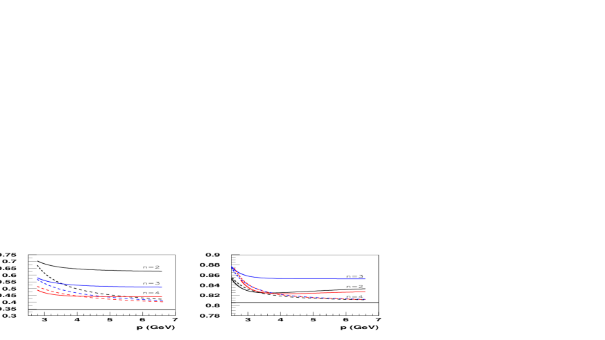
Figure 4: $\frac{\Lambda^{(n)}_{\overline{\text{MS}}}}{\Lambda^{(n)}_{\widetilde{\text{MOMg}}}}$ (left) and $\frac{\Lambda^{(n)}_{\widetilde{\text{MOMc}}}}{\Lambda^{(n)}_{\widetilde{\text{MOMg}}}}$ (right) for $n=2$, $n=3$ and $n=4$. The solid lines are the plots of Eq. (43) with the fitted couplings whereas the dashed lines are the plots with Eq. (44). Horizontal lines are the asymptotic values.

Clearly, the limiting values of these ratios are not the asymptotic values. If we replace in Eq. (43) the coupling $h_{R_{2}}$ by its perturbative expansion with respect to $h_{R_{1}}$

$$h_{R_{2}}=h_{R_{1}}+\sum_{k=1}^{n-1}r_{k}h_{R_{1}}^{k+1}$$ (44)

then the ratios do of course tend towards the asymptotic values $\displaystyle{\exp\left\{\frac{r_{1}}{2\beta_{0}}\right\}}$. The disagreement with respect to the perturbative expansion is not a problem with the lattice data or with the numerical analysis. Indeed the fits do a very good job at extracting a well-behave coupling as illustrated in Fig. 5 which displays the dimensionless scales $a\Lambda^{(4)}_{\overline{\text{MS}}}$, $a\Lambda^{(4)}_{\widetilde{\text{MOMg}}}$ and $a\Lambda^{(4)}_{\widetilde{\text{MOMc}}}$ as a function of the momentum $p$, using Eq. (40) with the fitted couplings at $\beta=6.4$ from the ghost and gluon propagators. $Z_{0}$, the other fitted parameter of Eq. (35), is nearly independent, within a few percent, of the renormalisation scheme as it should in the absence of truncations. It follows that the difficulty to reproduce the asymptotic ratios between the scales of different renormalization schemes, is mainly a consequence of the truncation of the perturbative series of the renormalization constants of the gluon and ghost propagators.

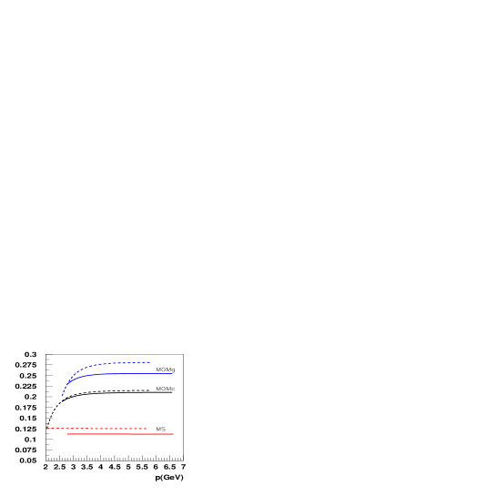
Figure 5: $a\Lambda^{(4)}_{\overline{\text{MS}}}$, $a\Lambda^{(4)}_{\widetilde{\text{MOMg}}}$ and $a\Lambda^{(4)}_{\widetilde{\text{MOMc}}}$ from the gluon propagator (solid lines) and from the ghost propagator (dashed lines) at $\beta$ = 6.4, as a function of the momentum through Eq. (40).

We can substantiate this claim, and estimate the rate of convergence, by the following exercise. We solve $h_{R_{2}}$ in terms of $h_{R_{1}}$ using Eq. (38) at four-loop order

$$\ln\left(\frac{Z_{\Gamma,MOM}}{Z_{0}}\right)=c_{R_{2},0}\ln(h_{R_{2}})+\sum_{k=1}^{3}c_{R_{2},k}h_{R_{2}}^{k}=c_{R_{1},0}\ln(h_{R_{1}})+\sum_{k=1}^{3}c_{R_{1},k}h_{R_{1}}^{k}$$ (45)

Then we plug the solution into Eq. (43). Figure 6 shows the behavior of the corresponding ratios, $\frac{\Lambda^{(4)}_{\overline{\text{MS}}}}{\Lambda^{(4)}_{\widetilde{\text{MOMg}}}}$ and $\frac{\Lambda^{(4)}_{\widetilde{\text{MOMc}}}}{\Lambda^{(4)}_{\widetilde{\text{MOMg}}}}$, as a function of the coupling $h_{\overline{\text{MS}}}$ and $h_{\widetilde{\text{MOMc}}}$ respectively. The effect of the truncation of the perturbative series is manifest for the $\overline{\text{MS}}$ scheme and gives the right order of magnitude of what is actually measured in Tables 5 and 7.

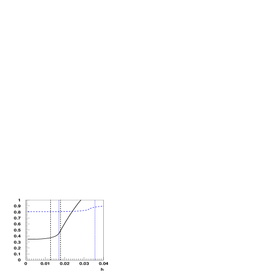
Figure 6: $\frac{\Lambda^{(4)}_{\overline{\text{MS}}}}{\Lambda^{(4)}_{\widetilde{\text{MOMg}}}}$ (solid line) as a function of $h_{\overline{\text{MS}}}$ and $\frac{\Lambda^{(4)}_{\widetilde{\text{MOMc}}}}{\Lambda^{(4)}_{\widetilde{\text{MOMg}}}}$ (dashed line) as a function of $h_{\widetilde{\text{MOMc}}}$. The vertical lines delimit the values spanned by $h_{\overline{\text{MS}}}$ (dashed) and $h_{\widetilde{\text{MOMc}}}$ (dotted) in the fits of the gluon propagator at $\beta=6.4$.

6 Conclusion

We have shown that the lattice formulation of the ghost propagator has the expected perturbative behavior up to four-loop order from 2 GeV to 6 GeV. We have been able to go beyond the qualitative level and to produce quantitative results for the scale $\Lambda_{\overline{\text{MS}}}$ which are pretty consistent with the values extracted from the lattice gluon propagator. We have understood the strong dependence of the effective $\Lambda_{\overline{\text{MS}}}$ scale upon the order of perturbation theory and upon the renormalisation scheme used for the parametrisation of the data. The perturbative series of the $\widetilde{\text{MOM}}$ schemes seem to be asymptotic at three-loop order in the energy range we have probed whereas the $\overline{\text{MS}}$ scheme converges very slowly. If we assume that all perturbative series remain well behaved beyond four-loop above 4 GeV, then we get $\Lambda_{\overline{\text{MS}}}\approx 320$ MeV with a 10% systematic uncertainty. The statistical errors are at the 1% level. This value is also in pretty good agreement with the values of $\Lambda_{\overline{\text{MS}}}$ extracted from the three-gluon vertex in a $\widetilde{\text{MOM}}$ scheme at three-loop order [21], at the same $\beta$’s and with the same lattice sizes. On the other hand it exceeds by 20% the value obtained from the same vertex at $\beta=6.8$ on a $24^{4}$ lattice. This discrepancy motivated the introduction of power corrections which are successful in describing the combined data of the three-gluon vertex [14]. We will show in a forthcoming paper how the power corrections can be unraveled from the lattice propagators alone.

The value quoted above exceeds also by about 30% the previous determinations of the QCD scale in the quenched approximation based on gauge-invariant definitions of the strong coupling constant [22, 23] (take note, for comparison purposes, that our physical unit corresponds to the force parameter $r_{0}$ [24] set approximately to 0.53 fm). However there is also an uncertainty due to the use of the asymptotic one-loop relation between $\Lambda_{\overline{\text{MS}}}$ and the $\Lambda_{\text{L}}$’s. For illustration, let us consider the determination of $\Lambda_{\overline{\text{MS}}}$ using lattice perturbation theory up to three-loop order with the Wilson action [25]. It is possible to estimate the rate of convergence of the ratio $\frac{\Lambda^{(3)}_{\text{L}}}{\Lambda^{(3)}_{\overline{\text{MS}}}}$ as a function of the bare lattice coupling $h_{\text{L}}=\frac{6}{(4\pi)^{2}\beta}$ by inserting the perturbative expansion of $h_{\overline{\text{MS}}}$ into Eq. (43). Figure 7 displays the evolution of this ratio and also of the ratio $\frac{\Lambda^{(3)}_{\square}}{\Lambda^{(3)}_{\overline{\text{MS}}}}$ for the so-called “boosted” lattice scheme which re-express the lattice perturbative series as a function of the coupling $h_{\square}=h_{\text{L}}/\left<plaq\right>$. The mere truncation of the perturbative series introduces an uncertainty on the absolute scale of the lattice schemes which could be as large as 30% in the range of $\beta$ studied in these simulations.

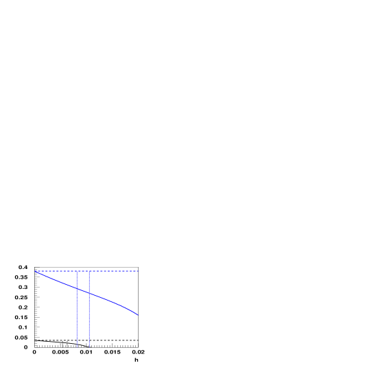
Figure 7: $\frac{\Lambda^{(3)}_{\text{L}}}{\Lambda^{(3)}_{\overline{\text{MS}}}}$ (lower solid line) as a function of $h_{\text{L}}$ and $\frac{\Lambda^{(3)}_{\square}}{\Lambda^{(3)}_{\overline{\text{MS}}}}$ (upper solid line) as a function of $h_{\square}$. The vertical lines (dotted) delimit the values spanned by $h_{\text{L}}$ and $h_{\square}$ in the simulations of [25] $(5.7\leq\beta\leq 6.9)$. The dashed horizontal lines are the asymptotic values.

No strategy can fix the scale $\Lambda_{\text{QCD}}$ to an accuracy better than the uncertainty entailed by the truncation of the perturbative series in the conversion to the $\overline{\text{MS}}$ scheme. We have shown that this error can be larger than the main well-known sources of systematic errors which come from setting the scale $a^{-1}$ and from the continuum extrapolation. If we aim at reducing below 10% the error in the conversion of the $\widetilde{\text{MOM}}$ schemes to the $\overline{\text{MS}}$ scheme, then a look at Figure 6 shows that we need to apply a cut at 6 GeV. Such an analysis would require simulations at $\beta=6.6$ and $\beta=6.8$ on $48^{4}$ and $64^{4}$ lattices respectively, to work at fixed volume and minimize finite-size effects. The existence of several lattice observables, gluon propagator, ghost propagator, three-gluon vertex, from which one can extract independent values of the scale $\Lambda_{\text{QCD}}$, an advantage of the Green function approach, should then allow to disentangle unambiguously the effects of the truncation of the perturbative series from the non-perturbative corrections, and to get a value of $\Lambda_{\overline{\text{MS}}}$ at a true 10% accuracy.

References

• [1] C. Bernard, C. Parrinello and A. Soni, Phys. Rev. D49 (1994) 1585, arXiv:hep-lat/9307001.
• [2] J.E. Mandula, Phys. Rept. 315 (1999) 273, arXiv:hep-lat/9903009.
• [3] D. Becirevic, P. Boucaud, J.P. Leroy, J. Micheli, O. Pène, J. Rodríguez-Quintero, C. Roiesnel, Phys. Rev. D60 (1999) 094509, arXiv:hep-ph/9903364.
• [4] D. Becirevic, P. Boucaud, J.P. Leroy, J. Micheli, O. Pène, J. Rodríguez-Quintero, C. Roiesnel, Phys. Rev. D61 (2000) 114508, arXiv:hep-ph/9910204.
• [5] V.N. Gribov, Nucl. Phys. B139 (1978) 1.
• [6] D. Zwanziger, Nucl. Phys. B412 (1994) 657.
• [7] H. Suman, K. Schilling, Phys. Lett. B373 (1996) 314, arXiv:hep-lat/95120003.
• [8] A. Sternbeck, E.-M. Ilgenfritz, M. Mueller-Preussker, A. Schiller, Nucl. Phys. Proc. Suppl. 140 (2005) 653, arXiv:hep-lat/0409125.
• [9] A. Sternbeck, E.-M. Ilgenfritz, M. Mueller-Preussker, A. Schiller, AIP Conf. Proc. 756 (2005) 284, arXiv:hep-lat/0412011.
• [10] A. Sternbeck, E.-M. Ilgenfritz, M. Mueller-Preussker, A. Schiller, arXiv:hep-lat/0506007.
• [11] S. Furui, H. Nakajima, Phys. Rev. D69 (2004) 074505, arXiv:hep-lat/0305010.
• [12] S. Furui, H. Nakajima, Phys. Rev. D70 (2004) 094504, arXiv:hep-lat/0403021.
• [13] S. Furui, H. Nakajima, arXiv:hep-lat/0503029.
• [14] P. Boucaud & al, JHEP 004 (2000) 006, arXiv:hep-ph/0003020.
• [15] K.G. Chetyrkin, A. Rétey, arXiv:hep-ph/0007088.
• [16] K.G. Chetyrkin, arXiv:hep-ph/0405193.
• [17] T. van Ritbergen, J.A.M. Vermaseren, S.A. Larin, Phys. Lett. B400 (1997) 379, arXiv:hep-ph/9701390.
• [18] G.S. Bali, K. Schilling, Phys. Rev. D47 (1993) 661, arXiv:hep-lat/9208028.
• [19] A. Cucchieri, Nucl. Phys.  B508 (1997) 353, arXiv:hep-lat/9705005.
• [20] T.D. Bakeev & al, Phys. Rev. D69 (2004) 074507, arXiv:hep-lat/0311041.
• [21] P. Boucaud, J.P. Leroy, J. Micheli, O. Pène and C. Roiesnel, JHEP10 (1998) 017, arXiv:hep-ph/9810322.
• [22] S. Capitani, M. Lüscher, R. Sommer and H. Wittig, Nucl. Phys. B544 (1999) 669, arXiv:hep-lat/9810063.
• [23] S. Booth & al, Phys. Lett. 519 (2001) 229, arXiv:hep-lat/0103023.
• [24] S. Necco and R. Sommer, Nucl. Phys. B622 (2002) 328, arXiv:hep-ph/0109093.
• [25] M. Göckeler & al, arXiv:hep-lat/0502212.