SHEP-0516

A Numerical Study of Partially Twisted Boundary Conditions
J.M. Flynn, A. Jüttner and C.T. Sachrajda
(UKQCD Collaboration)
School of Physics and Astronomy, University of Southampton,
Southampton, SO17 1BJ, UK.

Abstract
We investigate the use of partially twisted boundary conditions in a lattice simulation with two degenerate flavours of improved Wilson sea quarks. The use of twisted boundary conditions on a cubic volume ($L^{3}$) gives access to components of hadronic momenta other than integer multiples of $\mathchoice{{2\pi\over L}}{2\pi/L}{2\pi/L}{2\pi/L}$. Partial twisting avoids the need for new gluon configurations for every choice of momentum, while, as recently demonstrated, keeping the finite-volume errors exponentially small for the physical quantities investigated in this letter. In this study we focus on the spectrum of pseudo scalar and vector mesons, on their leptonic decay constants and on $Z_{P}$, the matrix element of the pseudo scalar density between the pseudo scalar meson and the vacuum. The results confirm the momentum shift imposed by these boundary conditions and in addition demonstrate that they do not introduce any appreciable noise. We therefore advocate the use of partially twisted boundary conditions in applications where good momentum resolution is necessary.

           PACS: 11.15 Ha, 12.38 Gc

1 Introduction

In lattice simulations of QCD on a cubic volume ($V=L^{3}$) with periodic boundary conditions on the fields, the components of hadronic momenta $p_{i}$ are quantized in integer multiples of $\mathchoice{{2\pi\over L}}{2\pi/L}{2\pi/L}{2\pi/L}$. For currently available lattices this implies that the lowest non-zero momentum is large, typically $500\,\mathrm{MeV}$ or so, and there are large gaps between neighbouring momenta. This limits the phenomenological reach of simulations, particularly for momentum dependent quantities such as the form-factors of weak semileptonic decays of hadrons. In ref. [1] Bedaque proposed the use of twisted boundary conditions for the quark fields $\psi$

$$\psi(x_{i}+L)=e^{i\theta_{i}}\,\psi(x_{i})\,.$$ (1)

Twisted boundary conditions allow for simulations with arbitrary components of hadronic momenta. For example, the momentum of a meson composed of a quark with flavour $1$ satisfying boundary conditions with a twisting angle $\vec{\theta}_{1}=(\theta_{11},\theta_{12},\theta_{13})$ and an antiquark of flavour $2$ with angle $\vec{\theta}_{2}$  is

$$\vec{p}=\mathchoice{{2\pi\over L}}{2\pi/L}{2\pi/L}{2\pi/L}\,\vec{n}-\frac{\vec{\theta}_{1}-\vec{\theta}_{2}}{L}\,,$$ (2)

where $\vec{n}$ is a vector of integers.

The practical difficulty in using twisted boundary conditions in lattice simulations with dynamical quarks is that it requires the generation of a new set of gauge field configurations for every choice of twisting angle(s). In refs. [3, 4] it was shown that for many physical quantities one can use partially twisted boundary conditions, i.e. impose twisted boundary conditions for the valence quarks but periodic boundary conditions for the sea quarks, thus eliminating the need for new simulations for every choice of momentum and making the technique practicable. The physical quantities for which partially twisted boundary conditions can be applied include those with at most a single hadron in the initial and final states (and possibly even in intermediate states), for which the finite-volume effects decrease exponentially with the volume. For these processes the finite-volume effects depend on the twisting angle(s) but remain exponentially small.

For some processes with energies above a two-body threshold, such as $K\to\pi\pi$ decays with the two-pions in an isospin zero state, the finite-volume effects decrease only as powers of the volume and must be subtracted for acceptable precision to be reached. We are not able to perform these subtractions if partially twisted boundary conditions are used. Here we will only consider processes for which such a problem does not arise.

In this letter we confirm the theoretical results of ref. [3] in a numerical study of partially twisted boundary conditions for dynamical, non-perturbatively improved Wilson fermions. In particular we find that:

• The energies of $\pi$ and $\rho$-mesons (with masses below the two-pion threshold) satisfy the expected dispersion relation

  $$E_{\pi,\,\rho}^{2}=m_{\pi,\,\rho}^{2}+\left(\vec{p}_{\rm lat}-{\vec{\theta}_{1}-\vec{\theta}_{2}\over L}\right)^{2},$$ (3)

  where $\vec{\theta}_{1}$ and $\vec{\theta}_{2}$ are the twisting angles of the two valence quarks and $\vec{p}_{\mathrm{lat}}=(\mathchoice{{2\pi\over L}}{2\pi/L}{2\pi/L}{2\pi/L})\vec{n}$ is the contribution to the meson’s momentum introduced by the Fourier transform of the correlation function.

  This study extends the one in ref. [2] where the dispersion relation for pseudo scalar mesons with twisted boundary conditions in the quenched approximation was found to be consistent with expectations.

• The values of the leptonic decay constants of $\pi$ and $\rho$ mesons and of the matrix element $\langle 0|P|\pi\rangle$ of the pseudo scalar density $P$ are independent of the twisting angles as expected.

A further reassuring result of our study is that twisted boundary conditions do not introduce additional noise in the data. As we increase the meson’s momentum by suitably varying the angles $\vec{\theta}_{1,2}$, the statistical errors on meson masses and matrix elements increase smoothly. However, when comparing results obtained with twisted and periodic boundary conditions with similar momenta (i.e. momenta close to $\mathchoice{{2\pi\over L}}{2\pi/L}{2\pi/L}{2\pi/L}$ or $\sqrt{2}(\mathchoice{{2\pi\over L}}{2\pi/L}{2\pi/L}{2\pi/L})$) the errors are found to be comparable.

The plan of the remainder of this letter is as follows. In the next section we present the details of our computation, the parameters of the simulation (including the choice of twisting angles) and a description of the analysis. We present our results in sec. 3 and conclusions in sec. 4.

2 Details of the Simulation and Analysis

We study meson observables on sets of gauge configurations which were generated with two degenerate flavours of sea quarks using non-perturbatively improved Wilson fermions and the plaquette gauge action on the torus with periodic boundary conditions ($\beta=5.2$, $a\approx 0.1\,\mathrm{fm}$, $c_{\rm SW}=2.0171$, $(L/a)^{3}\times T/a=16^{3}\times 32$). We used the ensembles of field configurations which were studied in detail in [5, 6] and took over the suggested separation of measurements by $40$ trajectories in our analysis. The simulated quark masses are summarized in table 1. Propagators and correlators were calculated using the FermiQCD libraries [7, 8, 9]. We stress that the aim of the present study is to investigate the consistency and effectiveness of using partially twisted boundary conditions at fixed values of the quark mass. We do not attempt to perform a chiral extrapolation.

$\kappa_{\mathrm{val}}=\kappa_{\mathrm{sea}}$	$m_{\pi}/m_{\rho}$	$N_{\mathrm{meas}}$
0.13500	0.697(11)	200
0.13550	0.566(16)	200

Table 1: Simulation parameters.

For each flavour of valence quark we impose the boundary conditions in eq. (1) for a variety of twisting angles $\vec{\theta}=(\theta_{1},\theta_{2},\theta_{3})$. When evaluating the corresponding propagators we make use of the change of quark field variables

$$\psi(x)=e^{i{\vec{\theta}\cdot\vec{x}\over L}}\tilde{\psi}(x),$$ (4)

where $\tilde{\psi}(x)$ satisfies periodic boundary conditions. The phase factor cancels in all terms of the lattice fermion action except for the spatial hopping terms which now become (for $i=1,2,3$)

$$\overline{\tilde{\psi}}(x)\left[e^{i{a\theta_{i}\over L}}U_{i}(x)(1-\gamma_{i})\tilde{\psi}(x+\hat{i})+e^{-i{a\theta_{i}\over L}}U^{\dagger}_{i}(x-\hat{i})(1+\gamma_{i})\tilde{\psi}(x-\hat{i})\right].$$ (5)

In practice therefore, the partially twisted quark propagator can be computed by inverting the standard improved Wilson-Dirac operator in a gauge field background where the link variables {$U_{i}(x)$} have been replaced by {$e^{i{a\theta_{i}\over L}}U_{i}(x)$}.

The physical observables which we study in this letter are the energies and leptonic decay constants of the pseudo scalar and vector mesons and the matrix element of the pseudo scalar density. In order to determine these, we compute the following correlation functions:

$$C_{A_{0}P}(t,\vec{p}) = \sum\limits_{\vec{x}}e^{i\vec{p}_{\mathrm{lat}}\cdot\,\vec{x}}\langle 0|A^{I}_{0}(\vec{x},t)P^{\dagger}(0)|0\rangle\,,$$ (6)

$$C_{PP}(t,\vec{p}) = \sum\limits_{\vec{x}}e^{i\vec{p}_{\mathrm{lat}}\cdot\,\vec{x}}\langle 0|P(\vec{x},t)P^{\dagger}(0)|0\rangle\,,$$ (7)

$$C_{A_{0}A_{0}}(t,\vec{p}) = \sum\limits_{\vec{x}}e^{i\vec{p}_{\mathrm{lat}}\cdot\,\vec{x}}\langle 0|A_{0}^{I}(\vec{x},t)(A_{0}^{I}(0))^{\dagger}|0\rangle\,,$$ (8)

$$C_{V_{i}V_{i}}(t,\vec{p}) = \sum\limits_{\vec{x}}e^{i\vec{p}_{\mathrm{lat}}\cdot\,\vec{x}}\langle 0|V_{i}^{I}(\vec{x},t)(V_{i}^{I}(0))^{\dagger}|0\rangle\quad\mbox{(no sum on $i$)}\,,$$ (9)

where $P(x)$ is the pseudo scalar density

$$P(x)=\overline{\psi}_{2}(x)\gamma_{5}\psi_{1}(x)$$ (10)

for quarks of flavour $1$ and $2$ (with twisting angles $\vec{\theta}_{1}$ and $\vec{\theta}_{2}$), and $V^{I}_{\mu}(x)$ and $A^{I}_{\mu}(x)$ are the improved vector and axial-vector currents

$$V^{I}_{\mu}(x) = \overline{\psi}_{2}(x)\gamma_{\mu}\psi_{1}(x)+ac_{V}(g_{0})\,{1\over 2}(\partial^{\ast}_{\nu}+\partial_{\nu})\overline{\psi}_{2}(x)\sigma_{\mu\nu}\psi_{1}(x)$$

$$A^{I}_{\mu}(x) = \overline{\psi}_{2}(x)\gamma_{\mu}\gamma_{5}\psi_{1}(x)+ac_{A}(g_{0}){1\over 2}(\partial^{\ast}_{\mu}+\partial_{\mu})P(x)\,.$$

Here, $\partial_{\mu}$ and $\partial^{\ast}_{\mu}$ are the forward and backward derivatives and $c_{V}(g_{0})$ and $c_{A}(g_{0})$ are improvement coefficients which we take from [10] and [11] respectively. Since we are primarily interested in the effects of twisted boundary conditions we do not attempt to compute the renormalization constants of $P$, $V_{\mu}$ and $A_{\mu}$, nor do we implement improvement factors of the form $1+b(g_{0})m_{q}a$, where $m_{q}$ is the mass of the quark. The inclusion of these factors would of course be necessary if we were attempting to determine the physical leptonic decay constants. However, they are overall factors for each choice of quark mass and are independent of the twisting angles, while it is precisely the dependence on these angles which is the object of our study.

The momentum, $\vec{p}$, of the meson is given by

$$\vec{p}=\vec{p}_{\mathrm{lat}}-{\vec{\theta}_{1}-\vec{\theta}_{2}\over L}\,,$$ (11)

where $p_{\mathrm{lat}}=(\mathchoice{{2\pi\over L}}{2\pi/L}{2\pi/L}{2\pi/L})\vec{n}$ and $\vec{n}$ is a vector of integers.

At large values of $t$ the time dependences of (6)–(9) approach:

$$C_{A_{0}P}(t,\vec{p}\,) \to {1\over E_{\pi}}\,Z_{P}\,M_{0}(\vec{p}\,)\,e^{-E_{\pi}\,T/2}\sinh((t-T/2)E_{\pi}),$$ (12)

$$C_{PP}(t,\vec{p}\,) \to {1\over E_{\pi}}\,Z_{P}^{2}\,e^{-E_{\pi}\,T/2}\cosh((t-T/2)E_{\pi}),$$ (13)

$$C_{A_{0}A_{0}}(t,\vec{p}\,) \to {1\over E_{\pi}}\,M_{0}^{2}(\vec{p}\,)\,e^{-E_{\pi}\,T/2}\cosh((t-T/2)E_{\pi}),$$ (14)

$$C_{V_{i}V_{i}}(t,\vec{p}\,) \to {1\over E_{\rho}}\,N^{2}_{i}(\vec{p}\,)\,e^{-E_{\rho}\,T/2}\cosh((t-T/2)E_{\rho})\;\quad(i=1,2,3),$$ (15)

where, for each choice of quark masses, we have denoted the lightest pseudo scalar and vector mesons by $\pi$ and $\rho$ respectively and $E_{\pi}$ and $E_{\rho}$ are the corresponding energies which we expect to satisfy the dispersion relations in eq. (3). The notation for the matrix elements is as follows:

$$Z_{P} = \langle 0|P(0)|\pi(\vec{p}\,)\rangle,$$ (16)

$$M_{0}(\vec{p}\,) = \langle 0\,|\,A_{0}(0)\,|\,\pi(\vec{p}\,)\rangle=f_{\pi}E_{\pi},$$ (17)

$$N^{2}_{i}(\vec{p}\,) = \sum_{\lambda}|\langle\,0|\,V_{i}(0)\,|\,\rho(\vec{p},\lambda)\rangle|^{2}=f_{\rho}^{2}m_{\rho}^{2}\left(1+{p_{i}^{2}\over m_{\rho}^{2}}\right)\,$$ (18)

where the index $\lambda$ labels the $\rho$-meson’s polarization state.

In this letter we study the validity of the dispersion relation in eq. (3) and the independence of $f_{\pi}$, $f_{\rho}$ and $Z_{P}$ of the momentum. We evaluate the quark propagators for four values of the twisting angle $\vec{\theta}$:

$$\vec{\theta}=\vec{0},\ (2,0,0),\ (0,\pi,0)\ \textrm{and}\ (3,3,3)\,.$$ (19)

For each value of $\kappa_{\mathrm{val}}$, quark and antiquark propagators with all possible pairs $\vec{\theta}_{1}$ and $\vec{\theta}_{2}$ were combined to construct correlation functions for mesons with a variety of momenta. Moreover we also combined them with Fourier momenta $\vec{p}_{\mathrm{lat}}=(0,\pm\,\mathchoice{{2\pi\over L}}{2\pi/L}{2\pi/L}{2\pi/L},0)$ to increase the range of momenta which can be reached. When presenting our results in the following section, we include for comparison results without twisting ($\vec{\theta}_{1}=\vec{\theta}_{2}=0$), obtained by averaging over the $12$ equivalent momenta with $|\vec{p}_{\mathrm{lat}}|=\sqrt{2}\times\mathchoice{{2\pi\over L}}{2\pi/L}{2\pi/L}{2\pi/L}$ and those obtained by averaging over the eight equivalent momenta with $|\vec{p}_{\mathrm{lat}}|=\sqrt{3}\times\mathchoice{{2\pi\over L}}{2\pi/L}{2\pi/L}{2\pi/L}$. Of course this averaging reduces the statistical errors and this should be borne in mind when comparing the errors at these untwisted momenta with those at momenta with $\vec{\theta}_{1}-\vec{\theta}_{2}\neq\vec{0}$ for which such averaging is not possible.

Applying the jackknife procedure to the data for the correlation functions in eqs. (6)–(8), we have extracted all observables in the pseudo scalar channel from a combined non-linear $\chi^{2}$ fit to the functional form suggested by (12)–(14), (16) and (17). The fit-ranges were chosen to yield compatible results under variation of the range by at least one unit in $t/a$. We applied the same procedure in the vector channel, combining the data for the correlation function (9) for $i=1,2$ and $3$ in one fit using the expressions in eqs. (15) and (18).

3 Results

The series of plots in figures 1 and 3 show our data as a function of $(\vec{p}L)^{2}$ in the range $|\vec{p}L|\in[0,\sqrt{3}\times 2\pi]$. Fig. 1 contains the results for the energies as a function of momentum and fig. 3 those for the decay constants and $Z_{P}$. To ease orientation, the positions of the discrete Fourier momenta $|\vec{p}_{\rm lat}L|=0$, $2\pi$, $\sqrt{2}\times 2\pi$ and $\sqrt{3}\times 2\pi$ are indicated by dashed vertical lines. We emphasize that it is only at these values of momenta that one can obtain results using periodic boundary conditions. In fig. 2 we zoom into the region $|\vec{p}\,L|\leq 2\pi$ for the dispersion relations. In this region we would expect lattice artefacts to be small and the use of twisted boundary conditions to be particularly useful.

In each plot, the (blue) triangles correspond to points in which the correlation function was evaluated with $\vec{p}_{\mathrm{lat}}=\vec{0}$, but with all possible pairs of $\vec{\theta}_{1}$ and $\vec{\theta}_{2}$ from the set in (19). The (red) diamonds and (green) squares represent the results obtained with $\vec{p}_{\mathrm{lat}}=(0,2\pi/L,0)$ and $\vec{p}_{\mathrm{lat}}=-(0,2\pi/L,0)$ respectively, combined with all possible pairs of $\vec{\theta}_{1}$ and $\vec{\theta}_{2}$. The four points with $\vec{\theta}_{1}=\vec{\theta}_{2}=\vec{0}$ with $|\vec{p}_{\mathrm{lat}}|=0,\ 2\pi/L,\ \sqrt{2}\times 2\pi/L$ and $\sqrt{3}\times 2\pi/L$ are denoted by (black) circles.

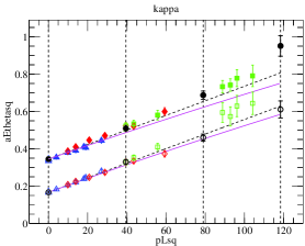
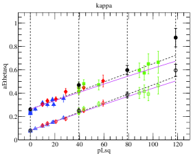
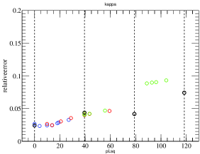
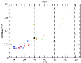
Figure 1: The plots in the first line illustrate the results for the dispersion relation for the $\pi$ and the $\rho$ (empty and full symbols respectively) for the two choices of the quark mass. In the second line we show the corresponding relative error as a function of the momentum.

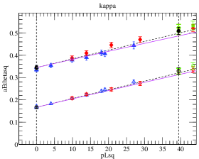
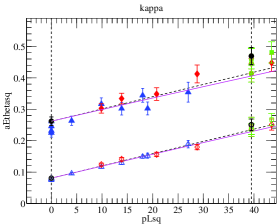
Figure 2: Magnified view of the dispersion relation of fig. 1 in the interval $|\vec{p}_{\rm lat}|\in[0,2\pi]$.

	$\kappa=0.13500$		$\kappa=0.13550$
	$\pi$	$\rho$	$\pi$	$\rho$
$\chi^{2}/\mathrm{d.o.f}|_{\mathrm{(\ref{expecteddisprel2})}}$	0.3	1.0	0.6	1.7
$\chi^{2}/\mathrm{d.o.f}|_{\mathrm{(\ref{expecteddisprel1})}}$	1.8	2.5	0.9	2.1
$\Delta^{2}$ from (20)	0.0040(1)	0.0042(2)	0.0040(1)	0.0048(4)

Table 2: $\chi^{2}$/d.o.f. for the lattice data with respect the expectations eqs. (20) and (21) with $\Delta^{2}=a^{2}/L^{2}=0.0039$ (first two rows) and the results obtained from a fit to (20) with $\Delta^{2}$ left as a parameter of the fit (third row).

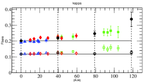
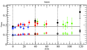
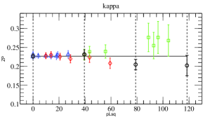
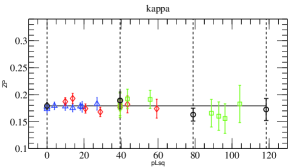
Figure 3: The first line shows the results for the $\pi$ and $\rho$ decay constant (empty and full symbols respectively) and the second line shows the matrix element (16) for the two choices of the quark mass. In each plot the horizontal lines represent the central value at $\vec{p}_{\mathrm{lat}}=\vec{\theta}_{1}=\vec{\theta}_{2}=0$.

For the discussion of our results it is convenient to rewrite the dispersion relation in eq. (3) in the form

$$(aE_{\pi/\rho})^{2}=(am_{\pi/\rho})^{2}+\Delta^{2}(\vec{p}\,L)^{2}$$ (20)

where $\Delta^{2}=(a/L)^{2}=0.0039$. The dispersion relation (20) is displayed as the dashed line in the plots of fig. 1. In the first row of table 2 we present the $\chi^{2}/$d.o.f of the comparison of our data to eq. (20) over the range $0\leq|\vec{p}\,|^{2}L^{2}\leq(2\pi)^{2}$ using the values of the meson masses obtained from fits at zero momenta. In the third row of the table we present the values of $\Delta^{2}$ obtained by fitting the lattice data to the functional form in eq. (20) over the same range in momentum, but allowing $\Delta^{2}$ to be a parameter of the fit. We note that our values for the ratios $m_{\pi}/m_{\rho}$ agree with those found earlier on the same configurations in [5].

As the momentum of the meson grows so do the expected discretization effects in the dispersion relation. For example, a free scalar particle with a wave-function $\phi(x)$ satisfying the (Minkowski-Space) Klein-Gordon equation $(\square+m^{2})\phi(x)=0$, with a generic discretized second derivative defined by $\partial^{2}f(x)/\partial x^{2}=(f(x+a)+f(x-a)-2f(x))/a^{2}$, satisfies the following lattice dispersion relation:

$$\sinh^{2}\bigg{(}{aE_{\pi/\rho}\over 2}\bigg{)}=\sinh^{2}\bigg{(}{am\over 2}\bigg{)}+\sum_{i}\sin^{2}\bigg{(}\Delta{p_{i}L\over 2}\bigg{)}.$$ (21)

To indicate the possible size of lattice artefacts we plot the dispersion relation of eq. (21) as the solid curve in fig. 1. We stress, however, that in an interacting theory the discretization errors will in general be different from those in eq. (21). Indeed there seems to be no evidence from our data that eq. (21) is a particularly good representation of the lattice artefacts (see the second row of table 2, where we show the $\chi^{2}/$d.o.f. from a comparison of our data with (21)). At small momenta the solid curve merges of course with the dashed line representing the continuum dispersion relation.

We conclude from the results for the dispersion relation plotted in figs. 1 and 2 that the use of partially twisted boundary conditions is beautifully consistent with expectations, particularly at low momenta where the lattice artefacts are small. An important further observation is that there is no evidence in our data that the introduction of twisted boundary conditions increases significantly the statistical or systematic uncertainties. This is illustrated in the second line of figure 1, which shows the relative error in the pion energy

$$\delta_{E_{\pi}}\equiv{\delta E_{\pi}\over E_{\pi}}$$ (22)

as $|\vec{p}\,L|$ is varied. The error $\delta E_{\pi}$ is the jackknife error, including the statistical error and the systematic uncertainty stemming from the improvement constants in the improved quark currents. The plot shows that the errors increase smoothly as the momentum increases, and that no appreciable additional noise is introduced by partial twisting . We observe the same behaviour for all analyzed quantities.

In fig. 3 we plot our results for the decay constants $f_{\pi}$ and $f_{\rho}$ and for $Z_{P}$. The values for $af_{\pi}$ agree with the ones obtained in [6] at $|\vec{p}\,L|=0$. Again we see that the results are completely consistent with theoretical expectations, being independent of the twisting angles and Fourier momenta.

4 Conclusions

We have investigated the use of partially twisted boundary conditions in evaluating the energies of pseudo scalar and vector mesons and their leptonic decay constants. The results are very encouraging; it does appear that the method allows the evaluation of physical quantities with any momentum. Moreover the use of these boundary conditions does not appear to increase the errors in any appreciable way. It will be important to monitor whether this continues to be true as the quark masses are decreased. Once the quark masses are such that two-pion intermediate states contribute significantly to the $\rho$-meson’s correlation function the finite-volume effects will no longer fall exponentially with the volume, but only as powers. For the pion observables studied in this paper this is not the case.

Partially twisted boundary conditions will be particularly useful for evaluating momentum-dependent physical quantities. One important application is to the determination of the form-factors of semileptonic weak decays of heavy ($D$ and $B$) mesons to light mesons. For these processes, with conventional periodic boundary conditions, the initial and final state hadrons are restricted to have momenta $(\mathchoice{{2\pi\over L}}{2\pi/L}{2\pi/L}{2\pi/L})\vec{n}$ where $\vec{n}$ is a vector of integers. In order to avoid lattice artefacts the possible values of $|\vec{n}|$ are frequently limited to $0$, $1$, and perhaps $\sqrt{2}$. Thus, for any particular choice of quark masses, the number of values of the momentum transfer, $q^{2}$, or the light meson energy, $E$, is also very limited. Moreover, chiral extrapolations are conveniently performed at fixed $q^{2}$ [13, 14, 15] or fixed $E$ [16, 17, 18, 19] (and heavy quark extrapolations at fixed $E$), but $q^{2}$ and $E$ vary with both the momentum and quark masses. Ansätze for the form factors, such as the Becirevic-Kaidalov [20] model, are used to interpolate and extrapolate simulation data to sets of common $q^{2}$ or $E$ values before the extrapolations are performed. Using twisted boundary conditions would enable the form factors to be evaluated directly at these common values, removing the need for the intermediate form-factor fit.

For some other physical quantities, such as the moments of hadronic deep inelastic structure functions or light-cone distribution amplitudes, it may be helpful to use twisted boundary conditions even though it is not strictly necessary. The corresponding matrix elements are proportional to factors of $p_{i}$, where $\vec{p}$ is the momentum of the hadron, so that the correlation functions must be computed with $\vec{p}\neq 0$. The use of twisted boundary conditions allows $|\vec{p}\,|$ to be decreased and hence the lattice artefacts to be reduced. Moreover by varying $\vec{p}$ one can verify that the leading twist component has been extracted correctly.

Following the successful conclusion of this exploratory numerical study of the implementation of partially twisted boundary conditions we now look forward to applying them in lattice computations of a wide variety of phenomenologically important quantities.

Acknowledgements We warmly thank Daragh Byrne, Steve Downing and Craig McNeile for their support with QCDgrid and Massimo di Pierro for help using FermiQCD. We thank the Iridis parallel computing team at the University of Southampton, in particular Oz Parchment and Ivan Wolton, for their assistance. We also acknowledge Alan Irving, Craig McNeile and Chris Michael for correspondence on the gauge field configurations. This work was supported by PPARC grants PPA/G/S/2002/00467 and PPA/G/O/2002/00468.

References

- [1] P.F. Bedaque, Phys. Lett. B593 (2004) 82, nucl-th/0402051.
- [2] G.M. de Divitiis, R. Petronzio and N. Tantalo, Phys. Lett. B595 (2004) 408, hep-lat/0405002.
- [3] C.T. Sachrajda and G. Villadoro, Phys. Lett. B609 (2005) 73, hep-lat/0411033.
- [4] P.F. Bedaque and J.W. Chen (2004), hep-lat/0412023.
- [5] UKQCD Collaboration, C.R. Allton et al., Phys. Rev. D65 (2002) 054502, hep-lat/0107021.
- [6] UKQCD Collaboration, C.R. Allton et al., Phys. Rev. D70 (2004) 014501, hep-lat/0403007.
- [7] M. Di Pierro, Comput. Phys. Commun. 141 (2001) 98, hep-lat/0004007.
- [8] M. Di Pierro, Nucl. Phys. Proc. Suppl. 106 (2002) 1034, hep-lat/0110116.
- [9] FermiQCD Colaboration Collaboration, M. Di Pierro et al., Nucl. Phys. Proc. Suppl. 129 (2004) 832, hep-lat/0311027.
- [10] J. Harada, S. Hashimoto, A.S. Kronfeld and T. Onogi, Phys. Rev. D67 (2003) 014503, hep-lat/0208004.
- [11] M. Della Morte, R. Hoffmann and R. Sommer, JHEP 03 (2005) 029, hep-lat/0503003.
- [12] A. Irving, C. McNeile and C. Michael, private communications.
- [13] UKQCD Collaboration, K.C. Bowler et al., Phys. Lett. B486 (2000) 111, hep-lat/9911011.
- [14] A. Abada et al., Nucl. Phys. B619 (2001) 565, hep-lat/0011065.
- [15] UKQCD Collaboration, K.C. Bowler, J.F. Gill, C.M. Maynard and J.M. Flynn, JHEP 05 (2004) 035, hep-lat/0402023.
- [16] JLQCD Collaboration, S. Aoki et al., Phys. Rev. D64 (2001) 114505, hep-lat/0106024.
- [17] Fermilab Lattice Collaboration, C. Aubin et al., Phys. Rev. Lett. 94 (2005) 011601, hep-ph/0408306.
- [18] J. Shigemitsu et al., Nucl. Phys. Proc. Suppl. 140 (2005) 464, hep-lat/0408019.
- [19] M. Okamoto et al., Nucl. Phys. Proc. Suppl. 140 (2005) 461, hep-lat/0409116.
- [20] D. Becirevic and A.B. Kaidalov, Phys. Lett. B478 (2000) 417, hep-ph/9904490.