Lattice QCD equation of state : improving the differential method

Abstract

We propose an improvement of the differential method for the computation of the equation of state of QCD from lattice simulations. In contrast to the earlier differential method our technique yields positive pressure for all temperatures including in the transition region. Employing it on temporal lattices of 8, 10 and 12 sites and by extrapolating to zero lattice spacing we obtained the pressure, energy density, entropy density, specific heat and speed of sound in quenched QCD for $0.9\leq T/T_{c}\leq 3$. A comparison of our results is made with those from the dimensional reduction approach and a conformal symmetric theory at high-temperature.

1. Introduction

There is growing acceptance of the view that in the ongoing experiments in Relativistic Heavy Ion Collider (RHIC) at Brookhaven a new form of matter has been created  [?]. This new form of matter is thought to be a fluid of strongly interacting quarks and gluons. In lattice studies of quenched QCD it was found earlier that the entropy density $s$  [?,?] and the mean free time $\tau$, derived from the electrical conductivity  [?], together gave rise to a dimensionless number $\tau s^{1/3}\approx 0.8$  [?]. In the non-relativistic limit this dimensionless number measures the mean free path in units of interparticle spacing, and is therefore large in a gas but of order unity in a liquid. This indicated that the deviation of the energy density ($\epsilon$) and pressure ($P$) in the high temperature phase of QCD from their ideal gas values may be due to a previously underappreciated feature of the plasma phase— that it is far from being a weakly interacting gas.

Earlier expectations that a weakly interacting gas of quarks and gluons would be formed in the experiments were based on perturbative calculations  [?] which failed to reproduce these lattice results  [?]. There have been many suggestions for the physics implied by the lattice data— the inclusion of various quasi-particles  [?], the necessity of large resummations  [?], and effective models  [?] being a few. Investigation of screening masses also gave evidence for strong departure from perturbative results  [?,?,?,?,?]. Interestingly, there has been a suggestion that conformal field theory comes closer to the lattice result  [?]. This assumes more significance in view of the fact that a bound on the ratio of the shear viscosity and the entropy density, $s$, conjectured from the AdS/CFT correspondence  [?] lies close to that inferred from analysis of RHIC data  [?] and its direct lattice measurement  [?,?] as well as the lattice results of a different transport coefficient  [?].

The equation of state (EOS) is one of the most basic inputs into the analysis of experimental data. Two decades ago, a method was devised to compute the EOS of QCD on the lattice [?]. However, soon it was found  [?] that this method yielded negative $P$ near the critical temperature, $T_{c}$. At that time it was thought that this problem of the “differential method”, as it is called now, is solely due to the use of perturbative formulae for various derivatives of the coupling. To cure this problem of negative pressure the non-perturbative “integral method” was introduced  [?,?]. It bypasses the use of perturbative couplings by employing the thermodynamic relation $F=-PV$ and using a non-perturbative but phenomenologically fitted QCD $\beta$-function. If the EOS were to be evaluated by the integral method then fluctuation measures (e.g. the specific heat at constant volume $C_{\scriptscriptstyle V}$) can only be evaluated through numerical differentiation, which is prone to large errors  [?]. Moreover, the relation $F=-PV$ assumes the system to be homogeneous. Since the pure gauge phase transition in QCD is of first order the system is not homogeneous at $T_{c}$. Thus one makes an unknown systematic error in the integral method computation by integrating through $T_{c}$. This is in addition to a small systematic error due to setting $P=0$ just below $T_{c}$ and the numerical integration errors. Clearly, our confidence in the lattice results on the EOS would be boosted if an entirely different method of EOS determination yields the same results: it would tantamount to a good control over many systematic errors in both.

In this paper we propose a modification of the differential method which gives positive pressure over the entire temperature range for even relatively coarser lattices . We choose the temporal lattice spacing ($a_{\tau}$) to set the scale of the theory, in contrast to the choice of the spatial lattice spacing ($a_{s}$) in the approach of  [?]. This change of scale is analogous to the use of different renormalization schemes. As a consequence, our method could be called the t-favoured scheme and the method of Ref.  [?] may be called the s-favoured scheme. In fact, in a different context, this choice of scale has already been used in Ref.  [?]. Here we show that this choice leads to positive pressure for the entire temperature range, even when one uses one-loop order perturbative couplings. Since the operator expressions are derived with an asymmetry between the two lattice spacings $a_{s}$ and $a_{\tau}$, the s-favoured and t-favoured schemes give different expressions for the pressure. In that sense the use of t-favoured scheme is tantamount to the use of better operators.

Being a differential method the t-favoured scheme can be easily extended for the calculation of fluctuation measures like $C_{\scriptscriptstyle V}$, following the formalism developed in Ref.  [?]. In a theory with only gluons there is only this one fluctuation measure. Related to this is a kinetic variable, the speed of sound, $C_{s}$, which can also be evaluated in any operator method. We report measurements of both in the temperature range $0.9T_{c}\leq T\leq 3T_{c}$ through a continuum extrapolation of results obtained using successively finer lattices.

Not only do these quantities provide further tests of all the models which try to explain the lattice data on the EOS they also have direct physical relevance to experiments at RHIC. In a canonical ensemble the specific heat at constant volume is a measure of energy fluctuations. It was suggested in Ref.  [?] that event-by-event temperature fluctuation in the heavy-ion collision experiments can be used to measure $C_{\scriptscriptstyle V}$. The speed of sound, on the other hand, controls the expansion rate of the fire-ball produced in the heavy-ion collisions. Thus the value of $C_{s}$ is an important parameter in the hydrodynamic studies. It has been noted that the magnitude of elliptic flow in heavy-ion collisions is sensitive to the value of $C_{s}$  [?].

The measurement of $C_{\scriptscriptstyle V}$ and $C_{s}$ also directly test the relevance of conformal symmetry to finite temperature QCD. QCD is known to generate the scale, $\Lambda_{QCD}$, dynamically and thus break conformal invariance. The strength of the breaking of this symmetry at any scale is parametrized by the $\beta$-function. An effective theory which reproduces the results of thermal QCD at long-distance scales could still be close to a conformal theory. The result of Ref.  [?] for the entropy density, $s$, in a Yang-Mills theory with four supersymmetry charges (${\cal N}=4$ SYM) and large number of colours, $N_{c}$, at strong coupling, is

$$\frac{s}{s_{0}} = f(g^{2}N_{c}),\quad{\rm where}\quad s_{0}=\frac{2}{3}\pi^{2}N_{c}^{2}T^{3}\quad{\rm and}\quad$$ (1)

$$f(x) = \frac{3}{4}+\frac{45}{32}\zeta(3)x^{-3/2}+\cdots,$$ (2)

$g$ being the Yang-Mills coupling . For our case of $N_{c}=3$, the well-known result for the ideal gas, $s_{0}=4(N_{c}^{2}-1)\pi^{2}T^{3}/45$ takes into account, through the factor $N_{c}^{2}-1$, the relatively important difference between a $SU(N_{c})$ and an $U(N_{c})$ theory.

The paper is organized as follows. In the next section we present the formalism and lead up to the measurement of $C_{\scriptscriptstyle V}$ and $C_{s}^{2}$ on the lattice in Section 2.2. In Section 3 we give details of our simulations and our results. Finally, in Section 4 we present a discussion of the results.

2. Formalism

Various derivatives of the partition function, ${\cal Z}(V,T)$, where $V$ is the volume and $T$ the temperature, lead to thermodynamic quantities of interest. In particular the energy density, $\epsilon$, and the pressure, $P$, are given by the first derivatives of $\ln{\cal Z}$,

$$\epsilon=\left(\frac{T}{V}\right)\left.T\frac{\partial\ln{\cal Z}(V,T)}{\partial T}\right|_{V}\qquad{\rm and}\qquad P=\left(\frac{T}{V}\right)\left.V\frac{\partial\ln{\cal Z}(V,T)}{\partial V}\right|_{T}.$$ (3)

The second derivatives are measures of fluctuations. In the absence of chemical potentials a change of volume of a relativistic gas alters its pressure by changing particle numbers. As a result there is only one second derivative, namely the specific heat at constant volume—

$$C_{\scriptscriptstyle V}=\left.\frac{\partial\epsilon}{\partial T}\right|_{V}.$$ (4)

Using thermodynamic identities, the expression for the speed of sound can be recast in the form

$$C_{s}^{2}\equiv\left.\frac{\partial P}{\partial\epsilon}\right|_{s}=\left.\frac{\partial P}{\partial T}\right|_{V}\left(\left.\frac{\partial\epsilon}{\partial T}\right|_{V}\right)^{-1}=\frac{s/T^{3}}{C_{\scriptscriptstyle V}/T^{3}},$$ (5)

where we have used the thermodynamic identity

$$\left.\frac{\partial P}{\partial T}\right|_{V}=\left.\frac{\partial S}{\partial V}\right|_{T}\quad{\rm and}\quad\left.\frac{\partial S}{\partial V}\right|_{T}=s=\frac{\epsilon+P}{T},$$ (6)

in conjunction with the definition of the total entropy, $S$, and the entropy density, $s$, above. Note that all these relations are valid for full QCD with dynamical quarks (without quark chemical potentials) as well as in the quenched approximation which this work deals with exclusively.

A caveat about the first equality in Eq. (5) is in order. This remarkable formula (a generalization of a result first obtained in 1687 by Newton) equating a kinetic quantity, $C_{s}^{2}$, to a thermodynamic derivative is true for a homogeneous system. For a phase mixture at a first order phase transition there are kinetic processes, such as condensation of a fog, which cause this formula to break down  [?]. The lore that $C_{s}^{2}=0$ at $T_{c}$ is due to the overly naive argument that $P$ remains continuous while $\epsilon$ undergoes a discontinuous change. In fact, the best that thermodynamics can do is to evaluate this formula in a limiting sense as one approaches $T_{c}$ either from above or below. The values of $C_{s}$ in these two limits need not even be continuous at a first order transition  [?].

2.1 Energy density and pressure

In order to distinguish between $T$ and $V$ derivatives, the differential method formulate the theory on a $d+1$ dimensional asymmetric lattice having different lattice spacings in the spatial ($a_{s}$) and the temporal ($a_{\tau}$) directions. If the number of lattice sites in the two directions are $N_{s}$ and $N_{\tau}$, then $T=(N_{\tau}a_{\tau})^{-1}$ is the temperature and $V=(N_{s}a_{s})^{d}$ is the volume of the system. The derivatives needed for the thermodynamics are—

$$T\left.\frac{\partial}{\partial T}\right|_{V}=-a_{\tau}\left.\frac{\partial}{\partial a_{\tau}}\right|_{a_{s}}\qquad{\rm and}\qquad V\left.\frac{\partial}{\partial V}\right|_{T}=\frac{a_{s}}{d}\left.\frac{\partial}{\partial a_{s}}\right|_{a_{\tau}},$$ (7)

holding $N_{s}$ and $N_{\tau}$ fixed.

In the t-favoured scheme we introduce the anisotropy parameter $\xi$ and the scale $a$ by the relations,

$$\xi=\frac{a_{s}}{a_{\tau}},\qquad{\rm and}\qquad a=a_{\tau}.$$ (8)

The partial derivatives with respect to $T$ and $V$ can then be written in terms of these new variables as

$$T\left.\frac{\partial}{\partial T}\right|_{V}=\xi\left.\frac{\partial}{\partial\xi}\right|_{a}-a\left.\frac{\partial}{\partial a}\right|_{\xi},\qquad{\rm and}\qquad V\left.\frac{\partial}{\partial V}\right|_{T}=\frac{\xi}{d}\left.\frac{\partial}{\partial\xi}\right|_{a}.$$ (9)

One obtains the second expression by writing $a_{s}=a\xi$ and taking a partial derivative keeping $a$ fixed. For the first expression, one takes a derivative with respect to $a$ and then introduces constraints on the differentials $d\xi$ and $da$ in order to keep $a_{s}$ fixed. This choice of scale $a=a_{\tau}$ seems to be natural, since most numerical work at finite temperature sets the scale by $T=1/N_{\tau}a_{\tau}$. For example, continuum limits are taken at fixed physics by keeping $T$ fixed while changing $N_{\tau}$ and $a_{\tau}$ simultaneously. This is done not only when symmetric lattices are used, but also when the simulation is performed with asymmetric lattices  [?].

In the s-favoured method  [?], by contrast, the scale of the theory is set by the spatial lattice spacing, $a=a_{s}$, at every $\xi$ and only after taking the $\xi\to 1$ limit does the natural choice of scale emerge. The corresponding derivatives in this case are

$$T\left.\frac{\partial}{\partial T}\right|_{V}=\xi\left.\frac{\partial}{\partial\xi}\right|_{a}\qquad{\rm and}\qquad V\left.\frac{\partial}{\partial V}\right|_{T}=\frac{\xi}{d}\left.\frac{\partial}{\partial\xi}\right|_{a}+\frac{a}{d}\left.\frac{\partial}{\partial a}\right|_{\xi}.$$ (10)

On the anisotropic lattice the partition function of a pure gauge $SU(N_{c})$ theory with the Wilson action is defined as

$${\cal Z}(V,T) = \int{\cal{D}}Ue^{-S[U]},\qquad{\rm where}\qquad$$ (11)

$$S[U] = K_{s}\sum_{x,ij=1}^{d}P_{ij}(x)+K_{\tau}\sum_{x,i=1}^{d}P_{0i}(x).$$ (12)

Periodic boundary conditions are imposed in all directions. The plaquette variables are $P_{\alpha\beta}(x)=1-{\rm Re}\,~{}{\rm tr}U_{\alpha\beta}(x)$, $U_{\alpha\beta}(x)$ is the ordered product of link matrices taken anticlockwise around the plaquette, starting at the site $x$ and in the plane specified by the directions $\alpha$ and $\beta$. We introduce the notation for the average plaquettes $P_{s}=2\sum P_{ij}(x)/d(d-1)N_{s}^{d}N_{\tau}$ and $P_{\tau}=\sum P_{0i}(x)/dN_{s}^{d}N_{\tau}$. Since the plaquette operators have no explicit dependence on $a$ and $\xi$ the derivatives with respect to these quantities vanish. The couplings may be written as

$$K_{s}=\frac{2N_{c}}{\xi g_{s}^{2}},\qquad{\rm and}\qquad K_{\tau}=\frac{2N_{c}\xi}{g_{\tau}^{2}},$$ (13)

leading to

$$\xi\frac{\partial K_{s}}{\partial\xi}=-K_{s}+2N_{c}\frac{\partial g_{s}^{-2}}{\partial\xi},\qquad{\rm and}\qquad\xi\frac{\partial K_{\tau}}{\partial\xi}=K_{\tau}+2N_{c}\xi^{2}\frac{\partial g_{\tau}^{-2}}{\partial\xi}.$$ (14)

Next, using the derivatives in Eq. (9) along with the definitions of $P$ and $\epsilon$ (see Eq. 3) one obtains, from the partition function of Eq. (12), the expressions

$$a^{d+1}\epsilon = -\frac{d}{\xi^{d}}\left[\frac{d-1}{2}\xi K_{s}^{\prime}D_{s}+\xi K_{\tau}^{\prime}D_{\tau}\right]+\frac{d}{\xi^{d}}\left[\frac{d-1}{2}\,a\frac{\partial K_{s}}{\partial a}D_{s}+a\frac{\partial K_{\tau}}{\partial a}D_{\tau}\right]\quad{\rm and}$$ (15)

$$a^{d+1}P = -\frac{1}{\xi^{d}}\left[\frac{d-1}{2}\xi K_{s}^{\prime}D_{s}+\xi K_{\tau}^{\prime}D_{\tau}\right].$$ (16)

where primes denote derivative with respect to $\xi$. In order to remove the trivial ultraviolet divergence in these quantities, present even in the free case, a subtraction of the corresponding $T=0$ values is made, yielding $D_{i}=\langle P_{i}\rangle-\langle P_{0}\rangle$ above. Here $P_{0}=2\sum P_{\alpha\beta}(x)/d(d+1)N_{s}^{d}N_{\tau}$ is the average plaquette value at $T=0$, evaluated with periodic boundary conditions in all directions and with very large $N_{\tau}=N_{s}$.

To determine the couplings $K_{i}^{\prime}$ we use the weak coupling definitions  [?]

$$\frac{1}{g_{i}^{2}(a,\xi)}=\frac{1}{g^{2}(a)}+c_{i}(\xi)+O\left[g^{2}(a)\right]\quad(i=s,\tau).$$ (17)

With the condition that $c_{i}(\xi=1)=0$, this is actually an expansion of the anisotropic lattice couplings $g_{i}(a,\xi)$ around the isotropic lattice coupling $g(a)$. With the usual definition, $\alpha_{s}=g^{2}/4\pi$, the $\beta$-function is—

$$B(\alpha_{s})=\frac{\mu}{2}\,\frac{\partial\alpha_{s}}{\partial\mu}\qquad{\rm giving}\qquad a\frac{\partial g^{-2}}{\partial a}=\frac{B(\alpha_{s})}{2\pi\alpha_{s}^{2}}.$$ (18)

For a $3+1$ dimensional theory one has $B(\alpha_{s})=-(33-2N_{f})\alpha_{s}^{2}/12\pi+{\cal O}(\alpha_{s}^{3})$. In terms of the functions $c_{s}$ and $c_{\tau}$ introduced in Eq. (17) and the $\beta$-function above one can rewrite the derivatives of the couplings as

$$a\frac{\partial K_{s}}{\partial a} = \frac{N_{c}B(\alpha_{s})}{\pi\alpha_{s}^{2}\xi},\qquad{\rm and}\qquad\xi\frac{\partial K_{s}}{\partial\xi}=-K_{s}+2N_{c}c_{s}^{\prime},$$ (19)

$$a\frac{\partial K_{\tau}}{\partial a} = \frac{N_{c}\xi B(\alpha_{s})}{\pi\alpha_{s}^{2}},\qquad{\rm and}\qquad\xi\frac{\partial K_{\tau}}{\partial\xi}=K_{\tau}+2N_{c}\xi^{2}c_{\tau}^{\prime}.$$ (20)

The quantities $c_{s}^{\prime}$ and $c_{\tau}^{\prime}$ have been computed to one-loop order in the weak coupling limit for $SU(N_{c})$ gauge theories in 3+1 dimensions  [?].

2.2 The specific heat and speed of sound

It was pointed out in Ref.  [?] that the specific heat can be most easily obtained by working with the conformal measure,

$${\cal C}=\frac{\Delta}{\epsilon}\qquad{\rm and}\qquad\Gamma=T\left.\frac{\partial{\cal C}}{\partial T}\right|_{V},$$ (21)

where $\Delta=\epsilon-3P$. Then, using Eqs. (5, 6, 21) it is straightforward to see that

$$\frac{C_{\scriptscriptstyle V}}{T^{d}} = \left(\frac{\epsilon/T^{d+1}}{P/T^{d+1}}\right)\left[\frac{s}{T^{d}}+\frac{\Gamma}{d}\frac{\epsilon}{T^{d+1}}\right]\quad{\rm and}\quad$$ (22)

$$C_{s}^{2} = \left(\frac{P/T^{d+1}}{\epsilon/T^{d+1}}\right)\left[1+\frac{\Gamma\epsilon/T^{d+1}}{ds/T^{d}}\right]^{-1}.$$ (23)

One needs the expression for $\Gamma$ in terms of the plaquettes in order to proceed. To this end we introduce the two functions

$$F(\xi,a) = \frac{\Delta a^{d+1}\xi^{d}}{d}=a\left[\frac{d-1}{2}\,\frac{\partial K_{s}}{\partial a}D_{s}+\frac{\partial K_{\tau}}{\partial a}D_{\tau}\right]\qquad{\rm and}\qquad$$ (24)

$$G(\xi,a) = \frac{-\epsilon a^{d+1}\xi^{d}}{d}=\xi\left[\frac{d-1}{2}\,K_{s}^{\prime}D_{s}+K_{\tau}^{\prime}D_{\tau}\right]-F(\xi,a).$$ (25)

Since ${\cal C}=-F/G$, one finds that

$$\Gamma=-{\cal C}\frac{T}{F}\left.\frac{\partial F}{\partial T}\right|_{V}+{\cal C}\frac{T}{G}\left.\frac{\partial G}{\partial T}\right|_{V}.$$ (26)

The derivatives of $F$ and $G$ will involve the variances and covariances of the plaquettes and the second derivatives of the couplings. These second derivatives of the couplings are—

$$a\frac{\partial\xi K_{s}^{\prime}}{\partial a}=-\frac{B(\alpha_{s})}{2\pi\alpha_{s}^{2}\xi}, \xi^{2}K_{s}^{\prime\prime}=\frac{2}{g_{s}^{2}\xi}-2c_{s}^{\prime}+\xi c_{s}^{\prime\prime},$$ (27)

$$a\frac{\partial\xi K_{\tau}^{\prime}}{\partial a}=\frac{\xi B(\alpha_{s})}{2\pi\alpha_{s}^{2}}, \xi^{2}K_{\tau}^{\prime\prime}=2c_{\tau}^{\prime}+\xi c_{\tau}^{\prime\prime},$$ (28)

$$a^{2}\frac{\partial^{2}K_{s}}{\partial a^{2}}=-\frac{B(\alpha_{s})}{2\pi\alpha_{s}^{2}\xi}=-a\frac{\partial K_{s}}{\partial a}, a^{2}\frac{\partial^{2}K_{\tau}}{\partial a^{2}}=-\frac{\xi B(\alpha_{s})}{2\pi\alpha_{s}^{2}}=-a\frac{\partial K_{\tau}}{\partial a}.$$ (29)

The numerical values of $c_{i}^{\prime\prime}$ ’s have been evaluated in Ref.  [?].

Turning now to the derivatives of $F$ and $G$ in Eq. (25) one obtains

$$\xi\frac{\partial F}{\partial\xi} = \xi a\left[\frac{d-1}{2}\frac{\partial K_{s}^{\prime}}{\partial a}D_{s}+\frac{\partial K_{\tau}^{\prime}}{\partial a}D_{\tau}\right]+\xi a\left[\frac{d-1}{2}\frac{\partial K_{s}}{\partial a}D_{s}^{\prime}+\frac{\partial K_{\tau}}{\partial a}D_{\tau}^{\prime}\right],\quad{\rm and}$$ (30)

$$a\frac{\partial F}{\partial a} = a\left[\frac{d-1}{2}\frac{\partial K_{s}}{\partial a}D_{s}+\frac{\partial K_{\tau}}{\partial a}D_{\tau}\right]+a^{2}\left[\frac{d-1}{2}\frac{\partial^{2}K_{s}}{\partial a^{2}}D_{s}+\frac{\partial^{2}K_{\tau}}{\partial a^{2}}D_{\tau}\right]$$ (31)

$$+ a^{2}\left[\frac{d-1}{2}\frac{\partial K_{s}}{\partial a}\frac{\partial D_{s}}{\partial a}+\frac{\partial K_{\tau}}{\partial a}\frac{\partial D_{\tau}}{\partial a}\right].$$ (32)

Also from Eq. (25) it follows

$$\xi\frac{\partial G}{\partial\xi} = \xi\left[\frac{d-1}{2}K_{s}^{\prime}D_{s}+K_{\tau}^{\prime}D_{\tau}\right]+\xi^{2}\left[\frac{d-1}{2}K_{s}^{\prime\prime}D_{s}+K_{\tau}^{\prime\prime}D_{\tau}\right]$$ (33)

$$+ \xi^{2}\left[\frac{d-1}{2}K_{s}^{\prime}D_{s}^{\prime}+K_{\tau}^{\prime}D_{\tau}^{\prime}\right]-\xi\frac{\partial F}{\partial\xi},\qquad{\rm and}$$ (34)

$$a\frac{\partial G}{\partial a} = \xi a\left[\frac{d-1}{2}\frac{\partial K_{s}^{\prime}}{\partial a}D_{s}+\frac{\partial K_{\tau}^{\prime}}{\partial a}D_{\tau}\right]$$ (35)

$$+ \xi a\left[\frac{d-1}{2}K_{s}^{\prime}\frac{\partial D_{s}}{\partial a}+K_{\tau}^{\prime}\frac{\partial D_{\tau}}{\partial a}\right]-a\frac{\partial F}{\partial a}.$$ (36)

Since the plaquette operators do not explicitly depend on $\xi$ and $a$ one can easily take the derivatives of the vacuum subtracted plaquette expectation values. These are

$$\xi D_{i}^{\prime} = -dN_{\tau}N_{s}^{d}\left[\frac{d-1}{2}\xi K_{s}^{\prime}\sigma_{si}+\xi K_{\tau}^{\prime}\sigma_{\tau i}\right],\qquad{\rm and}$$ (37)

$$a\,\frac{\partial D_{i}}{\partial a} = -dN_{\tau}N_{s}^{d}\left[\frac{d-1}{2}a\frac{\partial K_{s}}{\partial a}\sigma_{si}+a\frac{\partial K_{\tau}}{\partial a}\sigma_{\tau i}\right],$$ (38)

where $\sigma_{ij}=\langle D_{i}D_{j}\rangle-\langle D_{i}\rangle\langle D_{j}\rangle$. Throughout this paper we will refer to $\sigma_{ij}$ ($i\neq j$) as ‘variances of plaquettes’ and $\sigma_{ii}$ as ‘covariances of plaquettes’. Note that Eq. (23) implies that $C_{\scriptscriptstyle V}$ and $C_{s}$ should be independent of the volume. Consistent with this, the derivatives in Eqs. (32, 36) seem to be non-extensive. However, there is an explicit volume factor, $N_{\tau}N_{s}^{d}$, in Eq. (38). The resolution is that away from a critical point the variances and covariances of the plaquettes scale as $1/V$, which is a consequence of the central limit theorem.

Certainly if each plaquette variable could be considered to be fluctuating randomly around its mean value then the application of the central limit theorem would be clear. Before proceeding, we emphasize that both the plaquette variables defined here are summed over all spatial orientations, and hence are invariant under spatial rotations. In the notation of Ref.  [?], they are projected on the $A_{1}^{++}$ channel. Thus, their covariances are integrals over the $A_{1}^{++}$ plaquette correlation function. If plaquette correlations had a finite range, then again these terms would be linear in volume if $N_{s}$ were sufficiently large. However, if the $A_{1}^{++}$ correlation length associated with plaquettes becomes infinite, then, in the thermodynamic limit, this term would grow faster than the remainder. Consistently, at a second order phase transition, where this is expected, $C_{\scriptscriptstyle V}$, as defined in Eq. (23) would scale non-trivially with volume according to the critical exponents of the theory. Such behaviour has been found in the SO(3) gauge theory  [?].

2.3 Final expressions

Expressions for the energy density and the pressure in the usual form are obtained from Eq. (16) by multiplying by appropriate powers of $N_{\tau}$. In the isotropic ($\xi=1$) limit and for 3+1 dimensions we get

$$\frac{\epsilon}{T^{4}} = 6N_{c}N_{\tau}^{4}\left[\frac{D_{s}-D_{\tau}}{g^{2}}-(c_{s}^{\prime}D_{s}+c_{\tau}^{\prime}D_{\tau})\right]+6N_{c}N_{\tau}^{4}\frac{B(\alpha_{s})}{2\pi\alpha_{s}^{2}}\biggl{[}D_{s}+D_{\tau}\biggr{]}\qquad{\rm and}$$ (39)

$$\frac{P}{T^{4}} = 2N_{c}N_{\tau}^{4}\left[\frac{D_{s}-D_{\tau}}{g^{2}}-(c_{s}^{\prime}D_{s}+c_{\tau}^{\prime}D_{\tau})\right].$$ (40)

On comparing these expressions with those obtained using the s-favoured scheme  [?], one can easily see that the new expression for pressure is exactly $1/3$ of the old expression of the energy density. Since the energy density in the s-favoured scheme comes out to be non-negative at all temperatures and on all temporal sizes $N_{\tau}$ , our new expression for the pressure is therefore expected to give non-negative pressure always. The expression for the interaction measure

$$\frac{\Delta}{T^{4}}=\frac{(\epsilon-3P)}{T^{4}}=6N_{c}N_{\tau}^{4}\frac{B(\alpha_{s})}{2\pi\alpha_{s}^{2}}\biggl{[}D_{s}+D_{\tau}\biggr{]},$$ (41)

is same, and also positive, for both the cases. Since both the pressure and the interaction measure are non-negative in the t-favoured operator formalism, the energy density must also be non-negative.

Note that $\Delta$ contains $B(\alpha_{s})$ as a factor, but this explicit breaking of conformal symmetry may be compensated by the vanishing of the factor $D_{s}+D_{\tau}$. To determine the coupling $g^{2}$, throughout this work, we use the method suggested in Ref.  [?], where the one-loop order renormalized couplings have been evaluated by using $V$-scheme  [?] and taking care of the scaling violations due to finite lattice spacing errors using the method in Ref.  [?].

The expressions for $\xi$ and $a$ derivatives of $F(\xi,a)$ in Eq. (32) can be combined by using the form of the lattice derivatives in Eq. (9) to get the temperature derivative of $F(\xi,a)$. Finally inserting the derivatives of the coupling (see Eq. 14 and Eq. 29), taking the $\xi\to 1$ limit, and specializing to $d=3$ we get—

$$T\left.\frac{\partial F}{\partial T}\right|_{V} = \frac{B(\alpha_{s})}{2\pi\alpha_{s}^{2}}\left[D_{\tau}-D_{s}\right]+6N_{c}N_{\tau}N_{s}^{3}\biggl{[}\frac{B(\alpha_{s})}{2\pi\alpha_{s}^{2}}\biggr{]}^{2}\left[\sigma_{ss}+\sigma_{\tau\tau}+2\sigma_{s\tau}\right]$$ (42)

$$- 6N_{c}N_{\tau}N_{s}^{3}\frac{B(\alpha_{s})}{2\pi\alpha_{s}^{2}}\left[\frac{\sigma_{\tau\tau}-\sigma_{ss}}{g^{2}}+c_{s}^{\prime}\sigma_{ss}+c_{\tau}^{\prime}\sigma_{\tau\tau}+(c_{s}^{\prime}+c_{\tau}^{\prime})\sigma_{s\tau}\right].\quad$$ (43)

Proceeding in the similar way as before, in the $\xi\to 1$ limit in $d=3$, one obtains—

$$T\left.\frac{\partial G}{\partial T}\right|_{V} = \frac{D_{s}+D_{\tau}}{g^{2}}-c_{s}^{\prime}D_{s}+3c_{\tau}^{\prime}D_{\tau}+c_{s}^{\prime\prime}D_{s}+c_{\tau}^{\prime\prime}D_{\tau}-\frac{B(\alpha_{s})}{2\pi\alpha_{s}^{2}}\left[D_{\tau}-D_{s}\right]$$ (44)

$$- 6N_{c}N_{\tau}N_{s}^{3}\left[\frac{\sigma_{s,s}+\sigma_{\tau,\tau}-2\sigma_{s,\tau}}{g^{4}}+\frac{2(c_{\tau}^{\prime}\sigma_{\tau,\tau}+c_{s}^{\prime}\sigma_{s,\tau}-c_{s}^{\prime}\sigma_{s,s}-c_{\tau}^{\prime}\sigma_{s,\tau})}{g^{2}}\right]$$ (45)

$$+ 6N_{c}N_{\tau}N_{s}^{3}\left[{c_{s}^{\prime}}^{2}\sigma_{s,s}+{c_{\tau}^{\prime}}^{2}\sigma_{\tau,\tau}+2c_{s}^{\prime}c_{\tau}^{\prime}\sigma_{s,\tau}\right]-T\left.\frac{\partial F}{\partial T}\right|_{V}$$ (46)

$$+ 6N_{c}N_{\tau}N_{s}^{3}\frac{B(\alpha_{s})}{2\pi\alpha_{s}^{2}}\left[\frac{\sigma_{\tau\tau}-\sigma_{ss}}{g^{2}}+c_{s}^{\prime}\sigma_{ss}+c_{\tau}^{\prime}\sigma_{\tau\tau}+(c_{s}^{\prime}+c_{\tau}^{\prime})\sigma_{s\tau}\right].$$ (47)

For $g\to 0$, i.e. , in the weak-coupling limit, the dominant contribution to all the plaquettes is of order $g^{2}$  [?]. Hence, in this limit, $D_{i}\propto g^{2}$, and $\Delta/T^{4}\propto g^{2}$. In the weak-coupling limit, therefore, $\Delta/T^{d}$ can be neglected in comparison with $\epsilon/T^{d}$. The scaling of $D_{i}$ also implies that $\sigma_{ij}\propto g^{4}$, as a result of which $F$ and its temperature derivative are negligible in this limit compared to $G$ and its derivative. Consequently, $\Gamma\to 0$ in this limit, resulting in $C_{\scriptscriptstyle V}/T^{d}\to(d+1)\epsilon/T^{d+1}$ and $C_{s}^{2}\to 1/d$. Note that in any conformal invariant theory in $d+1$ dimensions one has $\epsilon=dP$, i.e. , ${\cal C}=\Gamma=0$, and hence, by Eq. (23), one has identical results— $C_{s}^{2}=1/d$ and $C_{\scriptscriptstyle V}/T^{d}=(d+1)\epsilon/T^{d+1}$.

2.4 On the method

While the expressions in Eq. (40) look different from those in Ref.  [?], one may argue  [?] that standard formulæ for change of variables (from the set $\{\xi,a_{\tau}\}$ to $\{\xi,a_{s}\}$) can be used to show that both the expressions are identical. However, this conclusion follows only if one also demands the values of the couplings $g_{s}^{2}$ and $g_{\tau}^{2}$ to remain the same under the change of the scale from $a_{s}$ to $a_{\tau}$. As we argue below, this is not true when the weak coupling expressions [ Eq. (17)] are used for the couplings.

As can be seen form Eq. (17) the Karsch coefficients $c_{i}(\xi)$’s are differences between the isotropic and anisotropic couplings. Hence they do not depend on the scale $a$ of the isotropic lattice, but only on the parameter which quantifies the difference between the isotropic and the anisotropic lattice, i.e. , the anisotropy parameter $\xi$. Thus a change of scale from $a_{s}$ to $a_{\tau}$ does not change these Karsch coefficients. In Appendix A we prove this explicitly. Given that the Karsch coefficients are same for both the t-favoured and the s-favoured schemes, from Eq. [17] it follows that the anisotropic coupling constants $g_{i}(a,\xi)$ are different for the two schemes due to the scale dependence of the isotropic coupling constant $g(a)$. Therefore the expressions for $\epsilon$ and $P$ are different at finite (but small) lattice spacing in the two different approaches. Since the s-favoured and t-favoured schemes are different due to the scale dependence of the isotropic coupling constant $g(a)$, the difference between the expressions in both the schemes goes as $\ln a$, compared to the $1/a^{2}$ cut-off dependence of the lattice Wilson action. Hence, the difference between the two methods is tantamount to modifying the operators. Moreover, for the usual choice of scale setting by $T=1/N_{\tau}a_{\tau}$, our approach corresponds to the natural choice of scale in Eq. [17]. It is expected that the results from both the methods will match for very large temporal lattice size $N_{\tau}$. However, as is true with the improvement program in general, on small lattices the better operators— t-favoured method in this case — should lead to results with lesser artifact errors or alternatively positive pressure at even $T\leq T_{c}$.

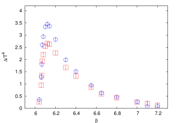
Figure  1.: $\Delta/T^{4}$ as a function of the bare coupling $\beta$ using a non-perturbative (squares) and one-loop order perturbative (pentagons) $\beta$-function, $B(\alpha_{s})$. The results agree for $\beta\geq 6.55$. The plaquette values for $N_{\tau}=8$ and the values of the non-perturbative $\beta$-function are taken from Ref. [2].

While the t-favoured method improves the differential method, leading to positive pressure, it still requires the use of perturbative couplings. On the other hand, the integral method evades them but at the cost of the assumption of homogeneity. For small volumes used in actual simulations, one may feel reassured by its test in form of agreement of results with other methods such as the differential method. Note that the expression for $\Delta/T^{4}$ is identical for both the integral method and the t-favoured scheme. It depends on the $\beta$-function, $B(\alpha_{s})$ in Eq. [18]. A non-perturbatively determined $\beta$-function permits the integral method to lead to fully non-perturbative EOS. However, one usually fits a phenomenological ansatz to extract it from a range of couplings $6/g^{2}$ with their associated systematic uncertainties. The differential method could also employ such a $\beta$-function but for internal consistency we require that the Karsch coefficients and $B(\alpha_{s})$ be obtained at the same order, i.e. at one-loop order in the present state of the art.

The two methods must agree if one uses sufficiently small lattice spacings, viz. when the use of perturbative couplings is justified in the differential method computation and on large enough volumes. A a comparison between the values of $\Delta/T^{4}$ extracted for a given $N_{\tau}$ using the two approaches would reveal at what $T$ the two methods become close to each other. Using asymptotic scaling, one could also then find the minimum value of $N_{\tau}$ required for the same level of agreement as a function of $T$. Such a comparison is shown in Figure 1, which demonstrates that a bare coupling of $\beta\geq 6.55$ should suffice to give an agreement between the t-favoured scheme and the integral method. For $\beta\leq 6.55$ use of one-loop order perturbative Karsch coefficients may give rise to some systematic effects. A comparison with the non-perturbatively determined Karsch coefficients  [?,?] shows that the difference between the perturbative and non-perturbative values are significant. For example, while at around $\beta=6.55$ the one-loop order perturbative and non-perturbative $c_{i}^{\prime}$ differ by $\sim 20\%$, around $\beta=6$ this difference increases to $\sim 80\%$.

In the present work we show that within the framework of differential method it possible to get a positive pressure for all temperatures if one uses the better operators of the t-favoured scheme. This is so in spite of the use of one-loop order perturbative Karsch coefficients. However, the use of one-loop order perturbative Karsch coefficients  [?,?] may give some systematic effects if the lattice spacing is not small enough.

3. Simulations and results

Our simulations have been performed using the Cabbibo-Marinari pseudo-heatbath algorithm with Kennedy-Pendleton updating of three $SU(2)$ subgroups on each sweep. Plaquettes were measured on each sweep. For each simulation we discarded around 5000 initial sweeps for thermalization. We found that the maximum value for the integrated autocorrelation time for the plaquettes is about 12 sweeps for the $T=0$ run at $\beta=6$ and the minimum was 3 sweeps for the $T=3T_{c}$ run for $N_{\tau}=12$. Table 1 lists the details of these runs. All errors were calculated by the jack-knife method, where the length of each deleted block was chosen to be at least six times the maximum integrated autocorrelation time of all the simulations used for that calculation.

In Ref.  [?] it was shown that, at sufficiently high temperature, finite size effects are under control if one chooses $N_{s}=(T/T_{c})N_{\tau}+2$ for the asymmetric ($N_{\tau}\times N_{s}^{3}$) lattice. We have chosen the sizes of the lattices used at finite $T$ based on this investigation. Close to $T_{c}$ the most stringent constraint on allowed lattice sizes comes from the $A_{1}^{++}$ screening mass determined in Ref.  [?]. Among the temperature values we investigated, this screening mass is smallest at $1.25T_{c}$ where it is a little more than $2T$. The choice of $N_{s}=2N_{\tau}+2$ satisfies this constraint sufficiently. If future work pushes closer to $T_{c}$, then larger values of $N_{s}$ need to be used in view of the further decrease in the $A_{1}^{++}$ screening mass. At $T=0$ the constraints are simpler because glueball masses are larger, and also smoother functions of $\beta$. For the symmetric ($N_{s}^{4}$) lattices we have chosen $N_{s}=22$ as the minimum lattice size and scaled this up with changes in the lattice spacing in accordance with the analysis done in Ref.  [?].

Table 1.: The coupling ($\beta$), lattice sizes ($N_{\tau}\times N_{s}^{3}$), statistics and symmetric lattice sizes ($N_{s}^{4}$) are given for each temperature. Statistics means number of sweeps used for measurement of plaquettes after discarding for thermalization.

$T/T_{c}$	$\beta$		Asymmetric Lattice		Symmetric Lattice
		size	stat.	size	stat.
	6.0000	$8\times 18^{3}$	1565000	$22^{4}$	253000
0.9	6.1300	$10\times 22^{3}$	725000	$22^{4}$	543000
	6.2650	$12\times 26^{3}$	504000	$26^{4}$	256000
	6.1250	$8\times 18^{3}$	1164000	$22^{4}$	253000
1.1	6.2750	$10\times 22^{3}$	547000	$22^{4}$	280000
	6.4200	$12\times 26^{3}$	212000	$26^{4}$	136000
	6.2100	$8\times 18^{3}$	1903000	$22^{4}$	301000
1.25	6.3600	$10\times 22^{3}$	877000	$22^{4}$	217000
	6.5050	$12\times 26^{3}$	390000	$26^{4}$	240000
	6.3384	$8\times 18^{3}$	1868000	$22^{4}$	544000
1.5	6.5250	$10\times 22^{3}$	1333000	$22^{4}$	605000
	6.6500	$12\times 26^{3}$	882000	$26^{4}$	335000
	6.5500	$8\times 18^{3}$	2173000	$22^{4}$	534000
2.0	6.7500	$10\times 22^{3}$	1671000	$22^{4}$	971000
	6.9000	$12\times 26^{3}$	1044000	$26^{4}$	553000
	6.9500	$8\times 26^{3}$	1300000	$26^{4}$	433000
3.0	7.0500	$10\times 32^{3}$	563000	$32^{4}$	148000
	7.2000	$12\times 38^{3}$	317000	$38^{4}$	60000

We performed $a\to 0$ (continuum) extrapolations by linear fits in $a^{2}\propto 1/N_{\tau}^{2}$ at all temperatures using the three values $N_{\tau}=8$, 10, and 12. In Figure 2(a) we show our data on $P/T^{4}$ at finite lattice spacings and the continuum extrapolations for different temperatures, both above and below $T_{c}$. We draw attention to the fact that the pressure is positive on each of the lattices we have used and also in the $a\to 0$ limit. It is an interesting piece of lattice physics, not relevant to the continuum limit, that the slope of the continuum extrapolation changes sign at $T_{c}$. This is also true of the continuum extrapolation for $\epsilon/T^{4}$ as shown in Figure 2(b). The extrapolation of both $P/T^{4}$ and $\epsilon/T^{4}$ between $1.1T_{c}$ and $3T_{c}$ are similar to those shown and have therefore been left out of the figure to avoid clutter.

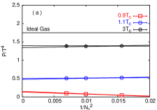
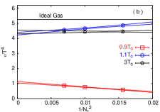
Figure  2.: In the panel (a) we show the dependence of $P/T^{4}$ on $1/N_{\tau}^{2}$ for different temperature values. In the panel (b) we show the same for $\epsilon/T^{4}$. The 1-$\sigma$ error band of the continuum extrapolations have been indicated by the lines.

Similar continuum extrapolations are shown for $C_{\scriptscriptstyle V}/T^{3}$ and $C_{s}^{2}$ in the two panels of Figure 3. In all cases, the continuum extrapolations are smooth, and well fitted by a straight line in the range of $N_{\tau}$ used in this study. As mentioned above, it is interesting lattice physics to see that for $C_{\scriptscriptstyle V}/T^{3}$ also, the slope of the continuum extrapolation flips sign at $T_{c}$. This does not happen for $C_{s}^{2}$. Since this is the derivative of the energy density with respect to the pressure, the slope of this quantity depends on the slopes of the continuum extrapolation of $\epsilon/T^{4}$ and $P/T^{4}$.

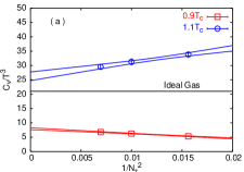
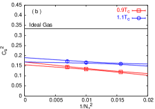
Figure  3.: In the panel (a) we show the dependence of $C_{\scriptscriptstyle V}/T^{3}$ on $1/N_{\tau}^{2}$ for different values of temperature. In the panel (b) we show the same for $C_{s}^{2}$. The 1-$\sigma$ error band of the continuum extrapolations have been indicated by the lines.

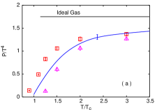
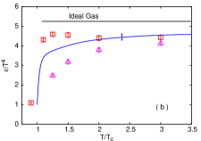
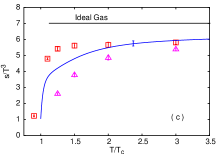
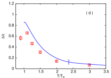
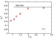
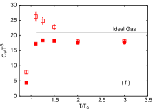
Figure  4.: We show comparisons between the continuum extrapolated results of different thermodynamic quantities for t-favoured scheme (boxes), the s-favoured scheme (triangles) and the integral method (line). In panel (d) we show the continuum extrapolated values of the conformal measure ${\cal C}$ (boxes). In panel (f) we show a comparison between our continuum extrapolated results for $C_{\scriptscriptstyle V}/T^{3}$ (open boxes) and that of $4\epsilon/T^{4}$ (filled boxes). The data for the integral method has been taken form Ref. [2].

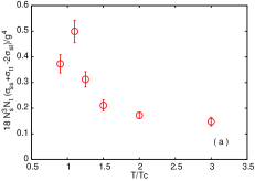
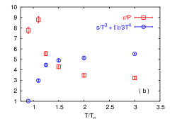
Figure  5.: In panel (a) we show the temperature dependence of the contribution of one of the covariance terms in $C_{\scriptscriptstyle V}/T^{3}$. In panel (b) we show the the individual contribution of the two factors in Eq. (23) for $C_{\scriptscriptstyle V}/T^{3}$. See the text for a detailed discussion.

The results of continuum extrapolations of our measurements are collected in Table 2. It is gratifying to note that the pressure and the entropy are not only positive in the full temperature range, but also convex functions of $T$, as required for thermodynamic stability.

In the various panels of Figure 4 we show a comparison between the continuum extrapolated results for different quantities obtained using the t-favoured scheme, s-favoured scheme and the integral method. While the results of the t-favoured and the s-favoured schemes are obtained from the analysis of our data, the results of the integral method are taken form Ref.  [?].

First we note that unlike the s-favoured differential method, the t-favoured scheme yields a positive pressure [Figure 4(a)] at all $T$. There is apparent agreement between the integral and the t-favoured operator method for $T\geq 2T_{c}$, both differing from the ideal value by about 20%. Only at these temperatures the coupling $\beta$ becomes $\geq 6.55$ for all the lattices (see Table 1) that has been used to extract the continuum extrapolated values in the t-favoured scheme. Hence, from our earlier discussion it is clear that an agreement between the two methods is expected to take place at these temperatures. There can be several causes for the difference between these two methods closer to $T_{c}$— (i) The use of one-loop order perturbative Karsch coefficients in the t-favoured scheme is probably the primary cause for this difference. Use of larger lattices (i.e. larger $\beta$) or inclusion of the effects of higher order loops in the Karsch coefficients is expected to improve the agreement. (ii) Another possible source of disagreement is that the results for the integral method shown here were obtained on coarser lattices  [?] than the ones used in this study. (iii) The integral method assumes that the pressure below some $\beta_{0}$, corresponding to some temperature $T<T_{c}$, is zero. By changing $\beta_{0}$ one can change the integral method pressure by a temperature independent constant. This may restore the agreement close to $T_{c}$, although in that case the agreement at the high-$T$ region may get spoiled. (iv) Also different schemes have been used to define the renormalized coupling in the two cases. This can also make some contribution to the different results of the two methods.

Correspondingly, the energy density is harder near $T_{c}$, showing a significantly lessened tendency to bend down. This could indicate a difference in the latent heat determined by the two methods. We shall return to this quantity in the future. The entropy density is shown in Figure 4(c). Since this is a derived quantity (see Eq. 6), it has similar features as those of $P/T^{4}$ and $\epsilon/T^{4}$.

The generation of a scale and the consequent breaking of conformal invariance at short distances, of the order of $a$, in QCD is, of course, quantified by the $\beta$-function of QCD. It has been argued in Ref.  [?], that the conformal measure, ${\cal C}=\Delta/\epsilon$, parametrizes the departure from the conformal invariance at the distance scale of order $1/T$. In Figure 4(d) we plot $\cal C$. It is clear that at high temperature, 2–3$T_{c}$, conformal invariance is better respected in the finite temperature effective long-distance theory. Closer to $T_{c}$ conformal symmetry is badly broken even in the thermal effective theory. This is consistent with the existence of many mass scales in the theory as found in Ref.  [?,?,?]. It is interesting to note that the t-favoured scheme yields marginally smaller values of $\cal C$ than the integral method. Note also the peak in $\cal C$ just above $T_{c}$; this is the reflection of a similar peak in $\Delta$.

Figure 4(e) shows the continuum extrapolated results for $C_{s}^{2}$. At temperatures of $2T_{c}$ and above, the speed of sound is consistent with the ideal gas value within 95% confidence limits. It is seen that $C_{s}^{2}$ decreases dramatically near $T_{c}$. Below $T_{c}$ there is again a rise in $C_{s}^{2}$, the numerical values being very close 10% below and above $T_{c}$. In future we plan to explore in greater detail the region in between.

The behaviour of $C_{\scriptscriptstyle V}/T^{3}$, shown in Figure 4(f), is the most interesting. At $2T_{c}$ and above it disagrees strongly with the ideal gas value, but is quite consistent with the prediction in conformal theories that $C_{\scriptscriptstyle V}/T^{3}=4\epsilon/T^{4}$. Closer to $T_{c}$, however, even this simplification vanishes. The specific heat peaks at $T_{c}$, consistent with the observation of Refs.  [?,?] that there is a light mode (the thermal scalar, called the $A_{1}^{++}$) in the vicinity of $T_{c}$. Below $T_{c}$ the specific heat is very small.

In view of the rise in $C_{\scriptscriptstyle V}/T^{3}$ near $T_{c}$, we studied the contributions of the terms containing different covariances of the plaquettes. As can be seen from the Eqs. (43, 47), among all the terms containing covariances, the term $(\sigma_{ss}+\sigma_{\tau\tau}-2\sigma_{s\tau})/g^{4}$ will have the largest contribution to $C_{\scriptscriptstyle V}/T^{3}$. All the other terms containing the covariances are multiplied either by one of the $c_{i}^{\prime}$, or by $B(\alpha_{s})/2\pi\alpha_{s}^{2}$ and hence become at least one order of magnitude smaller than this term.

In Figure 5(a) we show the contribution of the above term, as a function of $T$ in the continuum limit. It peaks near $T_{c}$, consistent with the decrease of the $A_{1}^{++}$ screening mass mentioned earlier. Since the lattices that we used are significantly larger than this correlation length, we are in the correct regime of volumes where the central limit theorem holds for the fluctuations of the plaquettes. The contribution of this term is very small: comparable to the errors in $C_{\scriptscriptstyle V}$. The origin of the peak in $C_{\scriptscriptstyle V}$ therefore lies elsewhere. In Figure 5(b) we separately plot the two factors, $\epsilon/P$ and $s/T^{3}+\Gamma\epsilon/3T^{4}$, in the the expression for $C_{\scriptscriptstyle V}$ in Eq. 23. The factor $s/T^{3}+\Gamma\epsilon/3T^{4}$ is smooth in the whole temperature range, and it is the first factor, $\epsilon/P$, which has a peak near $T_{c}$. Rewriting this as $3/(1-{\cal C})$, we can recognize that the peak in $C_{\scriptscriptstyle V}$ is related to that in $\Delta$.

4. Discussion

Table 2.: Continuum values of some quantities at all temperatures we have explored. The numbers in brackets are the error on the least significant digit. For the convenience of the readers here we also list the numerical values of these quantities for an ideal gas— $\epsilon/T^{4}\approx 5.26$, $P/T^{4}\approx 1.75$, $s/T^{3}\approx 7.02$, $C_{\scriptscriptstyle V}/T^{3}\approx 21.06$ and $C_{s}^{2}=1/3$. The value of the ’t Hooft coupling $g^{2}N_{c}$ is computed at the scale $2\pi T$ using the $T_{c}/\Lambda_{\overline{\scriptscriptstyle MS}}$ quoted in Ref. [32].

$T/T_{c}$	$g^{2}N_{c}$	$\epsilon/T^{4}$	$P/T^{4}$	$s/T^{3}$	$C_{\scriptscriptstyle V}/T^{3}$	$C_{s}^{2}$
0.9	11.5(3)	1.09(4)	0.14(1)	1.23(5)	8.0(5)	0.162(7)
1.1	10.4(2)	4.31(9)	0.49(1)	4.80(6)	26(2)	0.18(1)
1.25	9.8(2)	4.6(1)	0.82(2)	5.4(1)	25(1)	0.21(1)
1.5	9.0(1)	4.5(1)	1.06(4)	5.6(2)	22.8(7)	0.25(1)
2.0	8.1(1)	4.4(1)	1.26(4)	5.7(2)	17.9(7)	0.31(1)
3.0	7.0(1)	4.4(1)	1.37(3)	5.8(1)	17.9(8)	0.32(1)

In this paper we have proposed a modification, viz. the t-favoured scheme, of the differential method for the computation of the QCD equation of state. We have shown that this improvement gives positive pressure for all temperatures and $N_{\tau}$ used, even when the older s-favoured differential method  [?] gives negative pressure. Note that this is so in spite of the use of the same one-loop order perturbative values for the couplings in both cases. Using the t-favoured differential method and by extrapolating to the $a\to 0$ (continuum) limit we obtain the energy density and pressure for a pure gluonic theory in the temperature range $0.9\leq T/T_{c}\leq 3$. These differ from their respective ideal gas values by about 20% at $3T_{c}$, and by much more as one approaches $T_{c}$. On comparing our results with those of the integral method  [?], we found that ours are larger for $T<2T_{c}$. The primary reason behind this disagreement seems to be our use of perturbative couplings. Hence the agreement between the t-favoured scheme and the integral method is expected to improve by going to larger temporal lattice sizes or equivalently to smaller lattice spacings.

We have also extended the t-favoured scheme to compute the continuum extrapolated results of the specific heat at constant volume and the speed of sound. We found that $C_{\scriptscriptstyle V}$ peaks near $T_{c}$ where, in addition, $C_{s}$ becomes small. Our results are collected together in Table 2 and Figure 4. The most robust quantity on the equation of state in all lattice computations is $\Delta$, and the most interesting (and also stable) feature seen to date is the peak in $\Delta$ just above $T_{c}$. Apart from influencing the EOS, it manifests itself as a peak in $C_{\scriptscriptstyle V}$. Since $C_{\scriptscriptstyle V}$ could be directly measurable through energy or effective temperature fluctuations in heavy-ion collisions, understanding $\Delta$ should be one of the prime goals of theory. Unfortunately, it seems that at present no tool other than lattice computations are available for this task. Even models of this important and stable phenomenon are lacking.

In view of the fact the perturbation theory fails to reproduce the lattice data on EOS, specially close to $T_{c}$, it is interesting to compare our t-favoured scheme results with that of the perturbation theory. In Figure 6(a) we compare the pressure obtained in the t-favoured method with that from a dimensionally reduced theory, matched with the 4-d theory perturbatively up to order $g^{6}\ln(1/g)$  [?]. Writing $P_{SB}$ for the ideal gas (Stefan-Boltzmann) value of the pressure, the ratio for $P/P_{SB}$ found in the dimensionally reduced theory  [?] has an undetermined adjustable constant, $c$. The pressure determined through dimensional reduction agrees with our results almost all the way down to $T_{c}$, for that value of the constant ($c=0.7$) for which it matches with the integral method in the high temperature range. In future it would be interesting to check whether an equally good description is available in this approach for the full entropy. This would be a non-trivial extension because perturbation theory misses $\Delta$ completely. The question, therefore, addresses the non-perturbative dynamics of the dimensionally reduced theory.

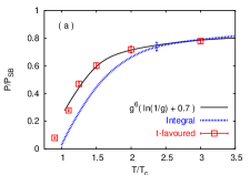
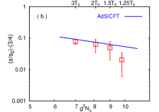
Figure  6.: In panel (a) we compare the pressures obtained by t-favoured method (boxes), integral method (dotted line) and the $g^{6}\ln(1/g)$ order perturbative expansion (solid line) of The data for the integral method and the perturbative expansion are taken from Ref. [2] and Ref. [40] respectively. The values of the $T/\Lambda_{\overline{\scriptscriptstyle MS}}$ in Ref. [40] has been converted to $T/T_{c}$ using the $T_{c}/\Lambda_{\overline{\scriptscriptstyle MS}}$ quoted in Ref. [32]. In panel (b) we show the deviation of $s/s_{0}$ from $3/4$ (boxes) as a function of the ’t Hooft coupling. We also show the prediction of Eq. (1) (solid line).

The strong coupling result in Eq. (2) of Ref.  [?] can be compared with our data on the entropy density, $s/T^{3}$. This has to be done in an appropriate window of $T$ where the ’t Hooft coupling $g^{2}N_{c}$ is large and $\cal C$ is small. The strong coupling series is an expansion in $(g^{2}N_{c})^{-1/2}$. For $N=4$ SYM, the first term vanishes due to a delicate cancellation and the series starts with the $(g^{2}N_{c})^{-3/2}$ term  [?]. When some of the supersymmetry is broken, this cancellation need not occur and the series could start with a term in $(g^{2}N_{c})^{-1/2}$. Needless to say, the theory we are studying here, pure QCD, lacks supersymmetry. In Figure 6(b) we show the deviation of $s/s_{0}$ from $3/4$ as a function of the ’t Hooft coupling ($s$ and $g^{2}N_{c}$ are listed in Table 2). Also shown is the prediction of Eq. (2). Comparison of our data with the latter shows that the AdS/CFT based theory agrees with our data for $g^{2}N_{c}<9$, or in other words for ${\cal C}<0.3$. As a partial summary of our results, we show the equation of state in Figure 7 in the form of a plot of $P/T^{4}$ against $\epsilon/T^{4}$, useful for hydrodynamics. In this plot, the ideal gas for fixed number of colours is represented by a single point which is independent of $T$, and theories with conformal symmetry by the line $\epsilon=3P$. Pure gauge QCD lies close to the conformal line at high temperature, as shown, but deviates strongly nearer $T_{c}$.

The slope of the wedges piercing the ellipses indicates the speed of sound— when these are parallel to the conformal line then $C_{s}^{2}=1/3$. This is clearly the case at high temperature. However, there is an increasing flattening of the axis, denoting a drop in $C_{s}^{2}$ as one approaches $T_{c}$. Note that the slope of the curve joining the middle points of the ellipses does not give $C_{s}^{2}$, since the plot is of $\epsilon/T^{4}$ against $P/T^{4}$. In a plot of $\epsilon$ against $P$, it would have been correct to assume that the slope gives $C_{s}^{2}$.

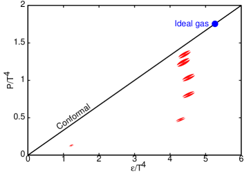
Figure  7.: The equation of state of QCD matter. The diagonal line denotes possible EOS for theories with conformal symmetry. The circle on the diagonal denotes the ideal gluon gas, whose EOS in this form is temperature independent. The ellipses denote 66% error bounds on the measured EOS (see Ref. [41]). The ratio of the axes is a measure of the covariance in the measurements of $\epsilon/T^{4}$ and $P/T^{4}$. The wedges piercing these ellipses have average slope $C_{s}^{2}$, and the opening half-angle of these wedges indicate the error in $C_{s}^{2}$.

Two other physically important effects can be read off the figure. First, the softening of the equation of state just above $T_{c}$ is shown by the rapid drop in pressure at roughly constant $\epsilon/T^{4}$. Second, a large latent heat is indicated by the jump between the last two points, at almost the same pressure but very different energy densities.

A final piece of physics can be deduced from the fact that the low temperature phase shows a very small $P/T^{4}$ at a significantly large value of $\epsilon/T^{4}>1$ just below $T_{c}$. This is an indication that there are very massive modes in the hadron gas which contribute large amounts to $\epsilon$ without contributing to $P$. The small value of $C_{\scriptscriptstyle V}/T^{3}$ at the same $T$ also indicates that the energy required to excite the next state is rather large. We have mentioned already that the observations just above $T_{c}$ are compatible with the known spectrum of excitations in pure gauge QCD  [?].

A Discussion on the Karsch coefficients

The Karsch coefficients ($c_{i}$) are differences between the anisotropic and isotropic lattice couplings and hence do not depend on the scale $a$ of the isotropic lattice, but only on the the anisotropic parameter $\xi$. One can see this directly from the derivations in Ref.  [?], where these have been evaluated up to one-loop order in the perturbation theory. For any arbitrary $\xi\neq 1$, all integrals contributing in the effective action $S_{eff}(a,\xi)$, mentioned in Eq. (2.22) of Ref.  [?], are independent of the scale the $a$. The dependence of $a$ are only encoded implicitly in the couplings $g_{i}^{-2}(a,\xi)$. Hence $S_{eff}(a,\xi)$ of Eq. (2.22) of Ref.  [?] is equally valid for $a=a_{\tau}$. The values of the Karsch coefficients have been evaluated by imposing the condition $\Delta S_{eff}=S_{eff}(a,\xi)-S_{eff}(a,1)=0$, which is again independent of the scale $a$. Hence the one-loop order Karsch coefficients for both the case $a=a_{s}$ ($s-$favoured scheme) and $a=a_{\tau}$ ($t-$favoured scheme) are the same.

Nevertheless, we derive this equality explicitly in the following. Let us assume that the one-loop order perturbative expansions for $g_{i}^{2}$’s, around the isotropic lattice coupling $g$, have the following forms

$$g_{i}^{-2}(a_{s},\xi) = g^{-2}(a_{s})+c_{i}(\xi)+O[g^{2}(a_{s})],\qquad{\rm and}$$ (A1)

$$g_{i}^{-2}(a_{\tau},\xi) = g^{-2}(a_{\tau})+\alpha_{i}(\xi)+O[g^{2}(a_{\tau})].$$ (A2)

Our claim is that $\left[\partial c_{i}(\xi)/\partial\xi\right]_{a_{s}}=\left[\partial\alpha_{i}(\xi)/\partial\xi\right]_{a_{\tau}}$. In order to prove it we make a Taylor series expansion of $g_{i}(a_{s},\xi)$ around $a_{s}=a_{\tau}$, at any fixed $\xi\neq 1$

$$g_{i}^{-2}(a_{s},\xi)=g_{i}^{-2}(a_{\tau},\xi)+\sum_{n=1}^{\infty}\frac{(a_{s}-a_{\tau})^{n}}{n!}\left[\left.\frac{\partial^{n}g_{i}^{-2}(x,\xi)}{\partial x^{n}}\right|_{\xi}\right]_{x=a_{\tau}}.$$ (A3)

A $\xi$ derivative at constant $a_{s}$, on Eq. (A3) yields

$$\left.\frac{\partial g_{i}^{-2}(a_{s},\xi)}{\partial\xi}\right|_{a_{s}} = \left.\frac{\partial g_{i}^{-2}(a_{\tau},\xi)}{\partial\xi}\right|_{a_{s}}+\sum_{n=1}^{\infty}\frac{na_{s}^{n}}{n!\xi^{2}}\left(1-\frac{1}{\xi}\right)^{n-1}\left.\frac{\partial^{n}g_{i}^{-2}(a_{\tau},\xi)}{\partial a_{\tau}^{n}}\right|_{\xi}$$ (A4)

$$+ \sum_{n=1}^{\infty}\frac{a_{s}^{n}}{n!}\left(1-\frac{1}{\xi}\right)^{n}\frac{\partial}{\partial\xi}\left[\left.\frac{\partial^{n}g_{i}^{-2}(a_{\tau},\xi)}{\partial a_{\tau}^{n}}\right|_{\xi}\right]_{a_{s}}.$$ (A5)

While $\left[\partial g(a_{s})/\partial\xi\right]_{a_{s}}=0$, $\left[\partial g(a_{\tau})/\partial\xi\right]_{a_{s}}=\left[\partial g(a_{s}/\xi)/\partial\xi\right]_{a_{s}}\neq 0$, from Eq. (A2) it follows that

$$\left.\frac{\partial g_{i}^{-2}(a_{\tau},\xi)}{\partial\xi}\right|_{a_{s}} = \left.\frac{\partial g^{-2}(a_{\tau})}{\partial\xi}\right|_{a_{s}}+\left.\frac{\partial\alpha_{i}(\xi)}{\partial\xi}\right|_{a_{s}}$$ (A6)

$$= \frac{\partial}{\partial\xi}\left[g^{-2}(a_{s})+\sum_{n=1}^{\infty}\frac{(a_{\tau}-a_{s})^{n}}{n!}\frac{\partial^{n}g^{-2}(a_{s})}{\partial a_{s}^{n}}\right]_{a_{s}}+\left.\frac{\partial\alpha_{i}(\xi)}{\partial\xi}\right|_{a_{s}}$$ (A7)

$$= -\sum_{n=1}^{\infty}\frac{na_{s}^{n}}{n!\xi^{2}}\left(\frac{1}{\xi}-1\right)^{n-1}\frac{\partial^{n}g^{-2}(a_{s})}{\partial a_{s}^{n}}+\left.\frac{\partial\alpha_{i}(\xi)}{\partial\xi}\right|_{a_{s}}.$$ (A8)

Substituting Eq. (A8) in Eq. (A5) and using relations in Eq. (A2) to calculate the various derivatives one obtains

$$\left.\frac{\partial c_{i}(\xi)}{\partial\xi}\right|_{a_{s}} = -\sum_{n=1}^{\infty}\frac{na_{s}^{n}}{n!\xi^{2}}\left(\frac{1}{\xi}-1\right)^{n-1}\frac{\partial^{n}g^{-2}(a_{s})}{\partial a_{s}^{n}}+\left.\frac{\partial\alpha_{i}(\xi)}{\partial\xi}\right|_{a_{s}}$$ (A9)

$$+ \sum_{n=1}^{\infty}\frac{na_{s}^{n}}{n!\xi^{2}}\left(1-\frac{1}{\xi}\right)^{n-1}\left.\frac{\partial^{n}g^{-2}(a_{\tau})}{\partial a_{\tau}^{n}}\right|_{\xi}$$ (A10)

$$+ \sum_{n=1}^{\infty}\frac{a_{s}^{n}}{n!}\left(1-\frac{1}{\xi}\right)^{n}\frac{\partial}{\partial\xi}\left[\frac{\partial^{n}g^{-2}(a_{\tau})}{\partial a_{\tau}^{n}}\right]_{a_{s}}.$$ (A11)

Finally, taking the $\xi\to 1$ limit, i.e. setting $a_{s}=a_{\tau}$, one has

$$\left.\frac{\partial c_{i}(\xi)}{\partial\xi}\right|_{a_{s}}=\left.\frac{\partial\alpha_{i}(\xi)}{\partial\xi}\right|_{a_{s}}$$ (A12)

A variable transformation from $\{a_{s},\xi\}$ to $\{a_{\tau},\xi\}$ gives $\xi\left(\partial/\partial\xi\right)_{a_{s}}\equiv\xi\left(\partial/\partial\xi\right)_{a_{\tau}}-a_{\tau}\left(\partial/\partial a_{\tau}\right)_{\xi}$. Using it on Eq. (A12) one conclusively proves that

$$\left.\frac{\partial c_{i}(\xi)}{\partial\xi}\right|_{a_{s}}=\left.\frac{\partial\alpha_{i}(\xi)}{\partial\xi}\right|_{a_{\tau}}$$ (A13)

REFERENCES

-
[1]
K. Adcox et al.[PHENIX Collaboration], Nucl. Phys. A 757, 184 (2005);
I. Arsene et al.[BRAHMS collaboration], Nucl. Phys. A757, 1 (2005);
B. B. Back et al.[PHOBOS collaboration], Nucl. Phys. A 757, 28 (2005);
J. Adams et al.[STAR Collaboration], Nucl. Phys. A 757, 102 (2005). - [2] G. Boyd et al., Phys. Rev. Lett. 75, 4169 (1995); Nucl. Phys. B 469, 419 (1996).
- [3] R. V. Gavai, S. Gupta and S. Mukherjee, Phys. Rev. D 71, 074013 (2005).
- [4] S. Gupta, Phys. Lett. B 597, 57 (2004).
- [5] S. Gupta, Pramana 61, 877 (2003).
-
[6]
P. Arnold and C. Zhai, Phys. Rev. D 50, 7603 (1994); ibid.
D 51, 1906 (1995);
E. Braaten and A. Nieto, Phys. Rev. D 53, 3421 (1996);
K. Kajantie et al., Phys. Rev. Lett. 86, 10 (2001); J. H. E. P. 0304, 036 (2003). - [7] A. Peshier, Nucl. Phys. A 702, 128 (2002).
-
[8]
J. O. Andersen et al., Phys. Rev. D 66, 085016 (2002);
J.-P. Blaizot, E. Iancu and A. Rebhan, Phys. Rev. D 63, 065003(2001);
K. Kajanie et al., Phys. Rev. Lett. 86, 10 (2001). - [9] A. Dumitru, J. Lenaghan and R. D. Pisarski, Phys. Rev. D 71, 074004 (2005).
- [10] B. Grossman et al., Nucl. Phys. B 417, 289 (1994).
- [11] K. Kajantie et al., Phys. Rev. Lett. 79, 3130 (1997).
- [12] S. Datta and S. Gupta, Nucl. Phys. B 534, 392 (1998).
- [13] M. Laine and O. Philipsen, Phys. Lett. B 459, 259 (1999).
- [14] S. Datta and S. Gupta, Phys. Rev. D 67, 054503 (2003).
- [15] A. Hart, M. Laine and O. Philipsen, Nucl. Phys. B 586, 443 (2000).
- [16] P. de Forcrand et al.[QCD-TARO Collaboration], Phys. Rev. D 63, 054501 (2001).
-
[17]
S. S. Gubser, I. R. Klebanov and A. A. Tseytlin, Nucl. Phys. B 534,
202 (1998);
I. R. Klebanov, hep-th/0009139. - [18] P. Kovtun, D. T. Son and A. Starinets, J. H. E. P. 0310, 064 (2003).
- [19] D. Teaney, Phys. Rev. C 68, 034913 (2003).
- [20] A. Nakamura and S. Sakai, Phys. Rev. Lett. 94, 072305 (2005).
- [21] H. B. Meyer, Phys. Rev. D 76, 101701 (2007), ibid. arXiv:0710.3717 [hep-lat].
- [22] J. Engels et al., Nucl. Phys. B 205 [FS5], 545 (1982).
- [23] Y. Deng, Nucl. Phys. B (Proc. Suppl.) 9, 334 (1989).
- [24] J. Engels, J. Fingberg, F. Karsch, D. Miller and M. Weber, Nucl. Phys. B 252, 625 (1990).
- [25] W. H. Press et al., Numerical Recipes (Cambridge University Press, Cambridge, 1986.)
- [26] S. Ejiri, Y. Iwasaki and K. Kanaya, Phys. Rev. D 58, 094505 (1998).
- [27] L. Stodolsky, Phys. Rev. Lett. 75, 1044 (1995).
- [28] R. S. Bhalerao, J. P. Blaizot, N. Borghini and J. Y. Ollitrault, Phys. Lett. B 627, 49 (2005).
- [29] See, for example, L. D. Landau and E. M. Lifschitz, Fluid Mechanics , (Reed Elsevier plc, Oxford, 1998), p. 254.
- [30] R. V. Gavai and A. Gocksch, Phys. Rev. D 33, 614 (1986).
- [31] See, for example, S. Aoki et al., Nucl. Phys. (Proc. Suppl.) B 106, 477 (2002).
- [32] A. Hasenfratz and P. Hasenfratz, Nucl. Phys. B 193, 210 (1981).
- [33] F. Karsch, Nucl. Phys. B 205 [FS5], 285 (1982).
- [34] S. Datta and R. V. Gavai, Phys. Rev. D 60, 034505 (1999).
- [35] S. Gupta, Phys. Rev. D 64, 034507 (2001).
- [36] G. P. Lepage and P. B. Mackenzie, Phys. Rev. D 48, 2250 (1993).
- [37] R. G. Edwards, U. M. Heller and T. R. Klassen, Nucl. Phys. B 517, 377 (1998).
- [38] U. M. Heller and F. Karsch, Nucl. Phys. B 251 [FS13], 254 (1985).
- [39] We thank Kari Rummukainen, Keijo Kajantie and Jürgen Engels for discussions on this point.
- [40] J. Engels, F. Karsch and T. Scheideler, Nucl. Phys. B 564, 303 (2000).
- [41] S. Datta and S. Gupta, Phys. Lett. B 471, 382 (2000).
- [42] O. Kaczmarek et al., Phys. Rev. D 62, 034021 (2001).
- [43] K. Kajantie et al., Phys. Rev. D 67, 105008 (2003).
- [44] L. Lyons, Statistics for nuclear and particle physicists , (Cambridge University Press, Cambridge, 1992.)