Perturbative Study of the Supersymmetric Lattice Theory from Matrix Model

Abstract

We study the lattice model for the supersymmetric Yang-Mills theory in two-dimensions proposed by Cohen, Kaplan, Katz, and Unsal. We re-examine the formal proof for the absence of susy breaking counter terms as well as the stability of the vacuum by an explicit perturbative calculation for the case of $U(2)$ gauge group. Introducing fermion masses and treating the bosonic zero momentum mode non-perturbatively, we avoid the infra-red divergences in the perturbative calculation. As a result, we find that there appear mass counter terms for finite volume which vanish in the infinite volume limit so that the theory needs no fine-tuning. We also find that the supersymmetry plays an important role in stabilizing the lattice spacetime by the deconstruction.

I Introduction

The lattice field theory methods are expected to be useful for the non-perturbative study of supersymmetric gauge theories, but a satisfactory formulation which can be applied to efficient simulation has not been obtained so far despite much effort in the study of supersymmetric lattice formulations (see  Kaplan2 -Neuberger 98 ). Since the supersymmetry algebra contains infinitesimal translations, it is quite difficult to construct a lattice theory without an explicit breaking of the supersymmetry due to the lattice regularization, which in principle gives rise to all possible supersymmetry breaking terms not prohibited by other symmetries at the quantum level. This makes practical non-perturbative simulations extremely difficult due to too many parameters which requires fine-tuning in order to recover the supersymmetry in the continuum limit.

To solve this problem, one of the promising approaches is to construct the lattice formulations preserving partial exact supersymmetry . Cohen-Kaplan-Katz-Unsal(CKKU) Kaplan2 ; Kaplan1 ; Kaplan3 ; Kaplan:2005ta constructed a matrix model realization of such theories based on the orbifolding Orbifold1 ; Orbifold2 and deconstruction deconstruction1 ; deconstruction2 method. The first non-perturbative studies of these CKKU models are performed by Giedt Giedt 0304 -Giedt 0405 . Orbifolding is the projection of the zero-dimensional or one-dimensional matrix models by some discrete subgroup of the symmetry. A zero-dimensional moose diagram which is regarded as lattice structure is obtained by this procedure. Supercharges which are invariant under the orbifold projection becomes the symmetry on the lattice. In these procedures, one can make lattice models with an exact partial supersymmetry if one chooses appropriate generators for orbifold projection. Deconstruction is a dynamical construction of the $d$-dimensional spacetime on a $N^{d}$ lattice with the spontaneous symmetry breakdown of the gauge symmetry of the moose diagram $U(M)^{N^{d}}\rightarrow U(M)_{diag}$. In this model, they apply the deconstruction at the zero-dimensional moose diagram.

One possible problem in this approach is that the extended supersymmetry has flat directions for the scalar so that the lattice structure from the deconstruction suffers from the instability due to the quantum fluctuations of the scalar zero momentum modes. To suppress the divergence in the flat directions, soft susy-breaking terms for the scalar fields are introduced. Since such terms break the supersymmetry and causes the infra-red divergence of fermion zero modes, the original discussion of the renormalization based on exact supersymmetry on the lattice has to be modified by including the breaking terms.

In this paper, we concentrate on the two-dimensional $U(2)$ lattice gauge model of CKKU in Ref. Kaplan2 , and investigate the fine-tuning problem and the stability of the spacetime structure by an explicit calculation of quantum corrections of fields which can be relevant. We calculate the quantum corrections of scalar one-point and two-point functions in the model of Ref. Kaplan2 . Before the explicit calculation, we have to take care of ill-defined perturbation due to the flat directions in the zero momentum modes of gauge fields and fermion fields Giedt 0304 . In order to avoid the infra-red divergence for the fermion zero mode, we introduce a new soft susy breaking mass term for the fermion fields. For the bosonic fields, we apply the perturbation only for the non-zero momentum mode and treat the zero momentum mode non-perturbatively. In addition to the fine-tuning problem, several interesting results are obtained by our explicit calculation. Firstly, we found the constraint for the parameter region where the lattice theory is well-defined. And secondly, it is found that the fermion-boson cancellation which suppresses the quantum corrections to the potential is needed to stabilize the deconstructed spacetime in the physical region where the lattice size is larger than the correlation length. Similar instability has been observed in the non-perturbative study  Giedt 0312 on the bosonic part of the CKKU model for the (4,4) 2d super-Yang-Mills Kaplan3 .

The paper is organized as follows. We review the model by CKKU Kaplan2 in Sec. II. In Sec. III, we explain possible counter terms. We also explain the problem of fermion zero-mode which is called as ‘ever-existing fermion zero mode’. In Sec. IV, we will describe the treatment of massless zero momentum modes which make the perturbative calculation based on the gaussian integral ill-defined. In Sec. V, we present our results on the renormalization of susy breaking counter terms. Sec. VI is devoted to the discussion on the constraint from the stability of the spacetime. Our conclusion and discussions are given in Sec. VII. Technical details such as mathematical notations, path-integral measures, and amplitudes are described in the Appendices.

II Brief review of CKKU model

The model by CKKU Kaplan2 is constructed from the zero-dimensional matrix model with four supercharges,

$$S=\frac{1}{g^{2}}(\frac{1}{4}Trv_{mn}v_{mn}+Tr\bar{\psi}\bar{\sigma}_{m}[v_{m},\psi]),$$ (II.1)

where $\sigma$ is the Pauli matrices, $v_{mn}=[v_{m},v_{n}]$ and $v_{m}=v_{m}^{\alpha}T^{\alpha},\,\psi=\psi^{\alpha}T^{\alpha}$, $T^{\alpha}$ is the generators of $U(MN^{2})$ gauge group, and $g$ is the gauge coupling. The above action is obtained by the dimensional reduction of the 4-dimensional $\mathcal{N}=1$ super-Yang-Mills theory to the zero-dimensional theory. They constructed the lattice structure by imposing the following orbifolding condition on the matrix theory

$$\Phi_{\mu,\nu}=[e^{\frac{2\pi ir_{a}}{N}}\mathcal{C}_{a}\Phi\mathcal{C}_{a}^{-1}]_{\mu,\nu},$$ (II.2)

where $\mu,\nu$ are the indices of the gauge group $U(MN^{2})$. $r_{a}(a=1,2)$ are the generators of the Cartan subalgebra of the R-symmetry $SO(4)\times U(1)$, whereas $\mathcal{C}_{a}$ are generators of a discrete symmetry $Z_{N}\otimes Z_{N}\subset U(MN^{2})$ as given in Ref. Kaplan2 . If we decompose the matrices into $N^{2}\times N^{2}$ blocks of $M\times M$ submatrices, the above orbifolding conditions require that only $N^{2}$ blocks can be non-zero, while the other blocks are projected out. By interpreting the indices for different blocks as the coordinates of the two-dimensional spacetime, we obtain a lattice structure which preserve one of the four supercharges exactly. In this interpretation $N$ is regarded as the number of lattice sites for each directions. The lattice action is

$$S_{0}=\frac{1}{g^{2}}\sum_{\mathbf{n}}Tr[\frac{1}{2}(\bar{x}_{\mathbf{n-i}}x_{\mathbf{n-i}}-x_{\mathbf{n}}\bar{x}_{\mathbf{n}}+\bar{y}_{\mathbf{n-j}}y_{\mathbf{n-j}}-y_{\mathbf{n}}\bar{y}_{\mathbf{n}})^{2}$$

$$+2|x_{\mathbf{n}}y_{\mathbf{n+i}}-y_{\mathbf{n}}x_{\mathbf{n+j}}|^{2}$$

$$+\sqrt{2}(\alpha_{\mathbf{n}}\bar{x}_{\mathbf{n}}\lambda_{\mathbf{n}}-\alpha_{\mathbf{n-i}}\lambda_{\mathbf{n}}\bar{x}_{\mathbf{n-i}})+\sqrt{2}(\beta_{\mathbf{n}}\bar{y}_{\mathbf{n}}\lambda_{\mathbf{n}}-\beta_{\mathbf{n-j}}\lambda_{\mathbf{n}}\bar{y}_{\mathbf{n-j}})$$

$$-\sqrt{2}(\alpha_{\mathbf{n}}y_{\mathbf{n+i}}\xi_{\mathbf{n}}-\alpha_{\mathbf{n+j}}\xi_{\mathbf{n}}y_{\mathbf{n}})+\sqrt{2}(\beta_{\mathbf{n}}x_{\mathbf{n+j}}\xi_{\mathbf{n}}-\beta_{\mathbf{n+i}}\xi_{\mathbf{n}}x_{\mathbf{n}})],$$ (II.3)

where $x_{\mathbf{n}}$, $\bar{x}_{\mathbf{n}}$ and $y_{\mathbf{n}}$, $\bar{y}_{\mathbf{n}}$ are the linear combinations of the submatrices in $v_{1}$, $v_{3}$ and $v_{2}$, $v_{4}$ respectively. $\alpha_{\mathbf{n}}$, $\beta_{\mathbf{n}}$ $\lambda_{\mathbf{n}}$, $\xi_{\mathbf{n}}$ are the submatrices in $\bar{\psi}$ and $\psi$ respectively.

A mechanism called as deconstruction is applied in which the kinetic term is generated by a spontaneous breakdown of the gauge symmetry. The bosonic potential in the action after the orbifolding allows the following classical minimum as vacuum expectation values (VEV) $x_{\mathbf{n}}=y_{\mathbf{n}}=\bar{x}_{\mathbf{n}}=\bar{y}_{\mathbf{n}}=\frac{1}{\sqrt{2}a}\times\mathbf{1}_{k}$ , where $a$ is the lattice spacing. Expanding the bosonic fields around this VEV as

$$x_{\mathbf{n}}=\frac{1}{\sqrt{2}a}\times\mathbf{1}_{k}+\frac{s_{x\mathbf{n}}+iv_{x\mathbf{n}}}{\sqrt{2}}, \bar{x}_{\mathbf{n}}=\frac{1}{\sqrt{2}a}\times\mathbf{1}_{k}+\frac{s_{x\mathbf{n}}-iv_{x\mathbf{n}}}{\sqrt{2}},$$

$$y_{\mathbf{n}}=\frac{1}{\sqrt{2}a}\times\mathbf{1}_{k}+\frac{s_{y\mathbf{n}}+iv_{y\mathbf{n}}}{\sqrt{2}}, \bar{y}_{\mathbf{n}}=\frac{1}{\sqrt{2}a}\times\mathbf{1}_{k}+\frac{s_{y\mathbf{n}}-iv_{y\mathbf{n}}}{\sqrt{2}},$$ (II.4)

the action acquires kinetic terms. Taking a naive $a\to 0$ limit the action can be written as

$$S= \frac{1}{g_{2}^{2}}\int d^{2}xTr\Bigl{(}|D_{m}s|^{2}+\bar{\psi}iD_{m}\gamma_{m}\psi+\frac{1}{4}v_{mn}v_{mn}$$

$$+i\sqrt{2}(\bar{\psi}_{L}[s,\psi_{R}]+\bar{\psi}_{R}[s^{\dagger},\psi_{L}])+\frac{1}{2}[s^{\dagger},s]^{2}\Bigr{)},$$ (II.5)

which is $\mathcal{N}=2$ $U(M)$ super-Yang-Mills theory in two-dimensions. In this paper, we concentrate on $U(2)$ gauge theories. Here $g_{2}=ga$ is the two-dimensional gauge coupling and $s=\frac{s_{x}+is_{y}}{\sqrt{2}}$ and $s^{\dagger}$ is hermitian conjugate of $s$. The definition of the fermion fields and gamma matrices are same as in Ref. Kaplan2 .

In Ref. Kaplan2 , the authors argued that the theory recovers the full supersymmetry without the need for fine-tuning. Let us here repeat their arguments. The counter terms which can appear in the two-dimensional lattice theory have the following form

$$\delta S=\frac{1}{g_{2}^{2}}Tr\int d\theta\int d^{2}x\mathcal{C_{O}O}$$ (II.6)

The mass dimension of coupling $M(g_{2})$ is $M(g_{2})=1$. And $M(\int d^{2}x)=-2$,$M(\int d\theta)=\frac{1}{2}$. If the operator $\mathcal{O}$ has dimension $M(\mathcal{O})=p$, mass dimension of coefficient $\mathcal{C_{O}}$ must be $M(\mathcal{C_{O}})=\frac{7}{2}-p$. In perturbation theory, the coefficient $\mathcal{C_{O}}$ can be expanded as

$$\mathcal{C_{O}}=a^{p-\frac{7}{2}}\sum_{l}c_{l}(g_{2}^{2}a^{2})^{l},$$ (II.7)

where $l$ is the order of loop expansion and $c_{l}$ is the coefficient of $l$-th order. Therefore at $l$-loop, relevant operators must satisfy

$$p\leq\frac{7}{2}-2l$$ (II.8)

At 1-loop level, only operators with dimensions $0\leq p\leq\frac{3}{2}$ are relevant. Beyond 1-loop level, there is no relevant operator, since Eq. (II.8) allows only the negative mass dimensions. The operators which can satisfy this condition are only 1-point function of bosonic super-field $\mathbf{B}$, and 1-point function of fermionic one $\mathbf{F}$. $\mathbf{B}$ cannot give any contributions due to the Grassman parity, $\int d\theta$. There are two candidates $\Lambda$ and $\Xi$ for the fermionic 1-point function, where $\Lambda$ and $\Xi$ are the superfields corresponding to $\lambda$ and $\xi$. Since $\Xi$ is forbidden by $Z_{2}$ point symmetry, the only term which can be relevant is $\Lambda$, however we can ignore this term since it is the cosmological constant. As a result, there is no relevant operator due to supersymmetry and the discrete symmetry on the lattice. This naive power counting arguments give a formal proof for the emergence of the supersymmetry in the continuum limit without fine-tuning. However, we should remark that the above argument assumes that the perturbation theory is well-defined.

The formalism of CKKU also assumes the symmetry breaking for the deconstruction. However as they pointed out, the integral over the zero momentum modes of scalar fields is divergent, since there are flat directions in the action Eq. (II.3). This divergence causes a serious instability of the vacuum. In order to control the stability of the vacuum, they modified the theory and introduced soft scalar mass terms to suppress the divergence,

$$S_{1}=S_{0}+\frac{a^{2}\mu^{2}}{g^{2}}\sum_{\mathbf{n}}Tr[(x_{\mathbf{n}}\bar{x}_{\mathbf{n}}-\frac{1}{2a^{2}})^{2}+(y_{\mathbf{n}}\bar{y}_{\mathbf{n}}-\frac{1}{2a^{2}})^{2}],$$ (II.9)

where they take mass parameter $\mu$ to be inversely proportional to the lattice size $L\equiv Na$. Whether the above formal proof for renormalization remains valid even with the soft susy breaking term should be examined. And also whether the perturbation is well-defined or not should be studied.

III Subtleties in CKKU model

In this section, we consider the subtleties in CKKU theory. In the discussion on the renormalization in the previous section, they assumed that the perturbation theory is well-defined. However after introducing the soft susy breaking terms, there appear infra-red divergences from massless fields which do not cancel with each other. It is therefore important to re-examine the renormalization at 1-loop level by explicit calculations in order to see whether this theory really needs fine-tuning or not.

Since there is no exact supersymmetry in the modified action, we do not exploit the superfield formalism here, so that operators $\mathcal{O}$ in this section do not contain the grassman coordinate $\theta$ any more as opposed to the operators $\mathcal{O}$ in the previous section. Radiative corrections induce the operator $\mathcal{O}$ of the following structure into the action

$$\delta S=\frac{1}{g_{2}^{2}}Tr\int d^{2}z\mathcal{C_{O}}\mathcal{O}.$$ (III.1)

Relevant or marginal operators ($\mathcal{O}$) whose canonical dimension $M[\mathcal{O}]=p$ at the $l$-loop correction must satisfy

$$p\leq 4-2l$$ (III.2)

At 1-loop level, relevant or marginal operators with dimensions $0\leq p\leq 2$ can arise. At 2-loop level, relevant operators with the dimension $p=0$ can arise. Beyond 2-loop, there is no relevant or marginal counter term. Since the operator with the dimension $p=0$ is the cosmological constant, it does not play any serious role in fine-tuning problems.

Let us now focus on the 1-loop relevant or marginal counter-terms. Since bosonic fields have dimension 1 and fermionic fields have dimension $\frac{3}{2}$, the candidates for such operators are bosonic 1-point and 2-point functions. Although fermionic 1-point functions are possible from dimension counting, they are forbidden by Grassman parity.

Since 1-point functions of gauge fields are forbidden from Furry’s theorem and the 2-point ones are also forbidden by the gauge symmetry. Hence the only possible counter terms are

• $<s_{x}>,<s_{y}>$ (scalar 1point functions),

• $<s^{2}_{x}>,<s^{2}_{y}>$ (scalar 2point functions).

In what follows, we will discuss the renormalization of these two operators.

Another subtlety is the existence of an exact zero mode of the fermion matrix called ‘ever-existing zero mode’. It was pointed out by Giedt Giedt 0304 that the constant mode of the $U(1)$ part of the fermion, which is independent of the bosonic field configurations, completely decouples from the theory. Therefore a naive path-integral of this model would be ill-defined, unless one either removes this mode or introduce an infra-red regulator. The existence of this mode can be understood as follows: The fermionic part of the action for the mother theory is

$$S_{F}=\frac{1}{g^{2}}Tr(\bar{\psi}\bar{\sigma}_{m}[v_{m},\psi]),$$ (III.3)

where the fields are described by the adjoint representation of $U(2N^{2})$ gauge group. It is obvious that the $U(1)$ component of $\psi$ is the exact zero mode. Since $\lambda$ in $\psi$ has a neutral charge for the R-symmetry $U(1)_{r_{1}}\times U(1)_{r_{2}}$, The constant mode $Tr_{U(MN^{2})}[\psi^{\alpha}(T^{\alpha})]=\sum_{\mathbf{n}}Tr\lambda^{0}_{\mathbf{n}}$ survives as an exact zero mode in the daughter theory after orbifolding. In this work, to make path-integral well-defined, we propose to introduce the following fermion mass term with coefficient $\mu_{F}$ proportional to $\frac{1}{L}$ so that the action now becomes

$$S_{2} = S_{1}+\frac{a\mu_{F}\sqrt{2}}{g^{2}}Tr\sum_{\mathbf{n}}(\alpha_{\mathbf{n}}\bar{x}_{\mathbf{n}}\lambda_{\mathbf{n}}+\beta_{\mathbf{n}}\bar{y}_{\mathbf{n}}\lambda_{\mathbf{n}}-\alpha_{\mathbf{n}}y_{\mathbf{n+i}}\xi_{\mathbf{n}}+\beta_{\mathbf{n}}x_{\mathbf{n+j}}\xi_{\mathbf{n}}).$$ (III.4)

Note that this mass term (III.4) and the bosonic mass terms (II.9) play slightly different roles. The bosonic term (II.9) gives mass only to scalar fields but not to the gauge fields which are protected by the exact gauge symmetry, while the fermion mass term (III.4) gives masses to all fermion fields including gaugino. This asymmetry causes crucial effects on the quantum corrections as will be explained in the Sec.V.3.2.

IV Calculational methods

IV.1 Parameterization of bosonic fields and gauge fixing

In Ref. Kaplan2 , bosonic fields $s,v$ are defined by the real and imaginary parts of fluctuations of $x,y$ from the (VEV) as in Eq. (II.4). As pointed out in Ref. Unsal , we could instead take the following parameterization to define bosonic fields $s,v$:

$$x_{\mathbf{n}}=\frac{1}{\sqrt{2}}(\frac{1+\langle s\rangle}{a}+s_{x\mathbf{n}})e^{iav_{x\mathbf{n}}}\quad y_{\mathbf{n}}=\frac{1}{\sqrt{2}}(\frac{1+\langle s\rangle}{a}+s_{y\mathbf{n}})e^{iav_{y\mathbf{n}}}$$ (IV.1)

$$\bar{x}_{\mathbf{n}}=\frac{1}{\sqrt{2}}e^{-iav_{x\mathbf{n}}}(\frac{1+\langle s\rangle}{a}+s_{x\mathbf{n}})\quad\bar{y}_{\mathbf{n}}=\frac{1}{\sqrt{2}}e^{-iav_{y\mathbf{n}}}(\frac{1+\langle s\rangle}{a}+s_{y\mathbf{n}}),$$ (IV.2)

where $\langle s\rangle$ represents the shift of the VEV by quantum corrections. This parameterization is convenient since one can separate the gauge transformation property for $s$ and $v$; $s$ transform as adjoint site fields under gauge transformation while $v$ transforms as bifundamental link variable. In the following analysis we adopt the parameterization in Eqs.(IV.1), (IV.2).

We introduce the gauge fixing term:

$$S_{gf}=\frac{1}{2g^{2}}\{\frac{1}{\sqrt{2}}\alpha^{g}\}^{2}\sum_{\mathbf{n}}Tr[\{\nabla_{x}^{-}(x_{\mathbf{n}}-\bar{x}_{\mathbf{n}})+\nabla_{y}^{-}(y_{\mathbf{n}}-\bar{y}_{\mathbf{n}})\}^{2}],$$ (IV.3)

where $\nabla^{\pm}_{x,y}$ are difference operators in the forward or backward directions $\nabla^{\pm}_{x}f_{\mathbf{n}}=\pm\frac{1}{a}\{f_{\mathbf{n}\pm\mathbf{i}}-f_{\mathbf{n}}\}$ ,$\nabla^{\pm}_{y}f_{\mathbf{n}}=\pm\frac{1}{a}\{f_{\mathbf{n}\pm\mathbf{j}}-f_{\mathbf{n}}\}$ and $\alpha^{g}$ is an arbitrary parameter. We take $\alpha^{g}$ as the Feynman gauge $\alpha^{g}=(1+\langle s\rangle)$ which make the propagator of the gauge fields diagonal. From the gauge fixing condition (IV.3) and the notation (IV.1,IV.2), ghost term is expressed as follows.

$$S_{gh}= \frac{1}{2\bar{g}^{2}}(1+<s>)\sum_{\mathbf{n}}Tr[\bar{c}_{\mathbf{n}}(\nabla_{x}^{-}\{i[c_{\mathbf{n}},(\frac{1+\langle s\rangle}{a}+s_{x\mathbf{n}})U_{x\mathbf{n}}]-i(\frac{1+\langle s\rangle}{a}+s_{x\mathbf{n}})U_{x\mathbf{n}}\nabla_{x}^{+}c_{\mathbf{n}}$$

$$-i[c_{\mathbf{n}},U^{\dagger}_{x\mathbf{n}}(\frac{1+\langle s\rangle}{a}+s_{x\mathbf{n}})]-i\nabla_{x}^{+}c_{\mathbf{n}}U^{\dagger}_{x\mathbf{n}}(\frac{1+\langle s\rangle}{a}+s_{x\mathbf{n}})\}$$

$$\nabla_{y}^{-}\{i[c_{\mathbf{n}},(\frac{1+\langle s\rangle}{a}+s_{y\mathbf{n}})U_{y\mathbf{n}}]-i(\frac{1+\langle s\rangle}{a}+s_{y\mathbf{n}})U_{y\mathbf{n}}\nabla_{y}^{+}c_{\mathbf{n}}$$

$$-i[c_{\mathbf{n}},U^{\dagger}_{y\mathbf{n}}(\frac{1+\langle s\rangle}{a}+s_{y\mathbf{n}})]-i\nabla_{y}^{+}c_{\mathbf{n}}U^{\dagger}_{y\mathbf{n}}(\frac{1+\langle s\rangle}{a}+s_{y\mathbf{n}})\}),$$ (IV.4)

where $c_{\mathbf{n}},\bar{c}_{\mathbf{n}}$ are ghost and anti-ghost fields respectively, and $U_{\nu\mathbf{n}}=e^{iav_{\nu\mathbf{n}}}\,(\nu=x,y)$.

IV.2 Treatment of zero momentum modes

In the present theory the coupling $\bar{g}$ is the product of two-dimensional gauge coupling $g_{2}$ and lattice spacing $a$ as $\bar{g}=g_{2}a$. For a fixed gauge coupling $g_{2}$, the dimensionless coupling $\bar{g}$ becomes small near the continuum limit, therefore the perturbation theory is expected to become a good approximation. However, since there is no quadratic term of massless zero momentum modes, perturbative calculations based on the gaussian integral becomes ill-defined, thus a special care must be taken for the zero momentum modes. In our approach, we carry out non-perturbative calculation for the zero momentum modes while non-zero momentum modes are treated perturbatively.

The calculational procedures are the following:

1. We perform the fourier transformation of the fields as given in Appendix. A, including the rescaling of the fields by certain powers in $\bar{g}$ and $N$. $\bar{g},\bar{\mu},\frac{1}{N}$ are used as the parameter for perturbative expansion, where $\bar{\mu}=a\mu=\frac{a}{L}$.

2. We carry out exact fermionic integral for both zero momentum modes and non-zero momentum modes. Then we also carry out 1-loop perturbation for the non-zero momentum bosonic fields.

3. The effective action is the sum of the tree level action for the zero momentum bosonic fields and logarithm of the determinant from the 1-loop integral for other fields which also depends on the zero momentum boson fields. Expanding the 1-loop contribution in terms of the zero momentum boson fields, the leading term is a constant and next leading and next-to-next leading terms are the 1-point and 2-point functions. By the discussion in Sec. III, only these three terms can be relevant and higher terms in the effective action are irrelevant. We show that the 1-point and 2-point functions at the effective potential are irrelevant by explicit calculation, which will be described in Sec. V.3

4. Once the 1-point and 2-point functions in the effective potential are shown to be irrelevant, these terms can be neglected in the effective action. Then the final form of the path-integral over the zero momentum bosonic fields can be reduced into a simpler form. A non-perturbative calculation of the path-integral will be described in Sec. V.4.

V Results

V.1 Procedure 1: Fourier transformation

Let us consider the following 1-point and 2-point functions of the scalar fields $s_{\mu}=s_{\mu}^{\alpha}T^{\alpha}$, where $\mu=x,y$ and $T^{\alpha}(\alpha=0,1,2,3)$ are the generator of $U(2)$ gauge group with $T^{0}=\frac{1}{2}\times\mathbf{1}$ and pauli matrices $T^{a}=\frac{1}{2}\sigma^{a}(a=1,2,3)$ .

$$I^{\alpha}_{1} \equiv \sum_{\mathbf{n}}\langle s^{\alpha}_{\mu\mathbf{n}}\rangle=\frac{\int\displaystyle{\prod_{\beta,\mathbf{n}}}(\displaystyle{\prod_{\nu}}d\phi_{\nu\mathbf{n}}^{\beta})d\psi_{\mathbf{n}}^{\beta}d\bar{\psi}_{\mathbf{n}}^{\beta}det^{\prime}(D_{gh})\sum_{\mathbf{n}}s^{\alpha}_{\mu\mathbf{n}}e^{-S}}{\int\displaystyle{\prod_{\beta,\mathbf{n}}}(\displaystyle{\prod_{\nu}}d\phi_{\nu\mathbf{n}}^{\beta})d\psi_{\mathbf{n}}^{\beta}d\bar{\psi}_{\mathbf{n}}^{\beta}det^{\prime}(D_{gh})e^{-S}}$$

$$I^{\alpha,\beta}_{2} \equiv \sum_{\mathbf{n}}\langle s^{\alpha}_{\mu\mathbf{n}}s^{\beta}_{\mu\mathbf{m}}\rangle=\frac{\int\displaystyle{\prod_{\gamma,\mathbf{n}}}(\displaystyle{\prod_{\nu}}d\phi_{\nu\mathbf{n}}^{\gamma})d\psi_{\mathbf{n}}^{\gamma}d\bar{\psi}_{\mathbf{n}}^{\gamma}det^{\prime}(D_{gh})\sum_{\mathbf{n}}s^{\alpha}_{\mu\mathbf{n}}s^{\beta}_{\mu\mathbf{m}}e^{-S}}{\int\displaystyle{\prod_{\gamma,\mathbf{n}}}(\displaystyle{\prod_{\nu}}d\phi_{\nu\mathbf{n}}^{\gamma})d\psi_{\mathbf{n}}^{\gamma}d\bar{\psi}_{\mathbf{n}}^{\gamma}det^{\prime}(D_{gh})e^{-S}},$$

where subscript $\alpha,\beta,\gamma$ stand for the $U(2)$ gauge generator and ”$\phi_{\nu}^{\beta}$” in the integration measure are defined as

$$\phi_{\mu}=\phi_{\mu}^{\beta}T^{\beta},(\mu=0,1,2,3)$$ (V.1)

$$\phi_{0}^{\beta}=s_{x}^{\beta},\,\phi_{1}^{\beta}=-v_{y}^{\beta},\,\phi_{2}^{\beta}=s_{y}^{\beta},\,\phi_{3}^{\beta}=-v_{x}^{\beta}.$$ (V.2)

”$\psi^{\gamma}$” denotes the fermionic fields $\lambda^{\gamma}$ and $\xi^{\gamma}$ , and ”$\bar{\psi}^{\gamma}$” denotes the fermionic fields $\alpha^{\gamma}$ and $\beta^{\gamma}$. In the following we omit the subscript ’$\mu$’ of ’$\phi_{\mu}$’ when it is possible. $det^{\prime}(D_{gh})$ is the Fadeev-Popov ghost determinant, where the contributions from the zero modes which correspond to the residual gauge symmetry are removed. The total action $S$ is $S=S_{2}+S_{meas}+S_{gf}$, where $S_{meas}$ is the measure term from the definition of notation (IV.1),(IV.2), we describe the detailed discussion at that measure term on Appendix. C. Here we represent the fields by momentum representation as described on (A.1)-(A.10). The above 1- and 2- point functions in momentum representation are

$$I_{n}^{\alpha_{1}\cdots\alpha_{n}}=g_{2}^{\frac{n}{2}}L^{\frac{3n}{2}}\frac{\int\displaystyle{\prod_{\mathbf{k}}}d\tilde{\phi}(\mathbf{k})d\tilde{\psi}(\mathbf{k})d\bar{\tilde{\psi}}(\mathbf{k})det^{\prime}(D_{gh})\displaystyle{\prod_{i=1}^{n}}(\tilde{s}^{\alpha_{i}}_{\mu}(0))e^{-S}}{\int\displaystyle{\prod_{\mathbf{k}}}d\tilde{\phi}(\mathbf{k})d\tilde{\psi}(\mathbf{k})d\bar{\tilde{\psi}}(\mathbf{k})det^{\prime}(D_{gh})e^{-S}},$$ (V.3)

with $n=1,2$.

The action is expressed in terms of the fourier modes as

$$S=S_{b}+S_{f},$$ (V.4)

where the bosonic part $S_{b}$ is

$$S_{b} = \sum_{\mathbf{k}\neq 0}\tilde{\phi}_{\mu}(\mathbf{k})D_{\phi}(\mathbf{k})^{\mu,\nu}\tilde{\phi}_{\nu}(-\mathbf{k})+S_{zero}+S_{meas}+O(\frac{\bar{g}}{N}\tilde{\phi}(\mathbf{k})^{3}),$$ (V.5)

where we have written the kinetic term symbolically as $D_{\phi}(\mathbf{k})$. We note that this kinetic term depends on the zero momentum modes of the bosonic fields $\tilde{\phi}(0)$. $S_{zero}$ is the zero momentum mode part of the bosonic action given as

$$S_{\rm zero} = \frac{1}{2}\sum_{\mu>\nu}Tr[\tilde{\phi}_{\mu}(0),\tilde{\phi}_{\nu}(0)]^{2}+\frac{\bar{\mu}}{\bar{g}}Tr[\Bigl{(}\tilde{s}_{x}(0)+\sqrt{\frac{\bar{g}}{N}}\frac{\tilde{s}_{x}^{2}(0)}{2}\Bigr{)}^{2}+\Bigl{(}\tilde{s}_{y}(0)+\sqrt{\frac{\bar{g}}{N}}\frac{\tilde{s}_{y}^{2}(0)}{2}\Bigr{)}^{2}],$$

The fermion action $S_{f}$ in the momentum representation is

$$S_{f} = \left(\begin{array}[]{cc|cc|c|c}\bar{g}^{-1}N(\frac{\bar{g}}{N})^{1/2}\tilde{\alpha}_{\mathbf{k}}^{\mu},&(\frac{\bar{g}}{N})^{1/2}\tilde{\beta}_{\mathbf{k}}^{\mu},&\tilde{\alpha}_{\mathbf{0}}^{a},&\tilde{\beta}_{\mathbf{0}}^{a},&\tilde{\beta}_{\mathbf{0}}^{0},&\tilde{\alpha}_{\mathbf{0}}^{0}\end{array}\right)$$ (V.8)

$$\times \left(\begin{array}[]{c|c|c|c}\bar{A}_{(2,2)\mathbf{k},\mathbf{p}}^{\mu\nu}&\left(\frac{\bar{g}}{N}\right)B_{(2,2)\mathbf{k},\mathbf{0}}^{\mu b}&\left(\frac{\bar{g}}{N}\right)C_{\xi(2,1)\mathbf{k},\mathbf{0}}^{\mu 0}&\left(\frac{\bar{g}}{N}\right)\bar{\mu}_{F}C_{\lambda(2,1)\mathbf{k},\mathbf{0}}^{\mu 0}\\ \hline\cr\left(\frac{\bar{g}}{N}\right)D_{(2,2)\mathbf{0},\mathbf{p}}^{a\nu}&\bar{\mu}_{F}E^{\prime}_{2,2}+\left(\frac{\bar{g}}{N}\right)^{\frac{1}{2}}E_{(2,2)\mathbf{0},\mathbf{0}}^{ab}&\left(\frac{\bar{g}}{N}\right)^{\frac{1}{2}}\bar{\mu}_{F}F_{\xi(2,1)\mathbf{0},\mathbf{0}}^{a0}&\left(\frac{\bar{g}}{N}\right)^{\frac{1}{2}}\bar{\mu}_{F}F_{\lambda(2,1)\mathbf{0},\mathbf{0}}^{a0}\\ \hline\cr\left(\frac{\bar{g}}{N}\right)G_{(1,2)\mathbf{0},\mathbf{p}}^{0\nu}&\left(\frac{\bar{g}}{N}\right)^{\frac{1}{2}}\bar{\mu}_{F}H_{\lambda(2,1)\mathbf{0},\mathbf{0}}^{0b}&\bar{\mu}_{F}&-\bar{\mu}_{F}\\ \hline\cr\left(\frac{\bar{g}}{N}\right)J_{(1,2)\mathbf{0},\mathbf{p}}^{0\nu}&\left(\frac{\bar{g}}{N}\right)^{\frac{1}{2}}\bar{\mu}_{F}K_{(1,2)\mathbf{0},\mathbf{0}}^{0b}&\bar{\mu}_{F}&\bar{\mu}_{F}\end{array}\right)\left(\begin{array}[]{c}(\frac{\bar{g}}{N})^{1/2}\tilde{\lambda}_{\mathbf{p}}^{\nu}\\ (\frac{\bar{g}}{N})^{1/2}\tilde{\xi}_{\mathbf{p}}^{\nu}\\ \hline\cr\tilde{\lambda}_{\mathbf{0}}^{a}\\ \tilde{\xi}_{\mathbf{0}}^{a}\\ \hline\cr\tilde{\xi}_{\mathbf{0}}^{0}\\ \hline\cr\tilde{\lambda}_{\mathbf{0}}^{0}\end{array}\right)$$ (V.19)

with $\bar{\mu}_{F}=a\mu_{F}$ , and the submatrices $\bar{A}_{(2,2)\mathbf{k},\mathbf{p}}^{\mu\nu},B_{(2,2)\mathbf{k},\mathbf{0}}^{\mu b},\cdots,K_{(1,2)\mathbf{0},\mathbf{0}}^{0b}$ are given in Appendix. B.

The ghost action $S_{gh}$ is

$$S_{gh} = \bar{g}^{-1}N((\frac{\bar{g}}{N})^{1/2}\bar{\tilde{c}}_{\mathbf{k}}^{\mu},\tilde{\bar{c}}_{\mathbf{0}}^{a},\tilde{\bar{c}}_{\mathbf{0}}^{0})\left(\begin{array}[]{c|c|c}\bar{\Upsilon}_{\mathbf{k},\mathbf{p}}^{\mu\nu}&\left(\frac{\bar{g}}{N}\right)\Theta_{\mathbf{k},\mathbf{0}}^{\mu b}&0\\ \hline\cr 0&0&0\\ \hline\cr 0&0&0\end{array}\right)\left(\begin{array}[]{c}(\frac{\bar{g}}{N})^{1/2}\tilde{c}_{\mathbf{p}}^{\nu}\\ \tilde{c}_{\mathbf{0}}^{a}\\ \tilde{c}_{\mathbf{0}}^{0}\end{array}\right)$$ (V.27)

$\bar{\Upsilon}_{\mathbf{k},\mathbf{p}}^{\mu\nu}$ and $\Theta_{\mathbf{k},\mathbf{0}}^{\mu b}$ are also given in Appendix. B.

V.2 Procedure 2: Perturbative calculation of the non-zero momentum bosonic fields

We now make 1-loop perturbation for the non-zero momentum bosonic fields. It is easy to see that the 1-loop contribution is nothing but a Gaussian integral for the kinetic term and the contribution from the interaction terms gives higher order corrections, which can be neglected. This leaves only the determinant factor $det[D_{\phi}(\mathbf{k})]^{-1/2}$ for the path-integral. This also simplifies the fermion path-integral. Since at 1-loop order in perturbation theory all the contributions of non-zero momentum bosonic fields can be dropped except for $det[D_{\phi}(\mathbf{k})]^{-1/2}$ , the off-diagonal block parts in the fermion matrix $B_{(2,2)\mathbf{k},\mathbf{0}}^{\mu b}$, $C_{\xi(2,1)\mathbf{k},\mathbf{0}}^{\mu 0}$, $C_{\lambda(2,1)\mathbf{k},\mathbf{0}}^{\mu 0}$, $D_{(2,2)\mathbf{0},\mathbf{p}}^{a\nu}$, $G_{(1,2)\mathbf{0},\mathbf{p}}^{0\nu}$ and $J_{(1,2)\mathbf{0},\mathbf{p}}^{0\nu}$ can also dropped. It can be also shown that the matrix $\bar{A}_{(2,2)\mathbf{k},\mathbf{p}}^{\mu\nu}$ becomes $\bar{A}_{(2,2)\mathbf{k},\mathbf{p}}^{\mu\nu}=\bar{A}_{(2,2)\mathbf{k}}^{\mu\nu}\delta_{\mathbf{k},-\mathbf{p}}$. after dropping the non-zero momentum bosonic fields. Then it is easy to see that only the following term contributes to effective action in the determinant of the fermion matrix $M_{f}$.

$$det(M_{f}) \propto det(\bar{A}_{(2,2)\mathbf{k}}^{\mu\nu})$$ (V.31)

$$\times det\left(\begin{array}[]{c|c|c}\bar{\mu}_{F}E^{\prime}_{2,2}+\left(\frac{\bar{g}}{N}\right)^{\frac{1}{2}}E_{(2,2)\mathbf{0},\mathbf{0}}^{ab}&\left(\frac{\bar{g}}{N}\right)^{\frac{1}{2}}\bar{\mu}_{F}F_{\xi(2,1)\mathbf{0},\mathbf{0}}^{a0}&\left(\frac{\bar{g}}{N}\right)^{\frac{1}{2}}\bar{\mu}_{F}F_{\lambda(2,1)\mathbf{0},\mathbf{0}}^{a0}\\ \hline\cr\left(\frac{\bar{g}}{N}\right)^{\frac{1}{2}}\bar{\mu}_{F}H_{\lambda(2,1)\mathbf{0},\mathbf{0}}^{0b}&\bar{\mu}_{F}&-\bar{\mu}_{F}\\ \hline\cr\left(\frac{\bar{g}}{N}\right)^{\frac{1}{2}}\bar{\mu}_{F}K_{(1,2)\mathbf{0},\mathbf{0}}^{0b}&\bar{\mu}_{F}&\bar{\mu}_{F}\end{array}\right)$$

$$= [\prod_{k\neq 0}det[D_{\psi}(\mathbf{k})]]det[D_{\psi_{0}}].$$ (V.32)

The ghost determinant is given as

$$det^{\prime}[D_{gh}]=\prod_{k\neq 0}det[D_{gh}(\mathbf{k})]\equiv\prod_{k\neq 0}det(\bar{\Upsilon}_{\mathbf{k}}^{\mu\nu}).$$ (V.33)

We then obtain

$$I_{n}^{\alpha_{1}\cdots\alpha_{n}} =L^{\frac{3n}{2}}g_{2}^{\frac{n}{2}}$$

$$\times\frac{\int d\tilde{\phi}(\mathbf{0})det[D_{\psi}(\mathbf{0})]\displaystyle{\prod_{\mathbf{k}\neq 0}}\left(det[D_{\phi}(\mathbf{k})]^{-\frac{1}{2}}det[D_{gh}(\mathbf{k})]det[D_{\psi}(\mathbf{k})]\right)\displaystyle{\prod_{i=1}^{n}}(\tilde{s}^{\alpha_{i}}_{\mu}(0))e^{-S_{\rm zero}}e^{-S_{meas}}}{\int d\tilde{\phi}(\mathbf{0})det[D_{\psi}(\mathbf{0})]\displaystyle{\prod_{\mathbf{k}\neq 0}}\left(det[D_{\phi}(\mathbf{k})]^{-\frac{1}{2}}det[D_{gh}(\mathbf{k})]det[D_{\psi}(\mathbf{k})]\right)e^{-S_{\rm zero}}e^{-S_{meas}}}.$$ (V.34)

V.3 Procedure 3: Numerical study of the 1-loop contribution from the non-zero momentum modes

We note here that $S_{meas}-log(\Pi_{\mathbf{k}}det[D_{\phi}(\mathbf{k})]^{-\frac{1}{2}}det[D_{gh}(\mathbf{k})]det[D_{\psi}(\mathbf{k})])$ is nothing but the contribution from the non-zero momentum modes to the 1-loop effective action and the zero momentum mode of measure term. In general, it depends on the zero momentum mode of the boson field. We expand the 1-loop effective action in the bosonic zero momentum mode, and effective action becomes as following.

$$S_{eff} = S_{zero}+S_{meas}-log(\Pi_{\mathbf{k}}det[D_{\phi}(\mathbf{k})]^{-\frac{1}{2}}det[D_{gh}(\mathbf{k})]det[D_{\psi}(\mathbf{k})])$$ (V.35)

$$= S_{zero}+S_{1loop}^{(0)}+(S_{zero}^{(1)}+S_{1loop}^{(1)})^{\alpha_{1}}_{\mu}\tilde{\phi}(\mathbf{0})^{\alpha_{1}}_{\mu}+(S_{zero}^{(2)}+S_{1loop}^{(2)})^{\alpha_{1}\alpha_{2}}_{\mu\nu}\tilde{\phi}(\mathbf{0})^{\alpha_{1}}_{\mu}\tilde{\phi}(\mathbf{0})^{\alpha_{2}}_{\nu}$$

$$+(S_{zero}^{(3)}+S_{1loop}^{(3)})^{\alpha_{1}\alpha_{2}\alpha_{3}}_{\mu\nu\rho}\tilde{\phi}(\mathbf{0})^{\alpha_{1}}_{\mu}\tilde{\phi}(\mathbf{0})^{\alpha_{2}}_{\nu}\tilde{\phi}(\mathbf{0})^{\alpha_{3}}_{\rho}$$

$$+(S_{zero}^{(4)}+S_{1loop}^{(4)})^{\alpha_{1}\alpha_{2}\alpha_{3}\alpha_{4}}_{\mu\nu\rho\sigma}\tilde{\phi}(\mathbf{0})^{\alpha_{1}}_{\mu}\tilde{\phi}(\mathbf{0})^{\alpha_{2}}_{\nu}\tilde{\phi}(\mathbf{0})^{\alpha_{3}}_{\rho}\tilde{\phi}(\mathbf{0})^{\alpha_{4}}_{\sigma}+\cdots,$$

where $S_{1loop}^{(0)},S_{1loop}^{(1)},S_{1loop}^{(2)}...$ are coefficients derived by non-zero momentum mode integral and measure term. Among the contributions of 1-loop effective potential, only leading term and 1-point and 2-point terms ($S_{1loop}^{(0)}$, $(S_{1loop}^{(1)\alpha_{1}})_{\mu}\tilde{\phi}(\mathbf{0})^{\alpha_{1}}_{\mu}$, $(S_{1loop}^{(2)\alpha_{1}\alpha_{2}})_{\mu\nu}\tilde{\phi}(\mathbf{0})^{\alpha_{1}}_{\mu}\tilde{\phi}(\mathbf{0})^{\alpha_{2}}_{\nu}$) can be relevant or marginal as suggested by the power counting in the previous section.

We now investigate whether 1- and 2-point functions from 1-loop contributions ($S_{1loop}^{(1)}$, $S_{1loop}^{(2)}$) become irrelevant or not by the explicit calculation.

V.3.1 1-point function

Due to the Furry’s theorem and the gauge symmetry, the only fields which can have non-vanishing 1-point functions are the $U(1)$ part of the scalar fields $\tilde{s}^{0}_{x,y}(0)$. These 1- point functions can be absorbed into the shift of the VEV. We represent the VEV which is proportional to the inverse lattice spacing including the 1-loop effect as $\frac{1+\langle s\rangle}{\sqrt{2}a}$, where $\langle s\rangle$ corresponds to the shift of the VEV.

Using the expression of the measure term and fourier transformation in Appendices. A and C, we obtain the effective action for $U(M)$ gauge theory. For our explicit numerical calculation, we take $M=2$.

$$S_{eff}(\langle s\rangle)|_{\tilde{\phi}(0)=0}= \frac{\bar{\mu}^{2}}{2\bar{g}^{2}}[(1+\langle s\rangle)^{2}-1]^{2}M$$

$$+\sum_{\mathbf{k}\neq 0}\frac{1}{N^{2}}log[(1+\langle s\rangle)^{2}(\widehat{\mathbf{k}}^{2}+3\bar{\mu}^{2})-\bar{\mu}^{2}]M^{2}$$

$$-\sum_{\mathbf{k}\neq 0}\frac{1}{N^{2}}log[(1+\langle s\rangle)^{2}\{\widehat{\mathbf{k}}^{2}(1+\bar{\mu_{F}})+2\bar{\mu_{F}}^{2}\}]M^{2}.$$ (V.36)

For sufficiently small $\bar{g}=g_{2}a$ we find that there is a minimum of the potential near $\langle s\rangle=0$ as shown in Fig. 2 where the 1-loop effective potential with the case $N=200$ and $\bar{g}^{2}=\frac{3}{80}$ is shown. The stability of the vacuum for more general parameter region will be studied in Sec. VI. We also find that $\langle s\rangle$ vanishes quadratically in $a$ towards the continuum limit as shown in Fig. 2.

Figure 1: The graph of $V_{eff}$ which depends on the 1-loop correction of lattice spacing $\frac{\langle s\rangle}{a}$. Horizontal axis is $(1+\langle s\rangle)^{2}$, Vertical one is $V_{eff}$. We take parameters as $N=200,\bar{g}^{2}=\frac{3}{80}$

.

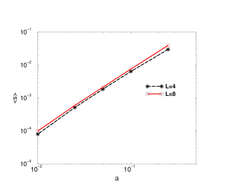
Figure 2: $a$ dependence of the global minima
$\langle s\rangle$ of $V_{eff}$. Horizontal axis is lattice spacing $a$, Vertical one is $\langle s\rangle$. We take here $g_{2}=1$, the solid line is for volume $L=8$, while the dashed line is for $L=4$.

V.3.2 2-point function

We next study whether the contribution from the non-zero momentum mode integral to the 2-point functions are relevant or not in the continuum limit. Among the 2-point terms $(S^{(2)}_{1-loop})^{\alpha_{1}\alpha_{2}}_{\mu\nu}\phi^{\alpha_{1}}_{\mu}\phi^{\alpha_{2}}_{\nu}$ in the Eq. (V.35), the terms of gauge fields are zero due to the gauge symmetry, and only scalar 2-point terms for scalars $s_{x}(=\phi_{0}),s_{y}(=\phi_{2})$ which are $(S^{(2)}_{1-loop})^{\alpha_{1}\alpha_{2}}_{00}\phi^{\alpha_{1}}_{0}\phi^{\alpha_{2}}_{0}$ and $(S^{(2)}_{1-loop})^{\alpha_{1}\alpha_{2}}_{22}\phi_{2}^{\alpha_{1}}\phi^{\alpha_{2}}_{2}$ are only non-zero. They are common due to the $Z_{2}$ symmetry between $x$ and $y$ directions. Their analytical expressions are given in the Appendices. D. In order to study the scaling properties of the ratio $S^{(2)}_{1-loop}/S^{(2)}_{zero}$, it suffices to study $S^{(2)}_{1-loop}$ since the denominator has a fixed value $\frac{\mu}{g_{2}}$ which does not depend on the lattice spacing. The analytic form of $S^{(2)}_{1-loop}$ is

$$(S^{(2)}_{1-loop})^{\alpha_{1}\alpha_{2}}_{\mu\nu} =[ \delta_{\mu,0}\delta_{\nu,0}+\delta_{\mu,2}\delta_{\nu,2}][2\delta^{\alpha_{1},0}\delta^{\alpha_{2},0}S^{(2)}_{1-loop,~{}U(1)}+2M\delta^{\alpha_{1},\alpha_{2}}S^{(2)}_{1-loop,~{}SU(2)}]$$

$$S^{(2)}_{1-loop,~{}U(1)} =\frac{1}{2}[ \frac{1}{N^{2}}\sum_{\mathbf{k}}\frac{2\widehat{\mathbf{k}}^{2}}{(1+\langle s\rangle)^{2}(\widehat{\mathbf{k}}^{2})^{2}}+\frac{(F^{(1)}_{u1}+F^{(2)}_{u1})}{(1+\langle s\rangle)^{2}[\widehat{\mathbf{k}}^{2}(1+\bar{\mu}_{F})+2\bar{\mu}_{F}^{2}]^{2}}$$

$$+\frac{-\frac{1}{2}\widehat{\mathbf{k}}^{2}+\frac{3}{4}\bar{\mu}^{2}}{(1+\langle s\rangle)^{2}(\widehat{\mathbf{k}}^{2}+3\bar{\mu}^{2})-\bar{\mu}^{2}}+\frac{(1+\langle s\rangle)^{2}(\widehat{k_{x}}^{4}+\frac{3}{2}\bar{\mu}^{2}\widehat{\mathbf{k}}^{2}+\frac{9}{2}\bar{\mu}^{4})}{[(1+\langle s\rangle)^{2}(\widehat{\mathbf{k}}^{2}+3\bar{\mu}^{2})-\bar{\mu}^{2}]^{2}}]$$

$$S^{(2)}_{1-loop,~{}SU(2)} =\frac{1}{2}[ \frac{1}{N^{2}}\sum_{\mathbf{k}}\frac{-2\widehat{\mathbf{k}}^{2}}{(1+\langle s\rangle)^{2}(\widehat{\mathbf{k}}^{2})^{2}}+\frac{(F^{(1)}_{su}+F^{(2)}_{su}+F^{(3)}_{su}+F^{(4)}_{su})}{(1+\langle s\rangle)^{2}[\widehat{\mathbf{k}}^{2}(1+\bar{\mu}_{F})+2\bar{\mu}_{F}^{2}]^{2}}$$ (V.37)

$$+\frac{\frac{3}{4}\bar{\mu}^{2}}{(1+\langle s\rangle)^{2}(\widehat{\mathbf{k}}^{2}+3\bar{\mu}^{2})-\bar{\mu}^{2}}+\frac{(1+\langle s\rangle)^{2}(\widehat{k_{x}}^{4}+\frac{3}{2}\bar{\mu}^{2}\widehat{\mathbf{k}}^{2}+\frac{9}{2}\bar{\mu}^{4})}{[(1+\langle s\rangle)^{2}(\widehat{\mathbf{k}}^{2}+3\bar{\mu}^{2})-\bar{\mu}^{2}]^{2}}],$$

where $S^{(2)}_{1-loop,~{}U(1)}$ and $S^{(2)}_{1-loop,~{}SU(2)}$ are the mass correction of the $U(1)$ and $SU(2)$ scalar fields. $F^{(1)}_{u1},F^{(2)}_{u1}$ and $F^{(1)}_{su},F^{(2)}_{su},F^{(3)}_{su},F^{(4)}_{su}$ which appear in the fermion loop contributions to $S^{(2)}_{1-loop,~{}U(1)}$ and $S^{(2)}_{1-loop,~{}SU(2)}$ are given as

$$F^{(1)}_{u1}=-(2\widehat{k_{x}}^{2}(1+\bar{\mu}_{F})+\bar{\mu}_{F}^{2})(1+\bar{\mu}_{F})\quad F^{(2)}_{u1}=-2[(1+\bar{\mu}_{F})^{2}\widehat{k_{y}}^{2}-\bar{\mu}_{F}^{2}](1+\bar{\mu}_{F})\cos(k_{x}a)$$

$$F^{(1)}_{su}=\widehat{k_{x}}^{2}\cos(k_{x}a)[(1+\bar{\mu}_{F})^{2}+1]\quad F^{(2)}_{su}=-\bar{\mu}_{F}(1+\bar{\mu}_{F})^{2}\widehat{k_{x}}^{2}+\bar{\mu}_{F}\widehat{k_{x}}\widehat{3k_{x}}$$

$$F^{(3)}_{su}=\bar{\mu}_{F}^{2}(1+\bar{\mu}_{F})^{2}+\bar{\mu}_{F}\cos(2k_{x}a)\quad F^{(4)}_{su}=[(1+\bar{\mu}_{F})^{2}\widehat{k_{y}}^{2}+\bar{\mu}_{F}^{2}][(1+\bar{\mu}_{F})^{2}+1]$$ (V.38)

In order to see whether the 1-loop correction vanishes in the continuum limit, we evaluate $S^{(2)}_{1-loop,~{}U(1)}$ $S^{(2)}_{1-loop,~{}SU(2)}$ in Eq. (V.37) numerically. The numerical results for several values of ($1/N$, $\bar{\mu}_{F}\equiv r_{F}/N$) with $\bar{\mu}\equiv 1/N$ are given in Figs. 4 and 4, with $r_{F}$ fixed. Figs. 6. 6 shows the results for several values of $r_{F}$ with the lattice spacing $a$ fixed.

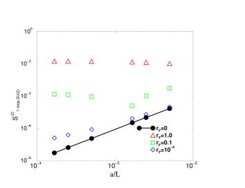
Figure 3: ($1/N$, $\bar{\mu}_{F}=r_{F}/N$) dependence of the nonabelian part of the 1-loop mass correction from the non-zero momentum mode. The horizontal axis is $\frac{1}{N}$ and the vertical axis is $S^{(2)}_{1-loop}$.

.

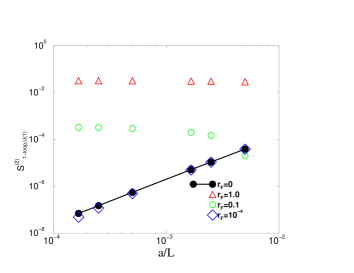
Figure 4: ($1/N$, $\bar{\mu}_{F}=r_{F}/N$) dependence of the abelian part of the 1-loop mass correction from the non-zero momentum mode. The horizontal axis is $\frac{1}{N}$ and the vertical axis is $S^{(2)}_{1-loop}$.

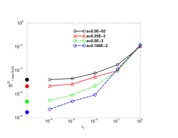
Figure 5: ($1/N$, $\bar{\mu}_{F}=r_{F}/N$) dependence of the nonabelian part of the 1-loop mass correction from the non-zero momentum mode. Horizon axis of this graph is $\frac{\mu_{F}}{\mu}=r_{F}$ and the vertical axis is $S^{(2)}_{1-loop}$. Open symbols denote the data for non-zero $r_{F}$ for fixed lattice spacings. In order to guide the eye, data for the same lattice spacing are connected by straight lines. The filled circles are the values for $r_{F}=0$, for each lattice spacing $a$.

.

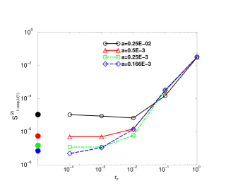
Figure 6: ($1/N$, $\bar{\mu}_{F}=r_{F}/N$) dependence of the abelian part of the 1-loop mass correction from the non-zero momentum mode. Horizon axis of this graph is $\frac{\mu_{F}}{\mu}=r_{F}$ and the vertical axis is $S^{(2)}_{1-loop}$. Open symbols denote the data for non-zero $r_{F}$ for fixed lattice spacings. In order to guide the eye, data for the same lattice spacing are connected by straight lines. The filled circles are the values for $r_{F}=0$, for each lattice spacing $a$.

We find that the 1-loop correction for $r_{F}\neq 0$ does not vanish in the continuum limit, while that for $r_{F}=0$ vanishes. This scaling behavior can be understood as follows. Let us divide the momentum integration region into two parts, i.e. high momentum parts: $\mu\ll p\sim 1/a$, and low momentum parts: $\mu\sim p\ll 1/a$. In high momentum region $\mu$ is a small perturbation and the leading contribution vanishes due to exact susy, while the sub-leading contributions are suppressed by powers in $a$. In low momentum region $\mu$ is not a small perturbation but the integral can be approximated by the continuum expression, e.g. $\sin(p_{\mu}a)\to ap_{\mu}$, $\cos(p_{\mu})\to 1+O((ap)^{2})$ etc. Then the sum can be approximated by the integral with the infra-red cutoff $\bar{k}_{0}\equiv k_{0}a\sim 1/N$ and some intermediate ultra-violet cutoff $\bar{k}_{1}\equiv k_{1}a(\bar{k}_{0}\ll\bar{k}_{1}\ll 1)$:

$$S^{(2)}_{1-loop} \sim 2\delta^{\alpha_{1},0}\delta^{\alpha_{2},0}\displaystyle\int_{\bar{k}_{0}\leq|\bar{\mathbf{k}}|\leq\bar{k}_{1}}\frac{d^{2}\bar{k}}{(2\pi)^{2}}\biggl{[} \frac{2\bar{\mathbf{k}}^{2}}{(\bar{\mathbf{k}}^{2})^{2}}+\frac{-2\bar{\mathbf{k}}^{2}+\bar{\mu}_{F}^{2}}{[\bar{\mathbf{k}}^{2}+2\bar{\mu_{F}}^{2}]^{2}}$$ (V.39)

$$+\frac{-\frac{1}{2}\bar{\mathbf{k}}^{2}+\frac{3}{4}\bar{\mu}^{2}}{\bar{\mathbf{k}}^{2}+2\bar{\mu}^{2}}+\frac{\bar{k}_{x}^{4}+\frac{3}{2}\bar{\mu}^{2}\bar{\mathbf{k}}^{2}+\frac{9}{2}\bar{\mu}^{4})}{[\bar{\mathbf{k}}^{2}+2\bar{\mu}^{2}]^{2}}\biggr{]}$$

$$+2M\delta^{\alpha_{1},\alpha_{2}}\displaystyle\int_{\bar{k}_{0}\leq|\bar{\mathbf{k}}|\leq\bar{k}_{1}}\frac{d^{2}\bar{k}}{(2\pi)^{2}}\biggl{[} \frac{-2\bar{\mathbf{k}}^{2}}{(\bar{\mathbf{k}}^{2})^{2}}+\frac{2\bar{\mathbf{k}}^{2}+\bar{\mu}_{F}+2\bar{\mu}_{F}^{2}}{[\bar{\mathbf{k}}^{2}+2\bar{\mu}_{F}^{2}]^{2}}$$

$$+\frac{\frac{3}{4}\bar{\mu}^{2}}{\bar{\mathbf{k}}^{2}+2\bar{\mu}^{2}}+\frac{\bar{k}_{x}^{4}+\frac{3}{2}\bar{\mu}^{2}\bar{\mathbf{k}}^{2}+\frac{9}{2}\bar{\mu}^{4}}{[\bar{\mathbf{k}}^{2}+2\bar{\mu}^{2}]^{2}}\biggr{]},$$

where we have set $\langle s\rangle=0$ for simplicity. Then the first two terms in each integration give rise to contributions linear and logarithmic in the infra-red cutoff as

$$S^{(2)}_{1-loop} \sim 2\delta^{a_{1},0}\delta^{a_{2},0}\biggl{[} \frac{1}{4\pi}(2log(\frac{\bar{k}_{1}^{2}}{\bar{k}_{0}^{2}})-2log(\frac{\bar{k}_{1}^{2}+2\bar{\mu}_{F}^{2}}{\bar{k}_{0}^{2}+2\bar{\mu}_{F}^{2}})+\frac{5\bar{\mu}_{F}^{2}}{\bar{k}_{0}^{2}+2\bar{\mu}_{F}^{2}})\biggr{]}$$ (V.40)

$$+2M\delta^{a_{1},a_{2}}\biggl{[} \frac{1}{4\pi}(-2log(\frac{\bar{k}_{1}^{2}}{\bar{k}_{0}^{2}})+2log(\frac{\bar{k}_{1}^{2}+2\bar{\mu}_{F}^{2}}{\bar{k}_{0}^{2}+2\bar{\mu}_{F}^{2}})+\frac{\bar{\mu}_{F}-2\bar{\mu}_{F}^{2}}{\bar{k}_{0}^{2}+2\bar{\mu}_{F}^{2}})\biggr{]}.$$

which give volume independent mass terms in the continuum limit. One might naively wonder why setting $\mu=\mu_{F}$ and taking the limits (1) $a\to 0$ then (2) $1/L\to 0$ does not work. This is because the contributions from infra-red parts are not completely canceled out due to the asymmetry between the infra-red regulator of boson and fermion as mentioned in Sec. III, although the contributions from the UV part are canceled as expected.

In order to avoid the appearance of such counter terms, one should adopt the following procedure:

1. Compute physical quantities for fixed ($1/N$, $\bar{\mu}_{F}=r_{F}/N$).

2. Take $\mu_{F}\to 0$ with fixed $1/N$ first , i.e $r_{F}\to 0$.

3. Then take the continuum limit, i.e. $1/N\to 0$ .

This two-step limit can avoid the counter terms as can be seen from Eq. (V.40).

V.4 Procedure 4: non-perturbative study of the zero momentum mode

From the results of procedure 3 in the previous section, no term of 1-loop contributions from non-zero momentum modes to the effective action in Eq. (V.35) can survive in the continuum limit. Therefore in order to evaluate 1- and 2-point functions in the continuum limit, we only have to perform the following integral

$$I_{n}^{\alpha_{1}\cdots\alpha_{n}}=L^{\frac{3n}{2}}g_{2}^{\frac{n}{2}}\frac{\int d\tilde{\phi}(\mathbf{0})det[D_{\psi}(\mathbf{0})]\displaystyle{\prod_{i=1}^{n}}(\tilde{s}^{\alpha_{i}}_{\mu}(0))e^{-S_{fin}}}{\int d\tilde{\phi}(\mathbf{0})det[D_{\psi}(\mathbf{0})]e^{-S_{fin}}},$$ (V.41)

$$S_{fin}=\sum_{\mu>\nu}Tr[\tilde{\phi}_{\mu}(0),\tilde{\phi}_{\nu}(0)]^{2}+\frac{\mu}{g_{2}}Tr[(\tilde{s}_{x}(0)^{2}+\tilde{s}_{y}(0)^{2})].$$ (V.42)

We discuss whether the fine-tuning is needed or not by the investigation of the infinite volume behavior of this value.

To calculate Eq. (V.41), we should first express the fermion determinant $det[D_{\psi}(\mathbf{0})]$ from the zero momentum modes as the function of bosonic fields analytically. In the integral with only zero momentum bosonic modes, we can ignore the coordinate indices $\mathbf{n}$, As is obvious from Eq. (V.32) the fermion determinant $det[D_{\psi}(\mathbf{0})]$ is given as

$$det[D_{\psi}(\mathbf{0})] =\bar{\mu}_{F}^{2}det\left(\begin{array}[]{c|c|c}\bar{\mu}_{F}E^{\prime}_{2,2}+\left(\frac{\bar{g}}{N}\right)^{\frac{1}{2}}E_{(2,2)\mathbf{0},\mathbf{0}}^{ab}&\left(\frac{\bar{g}}{N}\right)^{\frac{1}{2}}\bar{\mu}_{F}F_{\xi(2,1)\mathbf{0},\mathbf{0}}^{a0}&\left(\frac{\bar{g}}{N}\right)^{\frac{1}{2}}\bar{\mu}_{F}F_{\lambda(2,1)\mathbf{0},\mathbf{0}}^{a0}\\ \hline\cr\left(\frac{\bar{g}}{N}\right)^{\frac{1}{2}}H_{\lambda(2,1)\mathbf{0},\mathbf{0}}^{0b}&1&-1\\ \hline\cr\left(\frac{\bar{g}}{N}\right)^{\frac{1}{2}}K_{(1,2)\mathbf{0},\mathbf{0}}^{0b}&1&1\end{array}\right).$$ (V.46)

If one takes $\mu_{F}\to 0$ limit as the first part of the two step limit, which was explained in Sec. V.3 the determinant is simplified to a determinant of the $SU(2)$ group

$$det[D_{\psi}(\mathbf{0})]\sim 2\left(\frac{\bar{g}}{N}\right)^{\frac{1}{2}}\bar{\mu}_{F}^{2}det(E_{(2,2)\mathbf{0},\mathbf{0}}^{ab}),$$ (V.48)

which is the fermion determinant of the following $SU(2)$ matrix model.

$$S=Tr(\frac{1}{2}\sum_{\mu>\nu}[\tilde{\phi}_{\mu},\tilde{\phi}_{\nu}]^{2}+\bar{\psi}\gamma_{\mu}[\tilde{\phi}_{\mu},\psi]),$$ (V.49)

where

$$\tilde{\phi}_{\mu}=\tilde{\phi}_{\mu}^{a}T^{a},(\mu=0,1,2,3)$$ (V.50)

$$\tilde{\phi}_{0}^{a}=\tilde{s}_{x}^{a},\,\tilde{\phi}_{1}^{a}=-\tilde{v}_{y}^{a},\,\tilde{\phi}_{2}^{a}=\tilde{s}_{y}^{a},\,\tilde{\phi}_{3}^{a}=-\tilde{v}_{x}^{a}.$$ (V.51)

with $T^{a}$s being $SU(2)$ generators. This action is invariant under $SO(4)$ Lorentz transformation

$$\tilde{\phi}_{\mu}\to\Lambda^{\nu}_{\mu}\tilde{\phi}_{\nu},$$ (V.52)

where $(\Lambda)^{\mu}_{\nu}$ is the $SO(4)$ matrix.

The explicit form of the fermion determinant $det[D_{\psi}(\mathbf{0})]$ is

$$det[D_{\psi}(\mathbf{0})]= \frac{1}{\bar{g}^{12}}[(\tilde{\phi}^{1}\cdot\tilde{\phi}^{1})(\tilde{\phi}^{2}\cdot\tilde{\phi}^{2})(\tilde{\phi}^{3}\cdot\tilde{\phi}^{3})$$

$$-(\tilde{\phi}^{1}\cdot\tilde{\phi}^{1})(\tilde{\phi}^{2}\cdot\tilde{\phi}^{3})^{2}-(\tilde{\phi}^{2}\cdot\tilde{\phi}^{2})(\tilde{\phi}^{1}\cdot\tilde{\phi}^{3})^{2}-(\tilde{\phi}^{3}\cdot\tilde{\phi}^{3})(\tilde{\phi}^{1}\cdot\tilde{\phi}^{2})^{2}$$

$$+2(\tilde{\phi}^{1}\cdot\tilde{\phi}^{2})(\tilde{\phi}^{2}\cdot\tilde{\phi}^{3})(\tilde{\phi}^{3}\cdot\tilde{\phi}^{1})]=\frac{1}{\bar{g}^{12}}det(\tilde{\phi}^{a}\cdot\tilde{\phi}^{b}),$$ (V.53)

$$(\tilde{\phi}^{a}\cdot\tilde{\phi}^{b}\equiv\sum_{\mu=0}^{3}\tilde{\phi}^{a}_{\mu}\tilde{\phi}^{b}_{\mu}),$$ (V.54)

which can be obtained as in Ref. Suyama-Tsuchiya .

From (V.42) and (V.53), one can see that the fermion determinant and the bosonic action are even functions in $\tilde{\phi}_{\mu}$. Since the 1-point function is odd in $\tilde{\phi}_{\mu}$, the integration of numerator of Eq. (V.41) for $n=1$ case trivially vanishes.

We now carry out the integral over the bosonic zero momentum mode in Eq. (V.41) for 2-point function non-perturbatively. We can decompose the action $S_{fin}$ as $S_{fin}=S_{SU(2)}+S_{U(1)}$, where $S_{SU(2)}$ and $S_{U(1)}$ are the actions for the $SU(2)$ and $U(1)$ part as

$$S_{SU(2)}=\sum_{\mu>\nu}Tr[\tilde{\phi}_{\mu}(0),\tilde{\phi}_{\nu}(0)]^{2},+\frac{\mu}{g_{2}}[(\tilde{s}^{a}_{x}(0))^{2}+(\tilde{s}^{a}_{y}(0))^{2}],$$ (V.55)

$$S_{U(1)}=\frac{\mu}{g_{2}}[(\tilde{s}^{0}_{x}(0))^{2}+(\tilde{s}^{0}_{y}(0))^{2}].$$ (V.56)

Thus the 2-point function in Eq. (V.41) can be factorized into the product of integrals over $U(1)$ fields and $SU(2)$ fields. Since the fermion determinant is independent of the $U(1)$ part of the scalar fields, the $U(1)$ part of the 2-point function $I_{2}^{0,0}$ becomes a trivial gaussian integral and is identical to the tree level value $g_{2}L^{4}$. Therefore only the $SU(2)$ part of the 2-point function $I_{2}^{a,b}$ becomes nontrivial as

$$I^{a,b}_{2}=g_{2}L^{3}\frac{\int d\tilde{s}_{x}^{a}(\mathbf{0})d\tilde{v}_{x}^{a}(\mathbf{0})d\tilde{s}_{y}^{a}(\mathbf{0})d\tilde{s}_{y}^{a}(\mathbf{0})(\tilde{s}_{\mu}(0))^{a}(\tilde{s}_{\mu}(0))^{b}det[D_{\psi}(\mathbf{0})]e^{-S_{SU(2)}}}{\int d\tilde{s}_{x}^{a}(\mathbf{0})d\tilde{v}_{x}^{a}(\mathbf{0})d\tilde{s}_{y}^{a}(\mathbf{0})d\tilde{s}_{y}^{a}(\mathbf{0})det[D_{\psi}(\mathbf{0})]e^{-S_{SU(2)}}}\equiv\delta^{a,b}\langle ss\rangle.$$ (V.57)

Since $\langle ss\rangle$ is the zero momentum mode of the propagator, it can be written by the renormalized mass squared $m_{R}^{2}$ which is the sum of the tree level mass squared $\frac{\mu^{2}}{g_{2}^{2}}$ and the quantum correction $\Delta\mu^{2}$.

$$\frac{1}{L^{2}}\langle ss\rangle=\frac{1}{m_{R}^{2}}=\frac{1}{\frac{\mu^{2}}{g_{2}^{2}}+\Delta\mu^{2}}\quad$$ (V.58)

If there is no quantum correction, the 2-point function becomes the tree level value $\langle ss\rangle_{tree}$ with $L$ dependence

$$\frac{1}{L^{2}}\langle ss\rangle_{tree}=\left(\frac{\mu^{2}}{g_{2}^{2}}\right)^{-1}=g_{2}L^{2}.$$ (V.59)

V.4.1 Numerical calculation of the 2-point function

We perform the integral in Eq. (V.57) numerically. Simulations are carried out in the Metropolis algorithm with $2.0\times 10^{5}$ sweeps for the thermalization and $2.0\times 10^{7}$ sweeps for the measurement. We estimate the error by the variance with binsize of $100$ sweeps.

Since the 2-point function depends only on the product $g_{2}L$, we take $g_{2}=1$ without loosing generality. Fig. 7 shows the $L$ dependence of the 2-point function $\langle ss\rangle$.

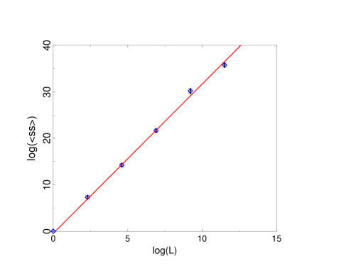
Figure 7: The lattice size $L$ dependence of the 2-point function. The horizontal axis is $L$, where as the vertical axis is $\langle ss\rangle$.

As can be seen in Fig. 7, we find that $\langle ss\rangle$ increases with $L$. Fitting the data with the following function

$$\langle ss\rangle\sim AL^{3+\alpha},$$ (V.60)

we obtain $A=0.65(20)$ and $\alpha=0.210(46)$. This gives the $L$ dependence of the renormalized mass

$$m_{R}^{2}\equiv\frac{\mu^{2}}{g_{2}^{2}}+\Delta\mu^{2}\equiv L^{2}\langle ss\rangle^{-1}\sim\frac{1}{AL^{1+\alpha}},$$ (V.61)

which vanishes in the large volume limit $L\to\infty$. Our result also implies that the contribution from the quantum corrections becomes dominant for large $L$. Thus in the continuum limit for finite volume, there is a non-trivial mass correction which is larger than the tree level contribution $\frac{\mu}{g_{2}}$. However, after taking the infinite volume limit the mass term vanishes so that there is no need for fine-tuning.

VI Constraint from the stability of the lattice spacetime

In this section we study the stability of the lattice spacetime by the deconstruction against quantum effects. In Sec. V.3.1, we found that with sufficiently small $\bar{g}$ and fixed $L$, there is a minimum of the 1-loop potential $V(\langle s\rangle)$ near the tree-level value and that the 1-loop shift of the expectation value vanishes towards the continuum limit so that the quantum correction becomes irrelevant. However, this may not always be the case for any choices of the parameters. In general the tree level contribution of the potential is proportional to $\frac{\mu}{g_{2}}\sim\frac{1}{g_{2}L}$, whereas the 1-loop correction depends on $\bar{\mu}$. If $g_{2}L$ is too large there is a possibility that global minima may disappear and the lattice spacetime structure can be destroyed due to large quantum effects. Therefore it is quite important to investigate in the parameter region of interest where the physical correlation length $g_{2}^{-1}$ is larger than the lattice spacing $a$ but smaller lattice size $L$,

$$a\ll(g_{2})^{-1}\ll L,$$ (VI.1)

In Fig. 9, we show the effective potential for $N=400$ and $\bar{g}_{2}=0.075$. We find that there is no minimum of the potential at 1-loop level. Fig. 9 shows the 1-loop potential with the same $\bar{g}=g_{2}a$ but smaller volume $N=200$, where we find that there is a minimum. From this fact it becomes clear that we cannot take too large volume in the region where $\bar{g}$ is not so small.

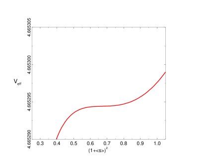
Figure 8: The graph of $\langle s\rangle$dependence of $V_{eff}$ for $N=400,\bar{g}^{2}=0.075\gtrsim 0.2$.
The horizontal axis is $(1+\langle s\rangle)^{2}$, while the vertical axis is $V_{eff}$.

.

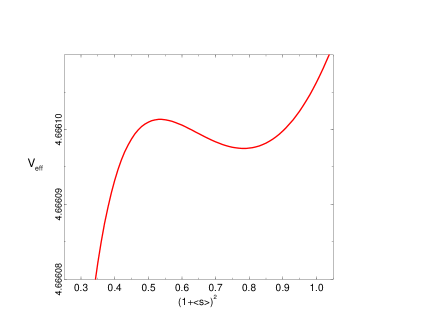
Figure 9: The graph of $\langle s\rangle$dependence of $V_{eff}$ for $N=200,\bar{g}^{2}=0.075\gtrsim 0.2$.
The horizontal axis is $(1+\langle s\rangle)^{2}$, while the vertical axis is $V_{eff}$.

The above observation suggests that the set of parameters ($\bar{g}=g_{2}a$, $N=L/a$) or equivalently ($\bar{g}=g_{2}a$, $g_{2}L$) has to satisfy some constraints in order to stabilize the vacuum with a spacetime structure. Fig. 10 shows the constraints on the parameter region for ($\bar{g}=g_{2}a$, $g_{2}L$) where the deconstructed spacetime can be stabilized. We have set $g_{2}=1$ without loosing generality. Lattice spacing $a$ in this graph can be regarded as the strength of couplings $\bar{g}$. In Fig. 10, the parameter region with stable spacetime structure is denoted by the symbol ’$\times$’ whereas those with no stable spacetime structure is denoted by the symbol ’$+$’. It is clear that taking the continuum limit before taking the large volume limit has a crucial role to stabilize the lattice structure.

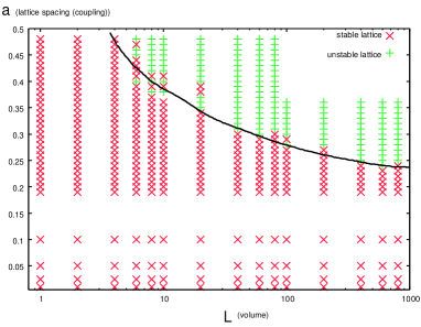
Figure 10: The constraints on the parameter region of ($\bar{g}=g_{2}a=a,g_{2}L=L$) for the stability of the deconstructed spacetime. The symbols $\times$ show the region where the spacetime is stabilized, while the symbols $+$ show the region where the spacetime is not stabilized.

VI.1 Role of the supersymmetry for Deconstruction

In the discussion of Sec. V.3.1, it seems that cancellation of 1-loop effect between fermion and boson is crucial for stabilizing the ’Deconstruction’ vacuum. In order to see the role of the supersymmetry, we now study the bosonic model where the fermions are dropped from the theory.

The 1-loop effective potential for the bosonic model is

$$V_{eff}(\langle s\rangle)= \frac{\bar{\mu}^{2}}{2\bar{g}^{2}}[(1+\langle s\rangle)^{2}-1]^{2}M$$

$$+\sum_{\mathbf{k}}\frac{1}{N^{2}}log[(1+\langle s\rangle)^{2}(\widehat{\mathbf{k}}^{2}+3\bar{\mu}^{2})-\bar{\mu}^{2}]M^{2}$$ (VI.2)

We have to check whether this potential (VI.2) have stationary point or not. The stationary point of this potential $\langle s\rangle_{b}$ must satisfy following equation.

$$0 =\frac{d}{d\langle s\rangle}V_{eff}(\langle s\rangle_{b})$$

$$=\frac{\bar{\mu}^{2}}{\bar{g}^{2}}(1+\langle s\rangle_{b})((1+\langle s\rangle_{b})^{2}-1)M$$

$$+\frac{1}{N^{2}}\sum_{\mathbf{k}}\frac{2(1+\langle s\rangle_{b})(\hat{\mathbf{k}}^{2}+3\bar{\mu}^{2})}{(1+\langle s\rangle_{b})^{2}\hat{\mathbf{k}}^{2}+(3(1+\langle s\rangle_{b})^{2}-1)\bar{\mu}^{2}}M^{2}.$$ (VI.3)

In order to have a well-defined perturbative vacuum with no tachyons $\frac{1}{3}<(1+\langle s\rangle)^{2}$ has to be satisfied. In this region the second term in Eq. (VI.3) is positive. Therefore, the minimum can only exist in the region $(1+\langle s\rangle)^{2}<1$, since otherwise the first term in Eq. (VI.3) is also positive. Now when $\frac{1}{3}<(1+\langle s\rangle)^{2}<1$, the second term is larger than $M^{2}$, and first term is larger than $-\frac{\bar{\mu}^{2}}{\bar{g}^{2}}M$ so that

$$\frac{d}{d\langle s\rangle}V_{eff}>M^{2}-\frac{\bar{\mu}^{2}}{\bar{g}^{2}}M.$$ (VI.4)

Since $M>1$ for non-abelian gauge group,

$$\frac{d}{d\langle s\rangle}V_{eff}>0, \frac{\bar{\mu}}{\bar{g}}=(g_{2}L)^{-1}<1,$$ when (VI.5)

so that there is no stable minimum near the tree level minimum in all the physically natural parameter region as given in Eq. (VI.1). Although it is difficult to find the global minimum with large order correction in perturbation theory, Eq. (VI.5) suggests that the quantum effect in the bosonic model has the effect to drive VEV $(1+\langle s\rangle)/\sqrt{2}a$ to smaller value, which corresponds to larger lattice spacing. Eq. (VI.5) imply that the deconstruction cannot make a stable spacetime if there is no fermion-boson cancellation. The instability of the bosonic model was also observed by Giedt Giedt 0312 in his non-perturbative study on the bosonic part of the CKKU model for the (4,4) 2d super-Yang-Mills Kaplan3 where he found that the bosonic fields $x$ seem to concentrate at $\langle x\rangle\sim 0$. From these observation one can say the CKKU model has a stable vacuum not simply because the quantum correction is small but because the quantum corrections from the fermionic modes and bosonic modes cancel, which means that the supersymmetry is crucial for the stabilization of the deconstruction.

VI.2 The meaning of 1-loop calculation for the study of stabilization of lattice spacing

We calculated the 1-loop effective potential using the Coleman-Weinberg method. In order to study the stability of the theory, of course one has to carry out non-perturbative analyses eventually. However, it would be still useful to study the effective potential in 1-loop approximation for two reasons; (1) By obtaining analytical forms of the potential or correlation functions at 1-loop, one can understand the detailed structure of quantum corrections. (2) The perturbative result would also be useful for future non-perturbative numerical calculations, since it gives us a quantitative idea on the appropriate parameter region in which the simulation should be carried out with good stability of the vacuum and scaling property.

VII Conclusion and discussion

In this paper, we have studied the CKKU model at the quantum level by an explicit perturbative calculation for the case of $U(2)$ gauge group. We have pointed the subtleties of the perturbative correction in CKKU model which arises from the zero-eigenvalue of the fermion-matrix and the massless zero momentum mode of the bosonic fields. To make the fermion path-integral well-defined, we have introduced the fermion mass term in Eq. (III.4), although we have find that the two-step limit, where we take the limit of zero fermion mass at first before taking the continuum limit, is necessary to control the counter terms. In order to avoid the infra-red divergences we have separated the zero momentum modes and carried out the path-integral over these fields non-perturbatively, while non-zero momentum modes are treated perturbatively.

We have then studied the possible counter terms in this model, namely the bosonic 1-point and 2-point functions by the explicit calculation. We have found that there are non-trivial quantum mass corrections larger than the tree level mass. However these corrections vanish in the infinite volume limit so that the CKKU model does not need fine-tuning to recover the full supersymmetry.

We have also studied the stability of the lattice spacetime generated by the ‘deconstruction’. We have found the constraint on the parameter region for which the lattice spacetime is stable against 1-loop corrections. This constraint is not only interesting quantitative information of the property of the lattice spacetime, but also practically useful as a guide for the fully numerical non-perturbative simulations in the future. We have also understood that the cancellation of quantum corrections between bosons and fermions is crucial to stabilize the lattice spacetime.

It would of course be important to make a full non-perturbative study of CKKU model in our prescription. In particular, a comparison of the result with the study by Giedt Giedt 0405 by a phase quenched model would be interesting. Recently, there are new lattice theories which preserve the supersymmetry on the lattice Catterall:2001wx -Kanamori2 . These are the models without deconstruction, and might be useful for the practical study. The perturbative study of these models would also be important.

Appendix A Notation and fourier transformation

Now we define the fourier transformation of the fields on the lattice as follows.

$$\tilde{s}_{x}(\mathbf{0})=a\frac{1}{\sqrt{\bar{g}N^{3}}}\sum_{\mathbf{n}}s_{x\mathbf{n}}\quad\tilde{v}_{x}(\mathbf{0})=\sum_{\mathbf{n}}a\frac{1}{\sqrt{\bar{g}N^{3}}}v_{x\mathbf{n}}$$ (A.1)

$$\tilde{s}_{y}(\mathbf{0})=\sum_{\mathbf{n}}a\frac{1}{\sqrt{\bar{g}N^{3}}}s_{y\mathbf{n}}\quad\tilde{v}_{y}(\mathbf{0})=\sum_{\mathbf{n}}a\frac{1}{\sqrt{\bar{g}N^{3}}}v_{y\mathbf{n}}$$ (A.2)

$$\tilde{s}_{x}(\mathbf{k}\neq\mathbf{0})=a\frac{1}{\bar{g}N}\sum_{\mathbf{n}}s_{x\mathbf{n}}e^{-ia\mathbf{k}\cdot\mathbf{n}}e^{-ia\frac{1}{2}k_{x}}\quad\tilde{v}_{x}(\mathbf{k}\neq\mathbf{0})=\sum_{\mathbf{n}}a\frac{1}{\bar{g}N}v_{x\mathbf{n}}e^{-ia\mathbf{k}\cdot\mathbf{n}}e^{-ia\frac{1}{2}k_{x}}$$ (A.3)

$$\tilde{s}_{y}(\mathbf{k}\neq\mathbf{0})=\sum_{\mathbf{n}}a\frac{1}{\bar{g}N}s_{y\mathbf{n}}e^{-ia\mathbf{k}\cdot\mathbf{n}}e^{-ia\frac{1}{2}k_{y}}\quad\tilde{v}_{y}(\mathbf{k}\neq\mathbf{0})=\sum_{\mathbf{n}}a\frac{1}{\bar{g}N}v_{y\mathbf{n}}e^{-ia\mathbf{k}\cdot\mathbf{n}}e^{-ia\frac{1}{2}k_{y}}$$ (A.4)

$$\hat{x}_{\mathbf{0}}=a\frac{1}{\sqrt{\bar{g}N^{3}}}\sum_{\mathbf{n}}(x_{\mathbf{n}}-\frac{1}{\sqrt{2}a})\quad\hat{\bar{x}}_{\mathbf{0}}=a\frac{1}{\sqrt{\bar{g}N^{3}}}\sum_{\mathbf{n}}(\bar{x}_{\mathbf{n}}-\frac{1}{\sqrt{2}a})$$

$$\hat{y}_{\mathbf{0}}=a\frac{1}{\sqrt{\bar{g}N^{3}}}\sum_{\mathbf{n}}(y_{\mathbf{n}}-\frac{1}{\sqrt{2}a})\quad\hat{\bar{y}}_{\mathbf{0}}=a\frac{1}{\sqrt{\bar{g}N^{3}}}\sum_{\mathbf{n}}(\bar{y}_{\mathbf{n}}-\frac{1}{\sqrt{2}a})$$ (A.5)

$$\hat{x}_{\mathbf{k}\neq 0}=a\frac{1}{\bar{g}N}\sum_{\mathbf{n}}(x_{\mathbf{n}}-\frac{1}{\sqrt{2}a})e^{-ia\mathbf{k}\cdot\mathbf{n}}\quad\hat{\bar{x}}_{\mathbf{k}\neq 0}=a\frac{1}{\bar{g}N}\sum_{\mathbf{n}}(\bar{x}_{\mathbf{n}}-\frac{1}{\sqrt{2}a})e^{-ia\mathbf{k}\cdot\mathbf{n}}$$

$$\hat{y}_{\mathbf{k}\neq 0}=a\frac{1}{\bar{g}N}\sum_{\mathbf{n}}(y_{\mathbf{n}}-\frac{1}{\sqrt{2}a})e^{-ia\mathbf{k}\cdot\mathbf{n}}\quad\hat{\bar{y}}_{\mathbf{k}\neq 0}=a\frac{1}{\bar{g}N}\sum_{\mathbf{n}}(\bar{y}_{\mathbf{n}}-\frac{1}{\sqrt{2}a})e^{-ia\mathbf{k}\cdot\mathbf{n}}$$ (A.6)

$$\tilde{\alpha}_{\mathbf{0}}=a^{\frac{3}{2}}\frac{1}{\sqrt{\bar{g}N^{3}}}\sum_{\mathbf{n}}\alpha_{\mathbf{n}}e^{-ia\mathbf{k}\cdot\mathbf{n}}e^{-ia\frac{1}{2}k_{x}}\quad\tilde{\beta}_{\mathbf{0}}=a^{\frac{3}{2}}\frac{1}{\sqrt{\bar{g}N^{3}}}\sum_{\mathbf{n}}\beta_{\mathbf{n}}e^{-ia\mathbf{k}\cdot\mathbf{n}}e^{-ia\frac{1}{2}k_{y}}$$ (A.7)

$$\tilde{\lambda}_{\mathbf{0}}=a^{\frac{3}{2}}\frac{1}{\sqrt{\bar{g}N^{3}}}\sum_{\mathbf{n}}\lambda_{\mathbf{n}}e^{-ia\mathbf{k}\cdot\mathbf{n}}\quad\tilde{\xi}_{\mathbf{0}}=a^{\frac{3}{2}}\frac{1}{\sqrt{\bar{g}N^{3}}}\sum_{\mathbf{n}}\xi_{\mathbf{n}}e^{-ia\mathbf{k}\cdot\mathbf{n}}e^{-ia\frac{1}{2}(k_{x}+k_{y})}$$ (A.8)

$$\tilde{\alpha}_{\mathbf{k}\neq\mathbf{0}}=a^{\frac{3}{2}}\frac{1}{\bar{g}N}\sum_{\mathbf{n}}\alpha_{\mathbf{n}}e^{-ia\mathbf{k}\cdot\mathbf{n}}e^{-ia\frac{1}{2}k_{x}}\quad\tilde{\beta}_{\mathbf{k}\neq\mathbf{0}}=a^{\frac{3}{2}}\frac{1}{\bar{g}N}\sum_{\mathbf{n}}\beta_{\mathbf{n}}e^{-ia\mathbf{k}\cdot\mathbf{n}}e^{-ia\frac{1}{2}k_{y}}$$ (A.9)

$$\tilde{\lambda}_{\mathbf{k}\neq\mathbf{0}}=a^{\frac{3}{2}}\frac{1}{\bar{g}N}\sum_{\mathbf{n}}\lambda_{\mathbf{n}}e^{-ia\mathbf{k}\cdot\mathbf{n}}\quad\tilde{\xi}_{\mathbf{k}\neq\mathbf{0}}=a^{\frac{3}{2}}\frac{1}{\bar{g}N}\sum_{\mathbf{n}}\xi_{\mathbf{n}}e^{-ia\mathbf{k}\cdot\mathbf{n}}e^{-ia\frac{1}{2}(k_{x}+k_{y})}$$ (A.10)

We denote two-dimensional momentum as $\mathbf{k}\equiv(k_{x},k_{y})$. And we define the lattice momentum $\widehat{k_{x,y}},\widehat{\mathbf{k}}$ as

$$\widehat{k^{\prime}_{x}}=\frac{2}{a}\sin(\frac{ak_{x}}{2}),\quad\widehat{k_{x}}=a\widehat{k^{\prime}_{x}}=2\sin(\frac{ak_{x}}{2})$$ (A.11)

$$\widehat{k^{\prime}_{y}}=\frac{2}{a}\sin(\frac{ak_{y}}{2}),\quad\widehat{k_{y}}=a\widehat{k^{\prime}_{y}}=2\sin(\frac{ak_{y}}{2})$$ (A.12)

$$\widehat{\mathbf{k}}^{2}\equiv\widehat{k_{x}}^{2}+\widehat{k_{y}}^{2}\quad$$ (A.13)

The coupling $\bar{g}$, and the masses $\bar{\mu},\bar{\mu_{F}}$ in the lattice unit are defined as

$$\bar{g}=g_{2}a,\bar{\mu}=a\mu=\frac{1}{N},\bar{\mu_{F}}=a\mu_{F}$$ (A.14)

We denote generators of gauge group $U(2)$ with fundamental representation as $2\times 2$ matrices $T^{\mu},(\mu=0,1,2,3)$ ,where $T^{0}$ is the one of $U(1)\subset U(2)$ and $T^{1},T^{2},T^{3}$ are ones for $SU(2)\subset U(2)$.

We also define $t^{\mu\nu\rho}$ and $t^{\mu\nu\rho}_{\mathbf{m},\mathbf{n}}$ as

$$t^{\mu\nu\rho}_{\mathbf{m},\mathbf{n}}\equiv t^{\mu\nu\rho}\delta_{\mathbf{m},\mathbf{n}}\equiv\frac{1}{2}Tr(T^{\mu}T^{\nu}T^{\rho})\delta_{\mathbf{m},\mathbf{n}}.$$ (A.15)

Appendix B fermion matrix

Momentum representation of fermion action is written as

$$\bar{g}^{-2}N^{2}\Bigl{(}\begin{array}[]{cc|cc|c|c}\tilde{\alpha}_{\mathbf{k}}^{\mu},&\tilde{\beta}_{\mathbf{k}}^{\mu},&\tilde{\alpha}_{\mathbf{0}}^{a(\neq 0)},&\tilde{\beta}_{\mathbf{0}}^{a(\neq 0)},&\tilde{\beta}_{\mathbf{0}}^{0},&\tilde{\alpha}_{\mathbf{0}}^{0}\end{array}\Bigr{)}\cdot$$ (B.2)

$$\left(\begin{array}[]{c|c|c|c}\bar{g}^{2}\bar{A}_{(2,2)\mathbf{k},\mathbf{p}}^{\mu\nu}&\bar{g}^{\frac{5}{2}}B_{(2,2)\mathbf{k},\mathbf{0}}^{\mu b}&\bar{g}^{\frac{5}{2}}C_{\xi(2,1)\mathbf{k},\mathbf{0}}^{\mu 0}&\bar{g}^{\frac{5}{2}}\bar{\mu}_{F}C_{\lambda(2,1)\mathbf{k},\mathbf{0}}^{\mu 0}\\ \hline\cr\bar{g}^{\frac{5}{2}}D_{(2,2)\mathbf{0},\mathbf{p}}^{a\nu}&\bar{g}\bar{\mu}_{F}E^{\prime}_{2,2}+\bar{g}^{\frac{3}{2}}E_{(2,2)\mathbf{0},\mathbf{0}}^{ab}&\bar{g}^{\frac{3}{2}}\bar{\mu}_{F}F_{\xi(2,1)\mathbf{0},\mathbf{0}}^{a0}&\bar{g}^{\frac{3}{2}}\bar{\mu}_{F}F_{\lambda(2,1)\mathbf{0},\mathbf{0}}^{a0}\\ \hline\cr\bar{g}^{\frac{5}{2}}G_{(1,2)\mathbf{0},\mathbf{p}}^{0\nu}&\bar{g}^{\frac{3}{2}}\bar{\mu}_{F}H_{\lambda(2,1)\mathbf{0},\mathbf{0}}^{0b}&\bar{g}\bar{\mu}_{F}&-\bar{g}\bar{\mu}_{F}\\ \hline\cr\bar{g}^{\frac{5}{2}}J_{(1,2)\mathbf{0},\mathbf{p}}^{0\nu}&\bar{g}^{\frac{3}{2}}\bar{\mu}_{F}K_{(1,2)\mathbf{0},\mathbf{0}}^{0b}&\bar{g}\bar{\mu}_{F}&\bar{g}\bar{\mu}_{F}\end{array}\right)\left(\begin{array}[]{c}\tilde{\lambda}_{\mathbf{p}}^{\nu}\\ \tilde{\xi}_{\mathbf{p}}^{\nu}\\ \hline\cr\tilde{\lambda}_{\mathbf{0}}^{a(\neq 0)}\\ \tilde{\xi}_{\mathbf{0}}^{a(\neq 0)}\\ \hline\cr\tilde{\xi}_{\mathbf{0}}^{0}\\ \hline\cr\tilde{\lambda}_{\mathbf{0}}^{0}\end{array}\right),$$ (B.13)

where the sub-matrices $\bar{A}_{(2,2)\mathbf{k},\mathbf{p}}^{\mu\nu},B_{(2,2)\mathbf{k},\mathbf{0}}^{\mu b},\cdots,K_{(1,2)\mathbf{0},\mathbf{0}}^{0b}$ are of order unity with respect to $\bar{\mu}$,$\bar{\mu}_{F}$ and $\bar{g}$. In this section, we take generators with subscripts written in Roman letters $a,b$ as the generators of $SU(2)\subset U(2)$, and ones with subscripts written in Greek characters $\mu,\nu$ as generators of $U(2)$. The explicit forms of sub-matrices of fermion matrix are given as follows:

$$\bar{A}_{(2,2)\mathbf{k},\mathbf{p}}^{\mu\nu}=\left(\begin{array}[]{cc}a_{1,1}&a_{1,2}\\ a_{2,1}&a_{2,2}\end{array}\right),$$ (B.16)

where

$$a_{1,1}= (i\widehat{k_{x}}+\bar{\mu}_{F}e^{(\frac{iak_{x}}{2})})(1+\langle s\rangle)\delta_{\mathbf{k}+\mathbf{p},\mathbf{0}}\delta^{\mu\nu}$$

$$+(\bar{g}\hat{\bar{x}}_{\mathbf{q}\neq\mathbf{0}}+\bar{g}^{\frac{1}{2}}\hat{\bar{x}}_{\mathbf{q}=\mathbf{0}})^{\rho}(t^{\mu\rho\nu}e^{(\frac{-ip_{x}}{2})}(1+\bar{\mu}_{F})-t^{\mu\nu\rho}e^{(\frac{ip_{x}}{2})})\delta_{\mathbf{k}+\mathbf{p}+\mathbf{q},\mathbf{0}},$$ (B.17)

$$a_{1,2}= (i\widehat{k_{y}}-\bar{\mu}_{F}e^{(\frac{-iak_{y}}{2})})(1+\langle s\rangle)\delta_{\mathbf{k}+\mathbf{p},\mathbf{0}}\delta^{\mu\nu}$$

$$+(\bar{g}\hat{y}_{\mathbf{q}\neq\mathbf{0}}+\bar{g}^{\frac{1}{2}}\hat{y}_{\mathbf{q}=\mathbf{0}})^{\rho}(-t^{\mu\rho\nu}e^{(\frac{i(q_{x}-k_{y})}{2})}(1+\bar{\mu}_{F})+t^{\mu\nu\rho}e^{(\frac{-i(q_{x}-k_{y})}{2})})\delta_{\mathbf{k}+\mathbf{p}+\mathbf{q},\mathbf{0}},$$ (B.18)

$$a_{2,1}= (i\widehat{k_{y}}+\bar{\mu_{F}}e^{(\frac{iak_{y}}{2})})(1+\langle s\rangle)\delta_{\mathbf{k}+\mathbf{p},\mathbf{0}}\delta^{\mu\nu}$$

$$+ (\bar{g}\hat{\bar{y}}_{\mathbf{q}\neq\mathbf{0}}+\bar{g}^{\frac{1}{2}}\hat{\bar{y}}_{\mathbf{q}=\mathbf{0}})^{\rho}(t^{\mu\rho\nu}e^{(\frac{-iap_{x}}{2})}(1+\bar{\mu}_{F})-t^{\mu\nu\rho}e^{(\frac{iap_{y}}{2})})\delta_{\mathbf{k}+\mathbf{p}+\mathbf{q},\mathbf{0}},$$ (B.19)

$$a_{2,2}= (-i\widehat{k_{x}}+\bar{\mu_{F}}e^{(\frac{-iak_{x}}{2})})(1+\langle s\rangle)\delta_{\mathbf{k}+\mathbf{p},\mathbf{0}}\delta^{\mu\nu}$$

$$+(\bar{g}\hat{x}_{\mathbf{q}\neq\mathbf{0}}+\bar{g}^{\frac{1}{2}}\hat{x}_{\mathbf{q}=\mathbf{0}})^{\rho}(t^{\mu\rho\nu}e^{(\frac{ia(q_{y}-k_{x})}{2})}(1+\bar{\mu}_{F})-t^{\mu\nu\rho}e^{(\frac{-ia(q_{y}-k_{x})}{2})}))\delta_{\mathbf{k}+\mathbf{p}+\mathbf{q},\mathbf{0}}.$$ (B.20)

$$E_{(2,2)\mathbf{0},\mathbf{0}}^{ab}=\left(\begin{array}[]{c|c}\hat{\bar{x}}_{\mathbf{0}}^{\rho}(t^{a\rho b}(1+\bar{\mu_{F}})-t^{ab\rho})&\hat{y}_{\mathbf{0}}^{\rho}(-t^{a\rho b}(1+\bar{\mu_{F}})+t^{ab\rho})\\ \hline\cr\hat{\bar{y}}_{\mathbf{0}}^{\rho}(t^{a\rho b}(1+\bar{\mu_{F}})-t^{ab\rho})&\hat{x}_{\mathbf{0}}^{\rho}(t^{a\rho b}(1+\bar{\mu_{F}})-t^{ab\rho})\end{array}\right)$$ (B.21)

$$\bar{\mu_{F}}E^{\prime}_{2,2}=\left(\begin{array}[]{cc}\bar{\mu}_{F}\delta^{ab}(1+\langle s\rangle)&-\bar{\mu}_{F}\delta^{ab}(1+\langle s\rangle)\\ \bar{\mu}_{F}\delta^{ab}(1+\langle s\rangle)&\bar{\mu}_{F}\delta^{ab}(1+\langle s\rangle)\end{array}\right)$$ (B.22)

$$B_{(2,2)\mathbf{k},\mathbf{0}}^{\mu b}=\left(\begin{array}[]{c|c}\hat{\bar{x}}_{-\mathbf{k}}^{\rho}(t^{\mu\rho b}(1+\bar{\mu}_{F})-t^{\mu b\rho})&\hat{y}_{-\mathbf{k}}^{\rho}(-t^{\mu\rho b}e^{(\frac{-ia(k_{y}+k_{x})}{2})}(1+\bar{\mu}_{F})+t^{\mu b\rho}e^{(\frac{ia(k_{y}+k_{x})}{2})})\\ \hline\cr\hat{\bar{y}}_{-\mathbf{k}}^{\rho}(t^{\mu\rho b}(1+\bar{\mu}_{F})-t^{\mu b\rho})&\hat{x}_{-\mathbf{k}}^{\rho}(t^{\mu\rho b}e^{(\frac{-ia(k_{y}+k_{x})}{2})}(1+\bar{\mu}_{F})-t^{\mu b\rho}e^{(\frac{ia(k_{y}+k_{x})}{2})})\end{array}\right)$$ (B.23)

$$C_{\xi(2,1)\mathbf{k},\mathbf{0}}^{\mu 0}=\left(\begin{array}[]{c}\hat{y}_{-\mathbf{k}}^{\rho}(-t^{\mu\rho 0}e^{(\frac{-ia(k_{y}+k_{x})}{2})}(1+\bar{\mu}_{F})+t^{\mu 0\rho}e^{(\frac{ia(k_{y}+k_{x})}{2})})\\ \hat{x}_{-\mathbf{k}}^{\rho}(t^{\mu\rho 0}e^{(\frac{-ia(k_{y}+k_{x})}{2})}(1+\bar{\mu}_{F})-t^{\mu 0\rho}e^{(\frac{ia(k_{y}+k_{x})}{2})})\end{array}\right)\quad C_{\lambda(2,1)\mathbf{k},\mathbf{0}}^{\mu 0}=\left(\begin{array}[]{c}\hat{\bar{x}}_{-\mathbf{k}}^{\rho}(t^{\mu\rho 0})\\ \hat{\bar{y}}_{-\mathbf{k}}^{\rho}(t^{\mu\rho 0})\end{array}\right)$$ (B.24)

$$D_{(2,2)\mathbf{0},\mathbf{p}}^{a\nu}=\left(\begin{array}[]{c|c}\hat{\bar{x}}_{-\mathbf{p}}^{\rho}(t^{a\rho\nu}e^{(\frac{-ip_{x}}{2})}(1+\bar{\mu}_{F})-t^{a\nu\rho}e^{(\frac{ip_{x}}{2})})&\hat{y}_{-\mathbf{p}}^{\rho}(-t^{a\rho\nu}e^{(\frac{-ip_{x}}{2})}(1+\bar{\mu}_{F})+t^{a\nu\rho}e^{(\frac{ip_{x}}{2})})\\ \hline\cr\hat{\bar{y}}_{-\mathbf{p}}^{\rho}(t^{a\rho\nu}e^{(\frac{-ip_{y}}{2})}(1+\bar{\mu}_{F})-t^{a\nu\rho}e^{(\frac{ip_{y}}{2})})&\hat{x}_{-\mathbf{p}}^{\rho}(t^{a\rho\nu}e^{(\frac{-ip_{y}}{2})}(1+\bar{\mu}_{F})-t^{a\nu\rho}e^{(\frac{ip_{y}}{2})})\end{array}\right)$$ (B.25)

$$F_{\xi(2,1)\mathbf{0},\mathbf{0}}^{a0}=\left(\begin{array}[]{c}-\hat{y}_{\mathbf{0}}^{a}(t^{aa0})\\ \hat{x}_{\mathbf{0}}^{a}(t^{aa0})\end{array}\right)\quad F_{\lambda(2,1)\mathbf{0},\mathbf{0}}^{a0}=\left(\begin{array}[]{c}\hat{\bar{x}}_{\mathbf{0}}^{a}t^{aa0}\\ \hat{\bar{y}}_{\mathbf{0}}^{a}(t^{aa0})\end{array}\right)$$ (B.26)

$$G_{(1,2)\mathbf{0},\mathbf{p}}^{0\nu}=\left(\hat{\bar{x}}_{-\mathbf{p}}^{\rho}(t^{0\rho\nu}e^{(\frac{-ip_{x}}{2})}(1+\bar{\mu}_{F})-t^{0\nu\rho}e^{(\frac{ip_{x}}{2})}),\hat{y}_{-\mathbf{p}}^{\rho}(-t^{0\rho\nu}e^{(\frac{-ip_{x}}{2})}(1+\bar{\mu}_{F})+t^{0\nu\rho}e^{(\frac{ip_{x}}{2})})\right)$$ (B.27)

$$H_{(1,2)\mathbf{0},\mathbf{0}}^{0b}=\left(\hat{\bar{x}}_{\mathbf{0}}^{\rho}(t^{0\rho b}(1+\bar{\mu_{F}})-t^{0b\rho}),\hat{y}_{\mathbf{0}}^{\rho}(-t^{0\rho b}(1+\bar{\mu_{F}})+t^{0b\rho})\right)$$ (B.28)

$$J_{(1,2)\mathbf{0},\mathbf{p}}^{0\nu}=\left(\hat{\bar{y}}_{-\mathbf{p}}^{\rho}(t^{0\rho\nu}e^{(\frac{-ip_{y}}{2})}(1+\bar{\mu}_{F})-t^{0\nu\rho}e^{(\frac{ip_{y}}{2})}),\hat{x}_{-\mathbf{p}}^{\rho}(t^{0\rho\nu}e^{(\frac{-ip_{y}}{2})}(1+\bar{\mu}_{F})-t^{0\nu\rho}e^{(\frac{ip_{y}}{2})})\right)$$ (B.29)

$$K_{(1,2)\mathbf{0},\mathbf{0}}^{0b}=\left(\hat{\bar{y}}_{\mathbf{0}}^{\rho}(t^{0\rho b}(1+\bar{\mu_{F}})-t^{0b\rho}),\hat{x}_{\mathbf{0}}^{\rho}(t^{0\rho b}(1+\bar{\mu_{F}})-t^{0b\rho})\right)$$ (B.30)

The ghost term is described as

$$S_{gh} = \bar{g}^{-1}N\Bigl{(}(\frac{\bar{g}}{N})^{1/2}\bar{\tilde{c}}_{\mathbf{k}}^{\mu},\tilde{\bar{c}}_{\mathbf{0}}^{a},\tilde{\bar{c}}_{\mathbf{0}}^{0}\Bigr{)}\left(\begin{array}[]{c|c|c}\bar{\Upsilon}_{\mathbf{k},\mathbf{p}}^{\mu\nu}&\left(\frac{\bar{g}}{N}\right)\Theta_{\mathbf{k},\mathbf{0}}^{\mu b}&0\\ \hline\cr 0&0&0\\ \hline\cr 0&0&0\end{array}\right)\left(\begin{array}[]{c}(\frac{\bar{g}}{N})^{1/2}\tilde{c}_{\mathbf{p}}^{\nu}\\ \tilde{c}_{\mathbf{0}}^{a}\\ \tilde{c}_{\mathbf{0}}^{0}\end{array}\right),$$ (B.37)

where

$$\bar{\Upsilon}_{\mathbf{k},\mathbf{p}}^{\mu\nu}= \widehat{\mathbf{k}}^{2}\delta^{\mu,\nu}\delta_{\mathbf{k},\mathbf{p}}-(e^{ik_{x}}-1)[iTr(T^{\mu}[T^{\nu},\hat{x}_{-\mathbf{k}-\mathbf{p}}])-iTr(T^{\mu}\hat{x}_{-\mathbf{k}-\mathbf{p}}T^{\nu})(e^{ip_{x}}-1)$$

$$-iTr(T^{\mu}[\hat{\bar{x}}_{-\mathbf{k}-\mathbf{p}},T^{\nu}])-iTr(T^{\mu}T^{\nu}\hat{\bar{x}}_{-\mathbf{k}-\mathbf{p}})(e^{ip_{x}}-1)]$$

$$-(e^{ik_{y}}-1)[iTr(T^{\mu}[T^{\nu},\hat{y}_{-\mathbf{k}-\mathbf{p}}])-iTr(T^{\mu}\hat{y}_{-\mathbf{k}-\mathbf{p}}T^{\nu})(e^{ip_{y}}-1)$$

$$-iTr(T^{\mu}[\hat{\bar{y}}_{-\mathbf{k}-\mathbf{p}},T^{\nu}])-iTr(T^{\mu}T^{\nu}\hat{\bar{y}}_{-\mathbf{k}-\mathbf{p}})(e^{ip_{y}}-1)],$$ (B.38)

$$\Theta_{\mathbf{k},\mathbf{0}}^{\mu b}= -(e^{ik_{x}}-1)[iTr(T^{\mu}[T^{b},\hat{x}_{-\mathbf{k}}])-iTr(T^{\mu}[\hat{\bar{x}}_{-\mathbf{k}},T^{b}])]$$

$$-(e^{ik_{y}}-1)[iTr(T^{\mu}[T^{b},\hat{y}_{-\mathbf{k}}])-iTr(T^{\mu}[\hat{\bar{y}}_{-\mathbf{k}},T^{b}])]$$ (B.39)

Appendix C Measure term

Here, we will give the expression of the measure term. The gauge invariant measure term $\sqrt{det(g)_{\mathbf{n}}}$ is defined by the metric $g_{AB\mathbf{n}}$ as

$$\int d\bar{x}dxd\bar{y}dy=\int\displaystyle{\prod_{\mathbf{n}}}\sqrt{det(g)}ds_{x}ds_{y}dv_{x}dv_{y},$$ (C.1)

where the metric is defined by the gauge invariant norm

$$Tr[(dx_{\mathbf{n}}d\bar{x}_{\mathbf{n}})+(dy_{\mathbf{n}}d\bar{y}_{\mathbf{n}})]=g_{AB\mathbf{n}}d\phi^{A}_{\mathbf{n}}d\phi^{B}_{\mathbf{n}}.$$ (C.2)

Here $\phi^{A}_{\mathbf{n}}(A=1,\cdots,16)$ represents the $U(2)$ scalar and vector fields namely $\{s^{\alpha}_{x\mathbf{n}},v^{\alpha}_{x\mathbf{n}},s^{\alpha}_{y\mathbf{n}},v^{\alpha}_{y\mathbf{n}};\alpha=0,1,2,3\}$ Using the parameterizations in Eqs. (IV.1) and (IV.2), $dx_{\mathbf{n}}$ is written as

$$dx_{\mathbf{n}}=ds_{x\mathbf{n}}U_{x\mathbf{n}}+(1+\langle s\rangle+s_{x\mathbf{n}})dU_{x\mathbf{n}}\quad dU_{x\mathbf{n}}=e^{ia(v_{x\mathbf{n}}+dv_{x\mathbf{n}})}-e^{iav_{x\mathbf{n}}}$$ (C.3)

$$d\bar{x}_{\mathbf{n}}=U^{\dagger}_{x\mathbf{n}}ds_{x\mathbf{n}}+dU^{\dagger}_{x\mathbf{n}}(1+\langle s\rangle+s_{x\mathbf{n}})\quad dU^{\dagger}_{x\mathbf{n}}=e^{-ia(v_{x\mathbf{n}}+dv_{x\mathbf{n}})}-e^{-iav_{x\mathbf{n}}}.$$ (C.4)

Then, the left hand side of (C.2) will be

$$Tr(dx_{\mathbf{n}}d\bar{x}_{\mathbf{n}})$$

$$=\frac{1}{2}Tr[ds_{x\mathbf{n}}^{2}+ds_{x\mathbf{n}}(U_{x\mathbf{n}}dU^{\dagger}_{x\mathbf{n}})z_{x\mathbf{n}}+z_{x\mathbf{n}}(dU_{x\mathbf{n}}U^{\dagger}_{x\mathbf{n}})ds_{x\mathbf{n}}+z_{x\mathbf{n}}^{2}dU_{x\mathbf{n}}dU^{\dagger}_{x\mathbf{n}}],$$ (C.5)

where

$$z_{x\mathbf{n}}=(1+\langle s\rangle+s_{x\mathbf{n}}).$$ (C.6)

Explicit form of $dU_{x\mathbf{n}}U^{\dagger}_{x\mathbf{n}}$ is obtained as

$$U_{x\mathbf{n}}dU^{\dagger}_{x\mathbf{n}}=-i\frac{e^{i\bar{V}_{x\mathbf{n}}}-1}{i\bar{V}_{x\mathbf{n}}}dv_{x\mathbf{n}}=-iT^{\alpha}\left(\frac{e^{i\bar{V}_{x\mathbf{n}}}-1}{i\bar{V}_{x\mathbf{n}}}\right)_{\alpha\beta}dv_{x\mathbf{n}}^{\beta}$$ (C.7)

$$dU_{x\mathbf{n}}U^{\dagger}_{x\mathbf{n}}=+i\frac{e^{i\bar{V}_{x\mathbf{n}}}-1}{i\bar{V}_{x\mathbf{n}}}dv_{x\mathbf{n}}=+iT^{\alpha}\left(\frac{e^{i\bar{V}_{x\mathbf{n}}}-1}{i\bar{V}_{x\mathbf{n}}}\right)_{\alpha\beta}dv_{x\mathbf{n}}^{\beta}$$ (C.8)

where $\bar{V}_{x\mathbf{n}}$ is defined by the adjoint representation of $U(2)$ gauge group given as

$$\bar{V}_{x\mathbf{n}}^{bc}\equiv-i\epsilon^{abc}v^{a}_{x\mathbf{n}},\quad(a,b,c=1,2,3)$$ (C.9)

This derivation is the same as described in Ref. Kawai-Nakayama-Seo . Substituting Eqs. (C.7) and (C.8) into Eq. (C.5), we obtain the explicit form of the metric $g_{\alpha\beta\mathbf{n}}=g_{\alpha\beta\mathbf{n}}^{(x)}+g_{\alpha\beta\mathbf{n}}^{(y)}$, where

$$g_{\alpha\beta\mathbf{n}}^{(x)} =\frac{1}{2}\left(\begin{array}[]{@{\,}cc@{\,}}\mathbf{1}&\frac{1}{2}(F^{(2)}_{\alpha\beta}+F^{(3)}_{\alpha\beta})_{\mathbf{n}}\\ \frac{1}{2}(F^{(2)T}_{\alpha\beta}+F^{(3)T}_{\alpha\beta})_{\mathbf{n}}&\frac{1}{2}(H_{\alpha\beta}+H^{T}_{\alpha\beta})_{\mathbf{n}}\end{array}\right),$$ (C.12)

$$F^{(2)}_{\alpha\beta\mathbf{n}}ds^{\alpha}_{\mathbf{n}}dv^{\beta}_{\mathbf{n}} =Tr(T^{\alpha}T^{\gamma}T^{\delta})(-i\left(\frac{e^{i\bar{V}_{x\mathbf{n}}}-1}{i\bar{V}_{x\mathbf{n}}}\right)_{\gamma\beta})z_{x\mathbf{n}}^{\delta}ds^{\alpha}_{\mathbf{n}}dv^{\beta}_{\mathbf{n}},$$ (C.13)

$$F^{(3)}_{\alpha\beta\mathbf{n}}ds^{\alpha}_{\mathbf{n}}dv^{\beta}_{\mathbf{n}} =Tr(T^{\delta}T^{\gamma}T^{\alpha})z_{x\mathbf{n}}^{\delta}(i\left(\frac{e^{i\bar{V}_{x\mathbf{n}}}-1}{i\bar{V}_{x\mathbf{n}}}\right)_{\gamma\beta})ds^{\beta}_{x\mathbf{n}}dv^{\alpha}_{x\mathbf{n}},$$ (C.14)

$$H_{ab\mathbf{n}}dv^{\alpha}_{x\mathbf{n}}dv^{\beta}_{x\mathbf{n}} =Tr(T^{\epsilon}T^{\zeta}T^{\gamma}T^{\delta})z_{x\mathbf{n}}^{\epsilon}z_{x\mathbf{n}}^{\zeta}\left(\frac{e^{i\bar{V}_{x\mathbf{n}}}-1}{i\bar{V}_{x\mathbf{n}}}\right)_{\gamma\alpha}\left(\frac{e^{i\bar{V}_{x\mathbf{n}}}-1}{i\bar{V}_{x\mathbf{n}}}\right)_{\delta\beta}dv^{\alpha}_{\mathbf{n}}dv^{\beta}_{\mathbf{n}},$$ (C.15)

and similar expressions for $g_{\alpha\beta\mathbf{n}}^{(y)}$. We note that the cross terms of $x$ and $y$ vanish.

The square root of the determinant of the metric is

$$det(g)_{\mathbf{n}}=det(g^{(x)})_{\mathbf{n}}det(g^{(y)})_{\mathbf{n}},$$ (C.16)

where

$$\sqrt{det(g^{x})_{\mathbf{n}}}=exp[\frac{1}{2}\sum_{\alpha,\beta}[log\{\frac{1}{2}(H+H^{T})_{\mathbf{n}}-\frac{1}{4}(F^{(2)T}+F^{(3)T})_{\mathbf{n}}\times(F^{(2)}+F^{(3)})_{\mathbf{n}}\}]_{\alpha\beta}],$$ (C.17)

and similar expression for $g^{y}_{\mathbf{n}}$. When we ignore the gauge fields, $log\sqrt{det(g^{x})_{\mathbf{n}}}$ reduces to

$$log\sqrt{det(g^{x})_{\mathbf{n}}}=log[\frac{1}{2}Tr(z_{x\mathbf{n}}^{2}\{T^{\alpha},T^{\alpha}\})-\frac{1}{4}Tr(z_{x\mathbf{n}}[T^{\gamma},T^{\alpha}])Tr(z_{x\mathbf{n}}[T^{\beta},T^{\gamma}])].$$ (C.18)

Expanding $log\sqrt{det(g^{x})_{\mathbf{n}}}$ around the $s_{x}=s_{y}=0$ through second order, we obtain the effective action from the measure term

$$S_{meas}= \sum_{\mathbf{n}}[-log[(1+\langle s\rangle)^{2}]M^{2}-(1+\langle s\rangle)^{-1}Tr[(s_{x\mathbf{n}}+s_{y\mathbf{n}})\{T^{\alpha},T^{\alpha}\}]$$

$$-(1+\langle s\rangle)^{-2}\frac{1}{2}Tr[(s_{x\mathbf{n}}^{2}+s_{x\mathbf{n}}^{2})\{T^{\alpha},T^{\alpha}\}]$$

$$+(1+\langle s\rangle)^{-2}\frac{1}{4}Tr[(s_{x\mathbf{n}}+s_{y\mathbf{n}})[T^{\beta},T^{\alpha}]]Tr[(s_{x\mathbf{n}}+s_{x\mathbf{n}})[T^{\alpha},T^{\beta}]]+\cdots]$$ (C.19)

Appendix D 2-point amplitudes

The 2-point amplitudes corresponding to the Feynman diagrams for scalar, ghost, gauge boson, and fermion loops as well as the measure term are given by

contribution from scalar 3-point vertex

$$\frac{1}{N^{2}}\sum_{\mathbf{k}} \frac{(1+\langle s\rangle)^{2}(\widehat{k_{x}}^{4}+\frac{3}{2}\bar{\mu}^{2}\widehat{\mathbf{k}}^{2}+\frac{9}{2}\bar{\mu}^{4})}{[(1+\langle s\rangle)^{2}(\widehat{\mathbf{k}}^{2}+3\bar{\mu}^{2})-\bar{\mu}^{2}]^{2}}2\delta^{\alpha_{1},0}\delta^{\alpha_{2},0}$$

$$+\frac{(1+\langle s\rangle)^{2}(\widehat{k_{x}}^{4}+\frac{3}{2}\bar{\mu}^{2}\widehat{\mathbf{p}}^{2}+\frac{9}{2}\bar{\mu}^{4})}{[(1+\langle s\rangle)^{2}(\widehat{\mathbf{k}}^{2}+3\bar{\mu}^{2})-\bar{\mu}^{2}]^{2}}2M\delta^{\alpha_{1},\alpha_{2}}$$



contribution from scalar 4-point vertex

$$\frac{1}{N^{2}}\sum_{\mathbf{k}} \frac{\frac{3}{8}\widehat{\mathbf{k}}^{2}+1+\frac{3}{4}\bar{\mu}^{2}}{(1+\langle s\rangle)^{2}(\widehat{\mathbf{k}}^{2}+3\bar{\mu}^{2})-\bar{\mu}^{2}}2\delta^{\alpha_{1},0}\delta^{\alpha_{2},0}$$

$$+\frac{-\frac{1}{8}\widehat{\mathbf{k}}^{2}-1+\frac{3}{4}\bar{\mu}^{2}}{(1+\langle s\rangle)^{2}(\widehat{\mathbf{k}}^{2}+3\bar{\mu}^{2})-\bar{\mu}^{2}}2M\delta^{\alpha_{1},\alpha_{2}}$$



contribution from scalar 2 gauge 1 vertex

$$\frac{1}{N^{2}}\sum_{\mathbf{k}} \frac{-\frac{1}{8}\widehat{\mathbf{k}}^{2}-1}{(1+\langle s\rangle)^{2}(\widehat{\mathbf{k}}^{2}+3\bar{\mu}^{2})-\bar{\mu}^{2}}2\delta^{\alpha_{1},0}\delta^{\alpha_{2},0}$$

$$+ \frac{\frac{1}{8}\widehat{\mathbf{k}}^{2}+1}{(1+\langle s\rangle)^{2}(\widehat{\mathbf{k}}^{2}+3\bar{\mu}^{2})-\bar{\mu}^{2}}2M\delta^{\alpha_{1},\alpha_{2}}$$



contribution from ghost loop

$$\frac{1}{N^{2}}\sum_{\mathbf{k}} \frac{-\frac{1}{4}\widehat{k_{x}}^{4}}{(1+\langle s\rangle)^{2}(\widehat{\mathbf{k}}^{2})^{2}}2\delta^{\alpha_{1},0}\delta^{\alpha_{2},0}$$

$$+\frac{-\frac{1}{4}\widehat{k_{x}}^{4}}{(1+\langle s\rangle)^{2}(\widehat{\mathbf{k}}^{2})^{2}}2M\delta^{\alpha_{1},\alpha_{2}}$$



contribution from gauge2 scalar2 vertex

$$\frac{1}{N^{2}}\sum_{\mathbf{k}} \frac{2-\frac{1}{8}\widehat{\mathbf{k}}^{2}}{(1+\langle s\rangle)^{2}(\widehat{\mathbf{k}}^{2})}2\delta^{\alpha_{1},0}\delta^{\alpha_{2},0}$$

$$+\frac{-2-\frac{1}{8}\widehat{\mathbf{k}}^{2}}{(1+\langle s\rangle)^{2}(\widehat{\mathbf{k}}^{2})}2M\delta^{\alpha_{1},\alpha_{2}}$$



contribution from gauge2 scalar1 vertex

$$\frac{1}{N^{2}}\sum_{\mathbf{k}} \frac{\frac{3}{4}(\widehat{\mathbf{k}}^{2})^{2}-\frac{1}{4}\widehat{k_{x}}^{2}\widehat{k_{y}}^{2}}{(1+\langle s\rangle)^{2}(\widehat{\mathbf{k}}^{2})^{2}}2\delta^{\alpha_{1},0}\delta^{\alpha_{2},0}$$

$$+\frac{\frac{3}{4}(\widehat{\mathbf{k}}^{2})^{2}-\frac{1}{4}\widehat{k_{x}}^{2}\widehat{k_{y}}^{2}}{(1+\langle s\rangle)^{2}(\widehat{\mathbf{k}}^{2})^{2}}2M\delta^{\alpha_{1},\alpha_{2}}$$



contribution from measure term

$$\frac{1}{N^{2}}\sum_{\mathbf{k}} \frac{-\frac{1}{2}(\widehat{\mathbf{k}}^{2})^{2}}{(1+\langle s\rangle)^{2}(\widehat{\mathbf{k}}^{2})^{2}}2\delta^{\alpha_{1},0}\delta^{\alpha_{2},0}$$

$$+\frac{-\frac{1}{2}(\widehat{\mathbf{k}}^{2})^{2}}{(1+\langle s\rangle)^{2}(\widehat{\mathbf{k}}^{2})^{2}}2M\delta^{\alpha_{1},\alpha_{2}}$$



contribution from fermion loop

$$\frac{1}{N^{2}}\sum_{\mathbf{k}}2\delta^{\alpha_{1},0}\delta^{\alpha_{2},0}F_{u1}$$

$$2M\delta^{\alpha_{1},\alpha_{2}}F_{su2}$$

$$F_{u1}=\frac{(F^{(1)}_{u1}+F^{(2)}_{u1})}{(1+\langle s\rangle)^{2}[\widehat{\mathbf{k}}^{2}(1+\bar{\mu_{f}})+2\bar{\mu_{F}}^{2}]^{2}}$$

$$F^{(1)}_{u1}=-(2\widehat{k_{x}}^{2}(1+\bar{\mu_{F}})+\bar{\mu_{F}}^{2})(1+\bar{\mu_{F}})\quad F^{(2)}_{u1}=-2[(1+\bar{\mu_{F}})^{2}\widehat{k_{y}}^{2}-\bar{\mu_{F}}^{2}](1+\bar{\mu_{F}})\cos k_{x}$$

$$F_{su2}=\frac{(F^{(1)}_{su}+F^{(2)}_{su}+F^{(3)}_{su}+F^{(4)}_{su})}{(1+\langle s\rangle)^{2}[\widehat{\mathbf{k}}^{2}(1+\bar{\mu_{f}})+2\bar{\mu_{F}}^{2}]^{2}}$$ (D.1)

$$F^{(1)}_{su}=\widehat{k_{x}}^{2}\cos(k_{x})[(1+\bar{\mu_{F}})^{2}+1]\quad F^{(2)}_{su}=-\bar{\mu_{F}}(1+\bar{\mu_{F}})^{2}\widehat{k_{x}}^{2}+\bar{\mu_{F}}\widehat{k_{x}}\widehat{3k_{x}}$$

$$F^{(3)}_{su}=\bar{\mu_{F}}^{2}(1+\bar{\mu_{F}})^{2}+\bar{\mu_{F}}\cos(2k_{x})\quad F^{(4)}_{su}=[(1+\bar{\mu_{F}})^{2}\widehat{k_{y}}^{2}+\bar{\mu_{F}}^{2}][(1+\bar{\mu_{F}})^{2}+1]$$ (D.2)

References

- (1) A. G. Cohen, D. B. Kaplan, E. Katz, M. Unsal, JHEP 0308, 024 (2003) [arXiv:hep-lat/0302017].
- (2) D. B. Kaplan, E. Katz, M. Unsal, JHEP 05, 037 (2003) [arXiv:hep-lat/0206019].
- (3) A. G. Cohen, D. B. Kaplan, E. Katz, M. Unsal, JHEP 0312, 031 (2003) [arXiv:hep-lat/0307012].
- (4) D. B. Kaplan and M. Unsal, [arXiv:hep-lat/0503039].
- (5) J. Giedt, Nucl. Phys. B668, 138 (2003) [arXiv: hep-lat/0304006].
- (6) J. Giedt, Nucl. Phys. B674, 259 (2003) [arXiv:hep-lat/0307024].
- (7) J. Giedt, [arXiv:hep-lat/0312020].
- (8) J. Giedt, [arXiv: hep-lat/0405021].
- (9) M. Unsal [arXiv: hep-lat/0504016]
- (10) N. Sakai, M. Sakamoto, Nucl. Phys. B229, 173 (1983).
- (11) S. Catterall and S. Karamov, Nucl. Phys. Proc. Suppl. 106, 935 (2002) [arXiv:hep-lat/0110071].
- (12) S. Catterall, JHEP 0305, 038 (2003) [arXiv:hep-lat/0301028].
- (13) S. Catterall, S. Karamov, Phys. Rev. D68, 014503 (2003) [arXiv:hep-lat/0305002].
- (14) S. Catterall, S. Ghadab, JHEP 0405, 044 (2004) [arXiv:hep-lat/0311042].
- (15) S. Catterall, JHEP 0411, 006, (2004) [arXiv:hep-lat/0410052].
- (16) S. Catterall, [arXiv:hep-lat/0503036].
- (17) F. Sugino, JHEP 0401, 015 (2004) [arXiv:hep-lat/0311021].
- (18) F. Sugino, JHEP 0403, 067 (2004) [arXiv:hep-lat/0401017].
- (19) F. Sugino, [arXiv:hep-lat/0409036].
- (20) F. Sugino, JHEP 0501, 016 (2005) [arXiv: hep-lat/0410035].
- (21) A. D’Adda, I. Kanamori, N. Kawamoto and K. Nagata Nucl. Phys. B707, 100 (2005) [arXiv:hep-lat/0406029].
- (22) A. D’Adda, I. Kanamori, N. Kawamoto and K. Nagata Nucl. Phys. Proc. Suppl. 140, 754 (2005) [arXiv:hep-lat/0409092].
- (23) K. Itoh, M. Kato, H. Sawanaka, H. So and N. Ukita, JHEP 0302, 033 (2003) [arXiv:hep-lat/0210049].
- (24) P. H. Dondi, H. Nicolai, Nuovo Cim A41, 1 (1977).
- (25) T. Banks and P. Windy, Nucl. Phys. B198, 226 (1982).
- (26) S. Elitzur, E. Rabinovici and A. Schwimmer, Phys. Lett B119, 165 (1982).
- (27) J. Bartels, and J. B. Bronzan, Phys. Rev. D28, 818 (1983).
- (28) M. F. L. Golterman, and D. N. Petcher, Nucl. Phys. B319, 307 (1989).
- (29) I. Montvay, Nucl. Phys. B466, 259 (1996) [arXiv:hep-lat/9510042].
- (30) J. Nishimura, Phys. Lett. B406, 215 (1997) [arXiv:hep-lat/9701013].
- (31) J. Nishimura, Nucl. Phys. Proc. Suppl. 63, 721 (1998) [arXiv:hep-lat/9709112].
- (32) H. Neuberger, Phys. Rev. D57, 5417 (1998) [arXiv:hep-lat/9710089].
- (33) W. Bietenholz, Mod. Phys. Lett. A14, 51 (1999) [arXiv:hep-lat/9807010].
- (34) D. B. Kaplan, M. Shmaltz, Chin. J. Phys. 38, 543 (2000) [arXiv:hep-lat/0002030].
- (35) G. T. Fleming, J. B. Kogut, and P. M. Vranas, Phys. Rev. 64, 034510 (2001) [arXiv:hep-lat/0008009].
- (36) G. T. Fleming, Int. J. Mod. Phys. A16S1C, 1207 (2001) [arXiv:hep-lat/0012016].
- (37) F. Farchioni et al. DESY-Munster-Roma Collaboration, Eur. Phys. J. C23, 719 (2002) [arXiv:hep-lat/0111008].
- (38) K. Fujikawa, Nucl. Phys. B636, 80 (2002) [arXiv:hep-th/0205095].
- (39) P. Fendley, K. Schoutens and J. de Boer, Phys. Rev. Lett. 90, 120402 (2003) [arXiv:hep-th/0210161].
- (40) A. Feo, Nucl. Phys. Proc. Suppl. 119, 198 (2003) [arXiv:hep-lat/0210015].
- (41) I. Montvay, Int. J. Mod. Phys. A17, 2377 (2002) [arXiv:hep-lat/0112007].
- (42) D. B. Kaplan, Phys. Lett. B136, 162 (1984).
- (43) I. Montvay, Phys. Lett. B288, 342 (1992) [arXiv:hep-lat/9206013].
- (44) D. B. Kaplan, Nucl. Phys. Proc. Suppl. 30, 597 (1993).
- (45) H. Neuberger, Phys. Lett. B417, 141 (1998) [arXiv:hep-lat/9707022].
- (46) M. R. Douglas, G. W. Moore, [arXiv:hep-th/9603167].
- (47) S. Kachru, E. Silverstein, Phys. Rev. Lett. 80, 4855 (1998) [arXiv:hep-th/9802183].
- (48) N. Arkani-Hamed, A. G. Cohen, H. Georgi, Phys. Rev. Lett. 86, 4757 (2001) [arXiv:hep-th/0104005].
- (49) N. Arkani-Hamed, A. G. Cohen, D. B. Kaplan, A. Karch, and L. Motl JHEP 0301, 083 (2003) [arXiv:hep-th/0110146].
- (50) H. Kawai, R. Nakayama, and K. Seo Nucl. Phys. B189, 40 (1981).
- (51) T. Suyama, A. Tsuchiya Prog. Theor. Phys. 99, 321 (1998) [arXiv:hep-th/9711073].
Acknowledgments
The authors would like to thank T. Umeda, H. Fukaya, T. Goto, H. Shimada, and S. Sugimoto for stimulating discussions. We would like to give special thanks to H. Fukaya and H. Shimada for reading the manuscript and giving crucial comments. We also acknowledge the Yukawa Institute for Theoretical Physics at Kyoto University, where this work was benefited from the discussions during the YITP-W-04-19 workshop on ”New Trends in Lattice Field Theory”. T. O. is supported by Grant-in-Aid for Scientific research from the Ministry of Education, Culture, Sports, Science and Technology of Japan (Nos. 13135213,16028210, 16540243).