Investigation of the Second Moment of the Nucleon’s $g_{1}$ and $g_{2}$ Structure Functions in Two-Flavor Lattice QCD

Abstract

The reduced matrix elements $a_{2}$ and $d_{2}$ are computed in lattice QCD with $N_{f}=2$ flavors of light dynamical (sea) quarks. For proton and neutron targets we obtain as our best estimates $d_{2}^{(p)}=0.004(5)$ and $d_{2}^{(n)}=-0.001(3)$, respectively, in the $\overline{\mbox{MS}}$ scheme at $Q^{2}=5$ GeV², while for $a_{2}$ we find $a_{2}^{(p)}=0.077(12)$ and $a_{2}^{(n)}=-0.005(5)$, where the errors are purely statistical.

I Introduction

The nucleon’s second spin-dependent structure function $g_{2}$ is of considerable phenomenological interest since at leading order in $Q^{2}$ it receives contributions from both twist-2 and twist-3 operators. Consideration of $g_{2}$ via the operator product expansion (OPE) Jaffe offers the unique possibility of directly assessing higher-twist effects which go beyond a simple parton model interpretation.

Neglecting quark masses and contributions of twist greater than two, one obtains the “Wandzura-Wilczek” relation WW

$$g_{2}(x,Q^{2})\approx g_{2}^{WW}(x,Q^{2})=-g_{1}(x,Q^{2})+\int_{x}^{1}\frac{\mbox{d}y}{y}g_{1}(y,Q^{2})\,,$$ (1)

depending only on the nucleon’s first spin-dependent structure function, $g_{1}(x,Q^{2})$. Including mass and gluon dependent terms up to and including twist-3, $g_{2}$ can be written Cortes:1991ja

$$g_{2}(x,Q^{2})=g_{2}^{WW}(x,Q^{2})+\overline{g_{2}}(x,Q^{2})\,,$$ (2)

where

$$\overline{g_{2}}(x,Q^{2})=-\int_{x}^{1}\frac{\mbox{d}y}{y}\frac{\mbox{d}}{\mbox{d}y}\left[\frac{m}{M}h_{T}(y,Q^{2})+\xi(y,Q^{2})\right]\,.$$ (3)

The function $h_{T}(x,Q^{2})$ denotes the transverse polarization density and has twist two. The contribution from $h_{T}(x,Q^{2})$ to $g_{2}$ is suppressed by the quark-to-nucleon mass ratio, $m/M$, and hence is small for physical up and down quarks. The twist-3 term $\xi$ arises from quark-gluon correlations.

From Eqs. (1)-(3), the moments of $g_{2}$ are

$$\int_{0}^{1}\mbox{d}x\,x^{n}g_{2}(x,Q^{2})=\frac{n}{n+1}\left\{-\int_{0}^{1}\mbox{d}x\,x^{n}g_{1}(x,Q^{2})\right.$$

$$+\left.\int_{0}^{1}\mbox{d}x\,x^{n-1}\bigg{[}\frac{m}{M}h_{T}(x,Q^{2})+\xi(x,Q^{2})\bigg{]}\right\}\,.$$ (4)

A leading order OPE analysis with massless quarks shows that the moments of $g_{1}$ and $g_{2}$ are given by Jaffe

$$2\int_{0}^{1}\mbox{d}x\,x^{n}g_{1}(x,Q^{2})\!\! = \!\!\frac{1}{2}\sum_{f=u,d}e^{(f)}_{1,n}(\mu^{2}/Q^{2},g(\mu))a_{n}^{(f)}(\mu)\,,$$

$$2\int_{0}^{1}\mbox{d}x\,x^{n}g_{2}(x,Q^{2})\!\! = \!\!\frac{1}{2}\frac{n}{n+1}\sum_{f=u,d}\big{[}e^{(f)}_{2,n}(\mu^{2}/Q^{2},g(\mu))$$

$$\times d_{n}^{(f)}(\mu)\!\! - \!\!e^{(f)}_{1,n}(\mu^{2}/Q^{2},g(\mu))\,a_{n}^{(f)}(\mu)\big{]}\,,$$ (6)

for even $n\geq 0$ for Eq. (LABEL:eq:ope-g1) and even $n\geq 2$ for Eq. (6), where $f$ runs over the light quark flavors and $\mu$ denotes the renormalization scale. The reduced matrix elements $a_{n}^{(f)}(\mu)$ and $d_{n}^{(f)}(\mu)$ are defined by Jaffe

$$\langle\vec{p},\vec{s}|{\cal O}^{5(f)}_{\{\sigma\mu_{1}\cdots\mu_{n}\}}|\vec{p},\vec{s}\rangle\!\! = \!\!\frac{1}{n+1}a_{n}^{(f)}$$

$$\!\!\times[s_{\sigma}p_{\mu_{1}}\cdots p_{\mu_{n}}+\cdots-\mbox{traces}],$$

$$\langle\vec{p},\vec{s}|{\cal O}^{5(f)}_{[\sigma\{\mu_{1}]\cdots\mu_{n}\}}|\vec{p},\vec{s}\rangle = \frac{1}{n+1}d_{n}^{(f)}$$

$$\times[(s_{\sigma}p_{\mu_{1}}\!\! - \!\!s_{\mu_{1}}p_{\sigma})p_{\mu_{2}}\cdots p_{\mu_{n}}+\cdots-\mbox{traces}],$$

$${\cal O}^{5(f)}_{\sigma\mu_{1}\cdots\mu_{n}}=\left(\frac{\mathrm{i}}{2}\right)^{n}\bar{\psi}\gamma_{\sigma}\gamma_{5}\overset{\leftrightarrow}{D}_{\mu_{1}}\cdots\overset{\leftrightarrow}{D}_{\mu_{n}}\psi-\mbox{traces}\,.$$ (9)

Here $\overset{\leftrightarrow}{D}=\overset{\rightarrow}{D}-\overset{\leftarrow}{D}$ and $e_{1,n}^{(f)}$, $e_{2,n}^{(f)}$ are the Wilson coefficients which depend on the ratio of scales $\mu^{2}/Q^{2}$, the running coupling constant $g(\mu)$ and the quark charges ${\cal Q}^{(f)}$,

$$e^{(f)}_{i,n}(\mu^{2}/Q^{2},g(\mu))={\cal Q}^{(f)2}\big{(}1+{\cal O}(g(\mu)^{2})\big{)}\,.$$ (10)

The symbol$\{\cdots\}$ ($[\cdots]$) indicates symmetrization (antisymmetrization) of indices. The operator (LABEL:eq:twist2) has twist two, whereas the operator (LABEL:eq:twist3) has twist three. Note that our definitions of $a_{2}$ and $d_{2}$ differ by a factor of two from those in exp2 ; exp .

Using the equations of motion of massless QCD one can rewrite the twist-3 operators ${\cal O}^{5(f)}_{[\sigma\{\mu_{1}]\cdots\mu_{n}\}}$ such that the dual gluon field strength tensor $\tilde{G}_{\mu\nu}$ and the QCD coupling $g$ appear. For $n=2$ one finds

$${\cal O}^{5(f)}_{[\sigma\{\mu_{1}]\mu_{2}\}}=-\frac{g}{6}\bar{\psi}\left(\tilde{G}_{\sigma\mu_{1}}\gamma_{\mu_{2}}+\tilde{G}_{\sigma\mu_{2}}\gamma_{\mu_{1}}\right)\psi-\mbox{traces}\,,$$ (11)

so we can define the reduced matrix element $d_{2}$ in the chiral limit also by (see, e.g., Ref. schaefer )

$$-\frac{g}{6}\langle\vec{p},\vec{s}|\bar{\psi}\left(\tilde{G}_{\sigma\mu_{1}}\gamma_{\mu_{2}}+\tilde{G}_{\sigma\mu_{2}}\gamma_{\mu_{1}}\right)\psi-\mbox{traces}|\vec{p},\vec{s}\rangle$$

$$=\frac{1}{3}d_{2}[(s_{\sigma}p_{\mu_{1}}-s_{\mu_{1}}p_{\sigma})p_{\mu_{2}}+\cdots-\mbox{traces}]\,.$$ (12)

This shows (setting $\mu_{1}=\mu_{2}=0$) that $d_{2}$ parametrizes the magnetic field component of the gluon field strength tensor which is parallel to the nucleon spin. Furthermore we have

$$d_{2}=4\int_{0}^{1}\mbox{d}x\,x\xi(x)\ .$$ (13)

Hence, a calculation of $d_{2}$ (in the chiral limit) is especially interesting as it will provide insights into the size of the quark-gluon correlation term, $\xi(x)$.

The Wilson coefficients (10) can be computed perturbatively, while the reduced matrix elements $a_{n}^{(f)}$ and $d_{n}^{(f)}$ have to be computed non-perturbatively. In the following we shall drop the flavor indices, unless they are necessary.

A few years ago we computed the lowest non-trivial moment of $g_{2}$ in the quenched approximation QCDSF1 . In this paper we give our results for the reduced matrix elements $a_{2}$ and $d_{2}$ in full QCD, including $N_{f}=2$ flavors of light dynamical (sea) quarks, using ${\cal O}(a)$-improved Wilson fermions. We employ the same methods as in the quenched case, in particular the renormalization of the lattice operators is done entirely non-perturbatively.

II Lattice Operators And Renormalization

The lattice calculation divides into two separate tasks. The first task is to compute the nucleon matrix elements of the appropriate lattice operators. This was described in detail in QCDSF2 . The second task is to renormalize the operators. In the case of multiplicative renormalizability, the renormalized operator ${\cal O}(\mu)$ is related to the bare operator ${\cal O}(a)$ by

$${\cal O}(\mu)=Z_{\cal O}(a\mu)\,{\cal O}(a),$$ (14)

where $a$ is the lattice spacing. In our earlier work QCDSF2 ; QCDSF3 , we computed the renormalization constants in perturbation theory to one-loop order. However, this does not account for mixing with lower-dimensional operators, which we encounter in the case of the reduced matrix elements $d_{n}^{(f)}$. In QCDSF1 an entirely non-perturbative solution to this problem was presented for quenched lattice QCD. Here we shall apply the same approach. We impose the (MOM-like) renormalization condition Martinelli ; QCDSF4 (which can also be used in the continuum)

$$\mbox{\small$\frac{1}{4}$}\,\mbox{Tr}\,\langle q(p)|{\cal O}(\mu)|q(p)\rangle\Big{[}\langle q(p)|{\cal O}(a)|q(p)\rangle\,|^{\rm tree}\Big{]}^{-1}\underset{p^{2}=\mu^{2}}{=}1,$$ (15)

where $|q(p)\rangle$ is a quark state of momentum $p$ in Landau gauge.

In the following we shall restrict ourselves to the case $n=2$. Furthermore, we consider quark-line connected diagrams only, as calculations of quark-line disconnected diagrams are extremely computationally expensive. In an attempt to improve on our earlier analysis QCDSF1 , we simulate with two non-vanishing values for the nucleon momentum, $\vec{p}_{1}=(p,0,0)$ and $\vec{p}_{2}=(0,p,0)$, together with two different polarization directions, described by the matrices $\Gamma_{1}=\frac{1}{2}(1+\gamma_{4})\,{\mathrm{i}}\gamma_{5}\gamma_{1}$ and $\Gamma_{2}=\frac{1}{2}(1+\gamma_{4})\,{\mathrm{i}}\gamma_{5}\gamma_{2}$. Here $p=2\pi/L_{S}$ denotes the smallest non-zero momentum available on a periodic lattice of spatial extent $L_{S}$. We consider the two combinations $\vec{p}_{1}$/$\Gamma_{2}$ and $\vec{p}_{2}$/$\Gamma_{1}$. For the twist-2 matrix element $a_{2}$ we use in both cases the operator

$${\cal O}^{5}_{\{214\}}=:{\cal O}^{\{5\}}$$ (16)

as in QCDSF1 .

For the twist-3 matrix element $d_{2}$ we need to use different operators for our two momentum/polarization combinations. For $\vec{p}_{1}$/$\Gamma_{2}$ and $\vec{p}_{2}$/$\Gamma_{1}$ we take

$${\cal O}^{5}_{[2\{1]4\}}\!\! = \!\!\mbox{\small$\frac{1}{3}$}\left(2{\cal O}^{5}_{2\{14\}}-{\cal O}^{5}_{1\{24\}}-{\cal O}^{5}_{4\{12\}}\right)$$ (17)

$$= \!\!\mbox{\small$\frac{1}{12}$}\bar{\psi}\Big{(}\gamma_{2}\overset{\leftrightarrow}{D}_{1}\overset{\leftrightarrow}{D}_{4}+\gamma_{2}\overset{\leftrightarrow}{D}_{4}\overset{\leftrightarrow}{D}_{1}-\mbox{\small$\frac{1}{2}$}\gamma_{1}\overset{\leftrightarrow}{D}_{2}\overset{\leftrightarrow}{D}_{4}$$

$$- \!\!\mbox{\small$\frac{1}{2}$}\gamma_{1}\overset{\leftrightarrow}{D}_{4}\overset{\leftrightarrow}{D}_{2}-\mbox{\small$\frac{1}{2}$}\gamma_{4}\overset{\leftrightarrow}{D}_{1}\overset{\leftrightarrow}{D}_{2}-\mbox{\small$\frac{1}{2}$}\gamma_{4}\overset{\leftrightarrow}{D}_{2}\overset{\leftrightarrow}{D}_{1}\Big{)}\gamma_{5}\psi$$

$$=: {\cal O}^{[5]}_{1}\,,$$

$${\cal O}^{5}_{[1\{2]4\}}\!\! = \!\!\mbox{\small$\frac{1}{3}$}\left(2{\cal O}^{5}_{1\{24\}}-{\cal O}^{5}_{2\{14\}}-{\cal O}^{5}_{4\{21\}}\right)$$ (18)

$$= \!\!\mbox{\small$\frac{1}{12}$}\bar{\psi}\Big{(}\gamma_{1}\overset{\leftrightarrow}{D}_{2}\overset{\leftrightarrow}{D}_{4}+\gamma_{1}\overset{\leftrightarrow}{D}_{4}\overset{\leftrightarrow}{D}_{2}-\mbox{\small$\frac{1}{2}$}\gamma_{2}\overset{\leftrightarrow}{D}_{1}\overset{\leftrightarrow}{D}_{4}$$

$$- \!\!\mbox{\small$\frac{1}{2}$}\gamma_{2}\overset{\leftrightarrow}{D}_{4}\overset{\leftrightarrow}{D}_{1}-\mbox{\small$\frac{1}{2}$}\gamma_{4}\overset{\leftrightarrow}{D}_{2}\overset{\leftrightarrow}{D}_{1}-\mbox{\small$\frac{1}{2}$}\gamma_{4}\overset{\leftrightarrow}{D}_{1}\overset{\leftrightarrow}{D}_{2}\Big{)}\gamma_{5}\psi$$

$$=: {\cal O}^{[5]}_{2}\,,$$

respectively. In the following we shall suppress the index of ${\cal O}^{[5]}$ unless it is needed. The operators ${\cal O}^{\{5\}}$ and ${\cal O}^{[5]}$ belong to the representations $\tau_{3}^{(4)}$ and $\tau_{1}^{(8)}$, respectively, of the hypercubic group $H(4)$ Mandula . The operator ${\cal O}^{[5]}$ has dimension five and $C$-parity $+$. It turns out that there exist two operators of dimension four and five, respectively, transforming identically under $H(4)$ and having the same $C$-parity, with which ${\cal O}^{[5]}$ can mix:

$$\mbox{\small$\frac{1}{12}$}{\mathrm{i}}\,\bar{\psi}\left(\sigma_{13}\overset{\leftrightarrow}{D}_{1}-\sigma_{43}\overset{\leftrightarrow}{D}_{4}\right)\psi\!\! =: \!\!{\cal O}^{\sigma},$$ (19)

$$\mbox{\small$\frac{1}{12}$}\bar{\psi}\left(\gamma_{1}\overset{\leftrightarrow}{D}_{3}\overset{\leftrightarrow}{D}_{1}-\gamma_{1}\overset{\leftrightarrow}{D}_{1}\overset{\leftrightarrow}{D}_{3}\right.\qquad\qquad\quad$$

$$\left.-\ \gamma_{4}\overset{\leftrightarrow}{D}_{3}\overset{\leftrightarrow}{D}_{4}+\gamma_{4}\overset{\leftrightarrow}{D}_{4}\overset{\leftrightarrow}{D}_{3}\right)\psi\!\! =: \!\!{\cal O}^{0}\,,$$ (20)

for $\vec{p}_{1}$/$\Gamma_{2}$, and similarly for $\vec{p}_{2}$/$\Gamma_{1}$ with $1\rightarrow 2$. We use the definition $\sigma_{\mu\nu}=(\mathrm{i}/2)[\gamma_{\mu},\gamma_{\nu}]$.

The operator (20) mixes with ${\cal O}^{[5]}$ with a coefficient of order $g^{2}$ and vanishes in the tree approximation between quark states. We therefore neglect its contribution to the renormalization of ${\cal O}^{[5]}$. The operator ${\cal O}^{\sigma}$, on the other hand, contributes with a coefficient $\propto a^{-1}$ and hence must be kept. We then remain with

$${\cal O}^{[5]}(\mu)=Z^{[5]}(a\mu){\cal O}^{[5]}(a)+\frac{1}{a}Z^{\sigma}(a\mu){\cal O}^{\sigma}(a).$$ (21)

The renormalization constant $Z^{[5]}$ and the mixing coefficient $Z^{\sigma}$ are determined from

$$\mbox{\small$\frac{1}{4}$}\,\mbox{Tr}\,\langle q(p)|{\cal O}^{[5]}(\mu)|q(p)\rangle\left[\langle q(p)|{\cal O}^{[5]}(a)|q(p)\rangle\,|^{\rm tree}\right]^{-1} \underset{p^{2}=\mu^{2}}{=} 1,$$

$$\mbox{\small$\frac{1}{4}$}\,\mbox{Tr}\,\langle q(p)|{\cal O}^{[5]}(\mu)|q(p)\rangle\left[\langle q(p)|{\cal O}^{\phantom{[}\sigma\phantom{]}}(a)|q(p)\rangle\,|^{\rm tree}\right]^{-1} \underset{p^{2}=\mu^{2}}{=} 0.$$

Rewriting Eq. (21) as

$${\cal O}^{[5]}(\mu)=Z^{[5]}(a\mu)\left({\cal O}^{[5]}(a)+\frac{1}{a}\frac{Z^{\sigma}(a\mu)}{Z^{[5]}(a\mu)}{\cal O}^{\sigma}(a)\right)\,,$$ (24)

we see that ${\cal O}^{[5]}(\mu)$ will have a multiplicative dependence on $\mu$ only if the ratio $Z^{\sigma}(a\mu)/Z^{[5]}(a\mu)$ does not depend on $\mu$, which should happen for large enough values of the renormalization scale. The scale dependence will then completely reside in $Z^{[5]}$.

Figure 1: Parameters of our dynamical gauge field configurations, together with lines of constant $r_{0}/a$ (solid lines) and lines of constant $m_{\rm PS}\,r_{0}$ (dashed lines). The simulations are done on $24^{3}\times 48$ ($\times$) and $16^{3}\times 32$ ($\Circle$) lattices, respectively.

III Simulation Details

To reduce cut-off effects, we use non-perturbatively $O(a)$ improved Wilson fermions. The calculation is done at four different values of the coupling, $\beta$, and at three different sea quark masses each. The latter are specified by the hopping parameter $\kappa_{\rm sea}$. We use the force parameter $r_{0}$ to set the scale, with $r_{0}=0.467$ fm. Our lattice spacings range from $a=0.07$ to $0.09$ fm. The actual parameters, as well as the corresponding values of $r_{0}/a$ and the pseudoscalar meson masses, are given in Table 1 and shown pictorially in Fig. 1.

Table 1: Lattice parameters: gauge coupling $\beta$, sea quark hopping parameter $\kappa_{\rm sea}$, lattice volume, number of trajectories, $r_{0}/a$ and pseudoscalar meson mass.

$\beta$	$\kappa_{\rm sea}$	Volume	$N_{\rm traj}$	$r_{0}/a$	$m_{\rm PS}a$
5.20	0.13420	$16^{3}\times 32$	O(5000)	4.077(70)	0.5847(12)
5.20	0.13500	$16^{3}\times 32$	O(8000)	4.754(45)	0.4148(13)
5.20	0.13550	$16^{3}\times 32$	O(8000)	5.041(53)	0.2907(15)
5.25	0.13460	$16^{3}\times 32$	O(5800)	4.737(50)	0.4932(10)
5.25	0.13520	$16^{3}\times 32$	O(8000)	5.138(55)	0.3821(13)
5.25	0.13575	$24^{3}\times 48$	O(5900)	5.532(40)	0.25638(70)
5.29	0.13400	$16^{3}\times 32$	O(4000)	4.813(82)	0.5767(11)
5.29	0.13500	$16^{3}\times 32$	O(5600)	5.227(75)	0.42057(92)
5.29	0.13550	$24^{3}\times 48$	O(2000)	5.566(64)	0.32688(70)
5.40	0.13500	$24^{3}\times 48$	O(3700)	6.092(67)	0.40301(43)
5.40	0.13560	$24^{3}\times 48$	O(3500)	6.381(53)	0.31232(67)
5.40	0.13610	$24^{3}\times 48$	O(3500)	6.714(64)	0.22120(80)

The quark matrix elements for the renormalization constants are computed using a momentum source QCDSF4 . Performing the Fourier transform at the source suppresses the effect of fluctuations: The statistical error in this case is $\propto(VN_{\rm conf})^{-1/2}$ for $N_{\rm conf}$ configurations on a lattice of volume $V$, resulting in small statistical uncertainties even for a small number of configurations, at least five in our case. Hence, the main source of statistical uncertainty in our final results is from the calculation of the bare matrix elements, not the $Z$ values.

Nucleon matrix elements are determined from the ratio of three-point to two-point correlation functions

$${\cal R}(t,\tau;\vec{p};{\cal O})\,=\frac{C_{\Gamma}(t,\tau;\vec{p},{\cal O})}{C_{2}(t,\vec{p})}\ ,$$ (25)

where $C_{2}$ is the unpolarized baryon two-point function with a source at time 0 and sink at time $t$, while the three-point function $C_{\Gamma}$ has an operator ${\cal O}$ insertion at time $\tau$. To improve our signal for non-zero momentum we average over both polarization/momentum combinations.

Correlation functions are calculated on configurations taken at a distance of 5-10 trajectories using 4-8 different locations of the fermion source. We use binning to obtain an effective distance of 20 trajectories. The size of the bins has little effect on the error, which indicates auto-correlations are small.

IV Computation of Renormalization Constants

The twist-2 operator defined in Eq. (16) is renormalized multiplicatively with the renormalization factor $Z^{\{5\}}(a\mu)$, while the renormalization of the twist-3 operators in Eqs. (17), (18) is more complicated due to the mixing effects described in Section II. Since the renormalization of ${\cal O}^{[5]}_{1}$ and ${\cal O}^{[5]}_{2}$ is identical (up to lattice artefacts) we consider only ${\cal O}^{[5]}_{1}$.

The calculation of the non-perturbative renormalization factors is a non-trivial exercise, the full details of which are beyond the scope of this paper. Here we restrict ourselves to a short outline of the procedure. More details can be found in Section 5.2.3 of Ref. timid , and a fuller account will be given in a forthcoming publication.

Firstly, a chiral extrapolation of the non-perturbative renormalization factors is performed at fixed $\beta$ and fixed momentum. The extrapolation is performed linearly in $(r_{0}m_{\rm PS})^{2}=((r_{0}/a)am_{\rm PS})^{2}$, where for each value of $\beta$ we use the chirally extrapolated value of $r_{0}/a$ (see Table 3 of Ref. Gockeler:2005rv ). We then apply continuum perturbation theory to calculate the renormalization group invariant renormalization factor $Z_{\rm RGI}$ from the chirally extrapolated $Z$s timid . This can be done in various schemes, e.g., the $\overline{\rm MS}$ scheme, and should lead for any scheme to the same momentum-independent value of $Z_{\rm RGI}$, at least for sufficiently large momenta. For this step, we use $r_{0}\Lambda_{\overline{\rm MS}}=0.617$ Gockeler:2005rv . In Fig. 2, we show the $\mu$-dependence of $Z^{\{5\}}_{\rm RGI}$ computed in the $\overline{\rm MS}$ scheme and in a continuum MOM scheme at $\beta=5.40$. While in both cases a reasonable plateau appears, the plateau values do not coincide exactly, and we take the difference as a measure of the uncertainty of our $Z$s, caused by our incomplete knowledge of the perturbative expansion.

The final step requires $Z_{\rm RGI}$ to be converted to $Z_{\overline{\rm MS}}$ at some renormalization scale, which is done perturbatively, and the result depends on the value of $\Lambda_{\overline{\rm MS}}$ in physical units. From $r_{0}\Lambda_{\overline{\rm MS}}=0.617$ and $r_{0}=0.467$ fm we obtain $\Lambda_{\overline{\rm MS}}=261$ MeV.

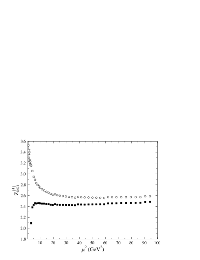
Figure 2: $Z^{\{5\}}_{\rm RGI}$ calculated in the $\overline{\rm MS}$ scheme (circles) and in a MOM scheme (filled squares) at $\beta=5.40$. The scale is fixed using $r_{0}=0.467$fm.

As mentioned above, the renormalization of the twist-3 operator in Eqs. (17), (18) has further complications due to the mixing effects described in Section II. In this case it is unclear how to convert our MOM results to the $\overline{\mbox{MS}}$ scheme. So we shall stick to the MOM numbers. For the comparison of our results with experimental determinations this does not cause problems, because no QCD corrections have been taken into account in the analysis of the experiments and hence different schemes are not distinguished.

In Fig. 3 we plot the ratio $Z^{\sigma}(a\mu)/Z^{[5]}(a\mu)$ as a function of $\mu$ for $\beta=5.40$. As expected, a plateau develops for larger values of $\mu$, and therefore the operator ${\cal O}^{[5]}(\mu)$ only depends on $\mu$ multiplicatively.

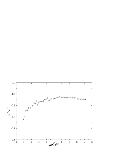
Figure 3: The ratio $Z^{\sigma}(a\mu)/Z^{[5]}(a\mu)$ at $\beta=5.40$

V Results for Reduced Matrix Elements

In order to compute the reduced matrix elements in Eqs. (LABEL:eq:twist2) and (LABEL:eq:twist3), we calculate the ratio of three- to two-point correlation functions ${\cal R}$, as given in Eq. (25), for the operators defined in Eqs. (16)-(20). The bare operator matrix elements are obtained from the ratio ${\cal R}$ by

$${\cal R}_{a_{2}}=\frac{1}{2\kappa_{\rm sea}}\frac{1}{6}M\,p\,a_{2}\,,\ {\cal R}_{d_{2}}=\frac{1}{2\kappa_{\rm sea}}\frac{1}{3}M\,p\,d_{2}\,.$$ (26)

We define the continuum quark fields by $\sqrt{2\kappa_{\rm sea}}$ times the lattice quark fields. The factor for ${\cal R}_{d_{2}}$ is the same for all three operators ${\cal O}^{[5]}$, ${\cal O}^{\sigma}$ and ${\cal O}^{0}$.

In Tables 2 and 3 we present our results for the bare matrix elements of the operators ${\cal O}^{\{5\}}$, ${\cal O}^{[5]}$, ${\cal O}^{\sigma}$ and ${\cal O}^{0}$ defined in Eqs. (16)-(20) for $u$ and $d$ quarks in the proton.

Table 2: Bare (unrenormalized) matrix elements $a_{2}$, $d_{2}^{[5]}$, for $u$ and $d$ quarks in the proton for our entire set of $(\beta,\,\kappa_{\rm sea})$ combinations.

$\beta$	$\kappa_{\rm sea}$	$a_{2}^{(u)}$	$a_{2}^{(d)}$	$d_{2}^{[5]\,(u)}$	$d_{2}^{[5]\,(d)}$
5.20	0.13420	$0.142(18)$	$-0.0318(78)$	$-0.0143(23)$	$0.0005(14)$
5.20	0.13500	$0.123(22)$	$-0.032(11)$	$-0.0329(59)$	$0.0094(35)$
5.20	0.13550	$0.131(32)$	$-0.061(22)$	$-0.057(14)$	$0.0064(59)$
5.25	0.13460	$0.113(12)$	$-0.0389(51)$	$-0.0165(25)$	$0.0023(13)$
5.25	0.13520	$0.110(19)$	$-0.0281(74)$	$-0.0310(39)$	$0.0069(17)$
5.25	0.13575	$0.1107(74)$	$-0.0345(47)$	$-0.0575(28)$	$0.0074(15)$
5.29	0.13400	$0.1141(77)$	$-0.0255(35)$	$-0.0033(11)$	$-0.00009(63)$
5.29	0.13500	$0.0989(90)$	$-0.0281(45)$	$-0.0252(19)$	$0.0046(11)$
5.29	0.13550	$0.1228(65)$	$-0.0302(26)$	$-0.0468(23)$	$0.00783(92)$
5.40	0.13500	$0.1195(44)$	$-0.0227(24)$	$-0.02135(99)$	$0.00232(61)$
5.40	0.13560	$0.1238(63)$	$-0.0331(34)$	$-0.0445(26)$	$0.0069(11)$
5.40	0.13610	$0.127(13)$	$-0.0277(60)$	$-0.0674(48)$	$0.0103(25)$

Table 3: Bare (unrenormalized) matrix elements $d_{2}^{\sigma}/a$ and $d_{2}^{0}$ for $u$ and $d$ quarks in the proton for our entire set of $(\beta,\,\kappa_{\rm sea})$ combinations.

$\beta$	$\kappa_{\rm sea}$	$d_{2}^{\sigma\,(u)}/a$	$d_{2}^{\sigma\,(d)}/a$	$d_{2}^{0\,(u)}$	$d_{2}^{0\,(d)}$
5.20	0.13420	$-0.220(19)$	$0.046(8)$	$-0.0312(46)$	$0.0096(22)$
5.20	0.13500	$-0.305(29)$	$0.077(13)$	$-0.039(10)$	$0.0145(49)$
5.20	0.13550	$-0.395(60)$	$0.080(21)$	$-0.063(14)$	$0.0194(75)$
5.25	0.13460	$-0.252(17)$	$0.045(6)$	$-0.0371(34)$	$0.0150(28)$
5.25	0.13520	$-0.239(23)$	$0.063(10)$	$-0.0329(61)$	$0.0131(42)$
5.25	0.13575	$-0.353(13)$	$0.0638(44)$	$-0.0463(39)$	$0.0141(20)$
5.29	0.13400	$-0.213(9)$	$0.0379(35)$	$-0.0322(23)$	$0.0086(12)$
5.29	0.13500	$-0.258(13)$	$0.0518(42)$	$-0.0312(34)$	$0.0118(21)$
5.29	0.13550	$-0.338(10)$	$0.0651(36)$	$-0.0390(25)$	$0.0120(13)$
5.40	0.13500	$-0.301(8)$	$0.0595(33)$	$-0.0396(18)$	$0.01231(84)$
5.40	0.13560	$-0.385(15)$	$0.0723(50)$	$-0.0502(26)$	$0.0137(15)$
5.40	0.13610	$-0.420(25)$	$0.087(9)$	$-0.0411(60)$	$0.0178(39)$

The corresponding renormalized (reduced) matrix elements for the renormalization scale $\mu^{2}=5\,\mbox{GeV}^{2}$ are given in Tables 4 and 5. While the superscripts $(u)$ and $(d)$ again refer to $u$ and $d$ quarks in the proton, the matrix elements for proton and neutron targets are denoted by $(p)$ and $(n)$, respectively. For $a_{2}$ the latter are given by

$$a_{2}^{(p)} = {\cal Q}^{(u)\,2}a_{2}^{(u)}+{\cal Q}^{(d)\,2}a_{2}^{(d)},$$ (27)

$$a_{2}^{(n)} = {\cal Q}^{(d)\,2}a_{2}^{(u)}+{\cal Q}^{(u)\,2}a_{2}^{(d)}$$ (28)

and similarly for $d_{2}$. The renormalized values of $d_{2}^{(f)}$ for $f=u,d$ in the proton are calculated from

$$d_{2}^{(f)}=Z^{[5]}d_{2}^{[5](f)}+\frac{1}{a}Z^{\sigma}d_{2}^{\sigma(f)}\,.$$ (29)

In the lines for $\kappa_{\rm sea}=\kappa_{c}$, Tables 4 and 5 contain results in the chiral limit, obtained by an extrapolation linear in $(r_{0}m_{\rm PS})^{2}$. The scale has been fixed from the value of $r_{0}/a$ at the respective quark masses using $r_{0}=0.467\,\mbox{fm}$. Alternatively, we could have worked with the chirally extrapolated values of $r_{0}/a$. This would increase $d_{2}^{(p)}$ and $d_{2}^{(u)}$ by up to twice the statistical error but would leave the other observables almost unaffected. On the other hand, setting $r_{0}=0.5\,\mbox{fm}$ or varying $r_{0}\Lambda_{\overline{\rm MS}}$ between 0.572 and 0.662 (corresponding to the combined statistical and systematic errors given in Ref. Gockeler:2005rv ) leads only to rather small changes in the final results.

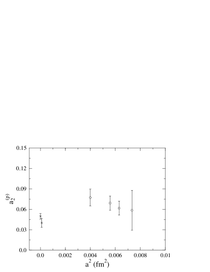
Figure 4: The chirally extrapolated reduced matrix element $a_{2}$ for the proton target renormalized at the scale $\mu^{2}\equiv Q^{2}=5$ GeV² as a function of the lattice spacing $a$. The crosses denote phenomenological determinations.

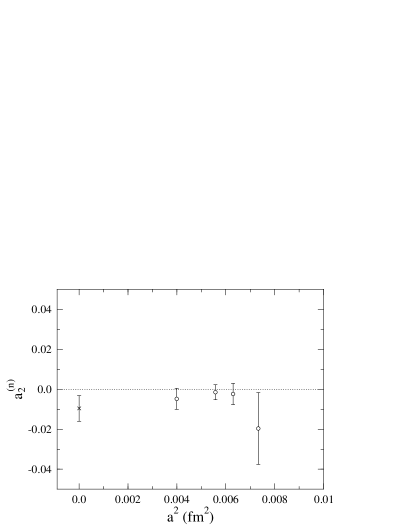
Figure 5: The chirally extrapolated reduced matrix element $a_{2}$ for the neutron target renormalized at the scale $\mu^{2}\equiv Q^{2}=5$ GeV² as a function of the lattice spacing $a$. The cross denotes the phenomenological value.

Let us first focus on the results for the twist-2 matrix element $a_{2}$. In Fig. 4 we show the chirally extrapolated renormalized results for $a_{2}$ in the proton in the $\overline{\mbox{MS}}$ scheme as a function of the lattice spacing $a$. It should however be noted that the data at $\beta=5.20$, i.e., those for the largest lattice spacing are to be considered with caution, because potentially they are affected by lattice artefacts. For $a_{2}$ the dependence on the quark mass turns out to be rather small. On the other hand, we do not attempt a continuum extrapolation of the chirally extrapolated results. Instead we take the value at our smallest lattice spacing ($\beta=5.4$) as our best estimate: $a_{2}^{(p)}=0.077(12)$. This is consistent with earlier quenched results QCDSF1 , indicating that quenching effects are small.

At the physical pion mass, we compare with two results taken from the literature which are obtained from an analysis of experimental data. The larger value is taken from an earlier analysis performed by Abe et al. exp2 , while the lower point is extracted from a recent analysis by Osipenko et al. Osipenko:2005nx with the help of the perturbative Wilson coefficient. In the $\overline{\mbox{MS}}$ scheme with anticommuting $\gamma_{5}$, we use the two-loop expression for the Wilson coefficient described in Ref. Zijlstra:1993sh . To avoid large logarithms, we set $Q^{2}=\mu^{2}=5$ GeV² to obtain

$$e^{(f)}_{1,2}={\cal Q}^{(f)2}\times 1.03075\,.$$ (30)

We do not see exact agreement between our chirally extrapolated value and those obtained from experimental data, but there are still several sources of systematic error in our final number. Firstly, our simulation only involves the calculation of connected quark diagrams. That is, we do not consider the (computationally expensive) case where an operator couples to a disconnected quark loop, although such disconnected diagrams are not expected to contribute in the large $x$ region. Secondly, our results are restricted to the heavy pion world, $m_{\rm PS}>550$ MeV. In this region we observe a linear dependence of our results on $m_{\rm PS}^{2}$. A more advanced functional form guided by chiral perturbation theory, such as those proposed for the moments of unpolarized nucleon structure functions Detmold or nucleon magnetic moments chiral , may be required. One such form has been suggested in Detmold:2002nf , but only for iso-vector matrix elements. So we attempt to gain an estimate of the systematic uncertainty due to our linear extrapolation by comparing results for $a_{2}^{(u-d)}$ in the chiral limit using both a linear extrapolation and the form proposed in Detmold:2002nf

$$a_{2}^{(u-d)}(m_{\pi}^{2}) = a_{2}^{(u-d)}\left(1+c_{\rm LNA}\,m_{\pi}^{2}\log\frac{m_{\pi}^{2}}{m_{\pi}^{2}+\mu^{2}}\right)$$ (31)

$$\qquad+b_{2}\frac{m_{\pi}^{2}}{m_{\pi}^{2}+m_{b}^{2}}\ ,$$

where the authors recommend a preferred value for the LNA coefficient as $c_{\rm LNA}=-(0.48g_{A}^{2}+1)/(4\pi f_{\pi})^{2}$ and $b_{2}$ is constrained by the heavy quark limit to be

$$b_{2}^{(u-d)}=\frac{5}{27}-a_{2}^{(u-d)}(1-\mu^{2}c_{\rm LNA})\ .$$ (32)

We set $\mu=0.25$ GeV as proposed in Detmold:2002nf and find at $\beta=5.29$, $a_{2}^{(u-d)}=0.214(29)$ employing a linear extrapolation and $a_{2}^{(u-d)}=0.183(9)$ using Eq. (31), suggesting there is a $15\%$ systematic error in our linear extrapolation.

Finally, we have not considered finite size effects Detmold:2005pt in this work, and our data do not yet allow us to perform a decent continuum extrapolation.

Table 4: Renormalized matrix elements for the renormalization scale $\mu^{2}=5\,\mbox{GeV}^{2}$ in the $\overline{\mbox{MS}}$ scheme. The superscripts $(u)$ and $(d)$ refer to $u$ and $d$ quarks in the proton.

$\beta$	$\kappa_{\rm sea}$	$a_{2}^{(u)}$	$a_{2}^{(d)}$	$d_{2}^{(u)}$	$d_{2}^{(d)}$
5.20	0.13420	$0.194(27)$	$-0.044(11)$	$0.0360(59)$	$-0.0113(29)$
5.20	0.13500	$0.168(32)$	$-0.044(15)$	$0.039(12)$	$-0.0082(65)$
5.20	0.13550	$0.179(45)$	$-0.083(30)$	$0.034(28)$	$-0.015(11)$
5.20	$\kappa_{c}$	$0.154(65)$	$-0.079(37)$	$0.040(31)$	$-0.011(14)$
5.25	0.13460	$0.154(19)$	$-0.0532(76)$	$0.0335(53)$	$-0.0070(24)$
5.25	0.13520	$0.150(27)$	$-0.038(10)$	$0.0109(79)$	$-0.0047(34)$
5.25	0.13575	$0.151(13)$	$-0.0472(70)$	$0.0024(54)$	$-0.0050(25)$
5.25	$\kappa_{c}$	$0.149(24)$	$-0.042(12)$	$-0.0169(89)$	$-0.0036(41)$
5.29	0.13400	$0.159(14)$	$-0.0356(53)$	$0.0468(27)$	$-0.0094(13)$
5.29	0.13500	$0.138(15)$	$-0.0392(67)$	$0.0284(43)$	$-0.0064(20)$
5.29	0.13550	$0.171(13)$	$-0.0421(43)$	$0.0201(44)$	$-0.0056(17)$
5.29	$\kappa_{c}$	$0.167(24)$	$-0.0469(84)$	$-0.0008(70)$	$-0.0026(28)$
5.40	0.13500	$0.170(12)$	$-0.0323(39)$	$0.0499(27)$	$-0.0127(13)$
5.40	0.13560	$0.176(13)$	$-0.0471(55)$	$0.0401(57)$	$-0.0097(22)$
5.40	0.13610	$0.181(21)$	$-0.0394(88)$	$0.019(10)$	$-0.0094(46)$
5.40	$\kappa_{c}$	$0.187(28)$	$-0.056(11)$	$0.010(12)$	$-0.0056(50)$

Table 5: Renormalized matrix elements for the renormalization scale $\mu^{2}=5\,\mbox{GeV}^{2}$ in the $\overline{\mbox{MS}}$ scheme. The superscripts $(p)$ and $(n)$ denote the matrix elements for proton and neutron targets, respectively.

$\beta$	$\kappa_{\rm sea}$	$a_{2}^{(p)}$	$a_{2}^{(n)}$	$d_{2}^{(p)}$	$d_{2}^{(n)}$
5.20	0.13420	$0.081(12)$	$0.0022(55)$	$0.0148(26)$	$-0.0010(14)$
5.20	0.13500	$0.070(14)$	$-0.0008(75)$	$0.0166(55)$	$0.0008(32)$
5.20	0.13550	$0.070(20)$	$-0.017(14)$	$0.013(13)$	$-0.0028(58)$
5.20	$\kappa_{c}$	$0.058(29)$	$-0.020(18)$	$0.017(14)$	$-0.0002(71)$
5.25	0.13460	$0.0627(82)$	$-0.0065(36)$	$0.0141(24)$	$0.0006(12)$
5.25	0.13520	$0.063(12)$	$-0.0004(53)$	$0.0043(36)$	$-0.0009(18)$
5.25	0.13575	$0.0620(58)$	$-0.0041(31)$	$0.0005(24)$	$-0.0019(13)$
5.25	$\kappa_{c}$	$0.062(10)$	$-0.0024(53)$	$-0.0079(40)$	$-0.0035(21)$
5.29	0.13400	$0.0668(61)$	$0.0019(25)$	$0.0198(12)$	$0.00105(64)$
5.29	0.13500	$0.0570(65)$	$-0.0021(31)$	$0.0119(19)$	$0.00031(99)$
5.29	0.13550	$0.0715(57)$	$0.0003(19)$	$0.0083(20)$	$-0.00028(89)$
5.29	$\kappa_{c}$	$0.069(10)$	$-0.0015(38)$	$-0.0006(31)$	$-0.0012(15)$
5.40	0.13500	$0.0720(50)$	$0.0045(17)$	$0.0208(12)$	$-0.00009(63)$
5.40	0.13560	$0.0731(58)$	$-0.0014(24)$	$0.0168(25)$	$0.0001(11)$
5.40	0.13610	$0.0760(93)$	$0.0026(43)$	$0.0072(46)$	$-0.0021(23)$
5.40	$\kappa_{c}$	$0.077(12)$	$-0.0048(53)$	$0.0039(54)$	$-0.0013(26)$

Our results for $a_{2}$ in the neutron are shown in Fig. 5. They are hardly different from zero. Taking again the value for $\beta=5.4$ as our best estimate, we end up with $a_{2}^{(n)}=-0.005(5)$, in agreement with the result from the analysis of Abe et al. exp2 .

From $a_{2}^{(p)}$ and $a_{2}^{(n)}$ in the chiral limit we calculate (see Eq. (LABEL:eq:ope-g1)) the second moment of the polarized structure function $g_{1}$ for the proton and neutron. Using the Wilson coefficient given in Eq. (30) we find

$$\int_{0}^{1}\mbox{d}x\,x^{2}g_{1}^{p}(x,Q^{2})\!\! = \!\!\frac{1.03075}{4}a_{2}^{p}=0.0170(18)\,,$$ (33)

$$\int_{0}^{1}\mbox{d}x\,x^{2}g_{1}^{n}(x,Q^{2})\!\! = \!\!\frac{1.03075}{4}a_{2}^{p}=-0.0013(8).$$ (34)

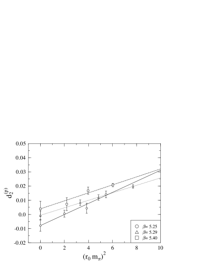
Figure 6: The chiral extrapolation of the reduced matrix element $d_{2}$ for the proton target renormalized at the scale $\mu^{2}\equiv Q^{2}=5$ GeV².

Figure 7: The chiral extrapolation of the reduced matrix element $d_{2}$ for the neutron target renormalized at the scale $\mu^{2}\equiv Q^{2}=5$ GeV².

We now turn our attention to the second moment of $g_{2}$. We find that our data for $d_{2}$ also exhibit a linear behavior in $m_{\rm PS}^{2}$. While this is not unexpected at the large pion masses where our simulations are performed, this linear behavior will not necessarily continue near the chiral limit. Unfortunately, the dependence of $d_{2}$ on the pion mass near the chiral limit is not yet known. Therefore in this work we perform only a linear extrapolation of $d_{2}$ to the chiral limit. In Figs. 6 and 7 we plot some of the data versus $(r_{0}m_{\rm PS})^{2}$ together with the linear extrapolations. The chirally extrapolated results for $d_{2}$ in the proton and neutron are shown in Figs. 8 and 9, respectively. At our smallest lattice spacing we obtain in the chiral limit

$$d_{2}^{(p)} = \phantom{-}0.004(5),$$ (35)

$$d_{2}^{(n)} = -0.001(3).$$ (36)

The errors are statistical only. Taking the behavior of $a_{2}^{(u-d)}$ as a guide, the chiral extrapolation might introduce a $15\%$ systematic uncertainty. For $d_{2}^{(p)}$ the other systematic uncertainties discussed above would amount to an additional error of about 0.005, while $d_{2}^{(n)}$ is almost unaffected. Our result for the proton agrees very well with the experimental number exp , while for the neutron the experimental result differs from ours by two standard deviations. A more precise experimental value would be most desirable in case of the neutron.

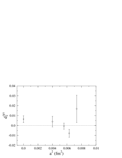
Figure 8: The chirally extrapolated reduced matrix element $d_{2}$ for the proton target renormalized at the scale $\mu^{2}\equiv Q^{2}=5$ GeV² as a function of the lattice spacing $a$. The cross denotes the phenomenological value.

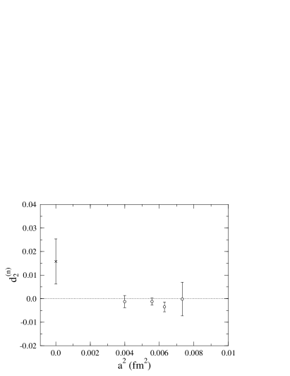
Figure 9: The chirally extrapolated reduced matrix element $d_{2}$ for the neutron target renormalized at the scale $\mu^{2}\equiv Q^{2}=5$ GeV² as a function of the lattice spacing $a$. The cross denotes the phenomenological value.

From Eq. (4), the moments of $g_{2}$ receive contributions from $g_{1}$ and $\overline{g_{2}}$, the second of which contains a mass dependent term and a gluon insertion dependent term. From Eq. (3), the second moment of $\overline{g_{2}}$ is (dropping the explicit $Q^{2}$ dependence)

$$\frac{1}{6}d_{2}=\int_{0}^{1}\mbox{d}x\,x^{2}\overline{g_{2}}(x)=\int_{0}^{1}\mbox{d}x\,x\frac{2}{3}\bigg{[}\frac{m}{M}h_{T}(x)+\xi(x)\bigg{]}\,,$$ (37)

so if $d_{2}$ vanishes in the chiral limit, then $\int_{0}^{1}\mathrm{d}xx\xi(x)$ must also vanish. Our results lead us to conclude that for the $n=2$ moment the Wandzura-Wilczek relation WW

$$\int_{0}^{1}\mbox{d}x\,x^{2}g_{2}(x,Q^{2})=-\frac{2}{3}\int_{0}^{1}\mbox{d}x\,x^{2}g_{1}(x,Q^{2})$$ (38)

is satisfied within errors for both proton and neutron targets.

From the expression in Eq. (3), we also expect the first moment of $\overline{g_{2}}$ to vanish in the chiral limit. Combining these two observations with the Burkhardt-Cottingham sum rule Burkhardt:1970ti , $\int_{0}^{1}g_{2}(x)\mbox{d}x=0$, and the knowledge that from elastic scattering processes $g_{2}$ receives non-trivial higher-twist contributions at $x=1$ (see, for example, Eqs. (4), (5) of Osipenko:2005nx ), we expect that there should be some sort of smooth transition at intermediate $x$, which presents an interesting challenge for the planned experiments at JLab JLab .

VI Conclusions

We have calculated the second moments of the proton and neutron’s spin-dependent $g_{1}$ and $g_{2}$ structure functions in lattice QCD with two flavors of ${\cal O}(a)$-improved Wilson fermions. A key feature of our investigation is the use of non-perturbative renormalization and the inclusion of operator mixing in our extraction of the twist-2 and twist-3 matrix elements.

Our result for $a_{2}^{(p)}=0.077(12)$ for the proton is somewhat larger than what follows from analyses of experimental data, while for the corresponding result for the neutron, we find a small but negative value, $a_{2}^{(n)}=-0.005(5)$, in agreement with experiment. Note that the errors are purely statistical and do not include any systematic uncertainties, although we estimate a systematic uncertainty of approximately $15\%$ arising from the chiral extrapolation.

For the twist-3 matrix element, $d_{2}$, our results agree very well with experiment and are consistent with zero, leading us to the conclusion that higher-twist effects occur only at large or intermediate $x$.

References

• (1) R. L. Jaffe, Comments Nucl. Part. Phys.  19, 239 (1990); R. L. Jaffe and X. D. Ji, Phys. Rev. D 43, 724 (1991); J. Blumlein and N. Kochelev, Nucl. Phys. B 498, 285 (1997) [arXiv:hep-ph/9612318].
• (2) S. Wandzura and F. Wilczek, Phys. Lett. B 72, 195 (1977).
• (3) J. L. Cortes, B. Pire and J. P. Ralston, Z. Phys. C 55, 409 (1992).
• (4) K. Abe et al. [E143 collaboration], Phys. Rev. D 58, 112003 (1998) [arXiv:hep-ph/9802357].
• (5) P. L. Anthony et al. [E155 Collaboration], Phys. Lett. B 553, 18 (2003) [arXiv:hep-ex/0204028].
• (6) B. Ehrnsperger, L. Mankiewicz and A. Schäfer, Phys. Lett. B 323, 439 (1994) [arXiv:hep-ph/9311285].
• (7) M. Göckeler et al., Phys. Rev. D 63, 074506 (2001) [arXiv:hep-lat/0011091].
• (8) M. Göckeler et al., Phys. Rev. D 53, 2317 (1996) [arXiv:hep-lat/9508004].
• (9) M. Göckeler et al., Nucl. Phys. B 472, 309 (1996) [arXiv:hep-lat/9603006].
• (10) G. Martinelli, C. Pittori, C. T. Sachrajda, M. Testa and A. Vladikas, Nucl. Phys. B 445, 81 (1995) [arXiv:hep-lat/9411010].
• (11) M. Göckeler et al., Nucl. Phys. B 544, 699 (1999) [arXiv:hep-lat/9807044].
• (12) M. Baake, B. Gemünden and R. Oedingen, J. Math. Phys.  23, 944 (1982) [Erratum-ibid.  23, 2595 (1982)]; J. E. Mandula, G. Zweig and J. Govaerts, Nucl. Phys. B 228, 109 (1983).
• (13) M. Göckeler, R. Horsley, D. Pleiter, P. E. L. Rakow and G. Schierholz [QCDSF Collaboration], arXiv:hep-ph/0410187.
• (14) M. Göckeler et al., arXiv:hep-ph/0502212.
• (15) M. Osipenko et al., Phys. Rev. D 71, 054007 (2005) [arXiv:hep-ph/0503018].
• (16) W. Detmold et al., Phys. Rev. Lett.  87, 172001 (2001) [arXiv:hep-lat/0103006]; J. W. Chen and X. Ji, Phys. Rev. Lett.  87, 152002 (2001) [Erratum-ibid.  88, 249901 (2002)] [arXiv:hep-ph/0107158]; D. Arndt and M. J. Savage, Nucl. Phys. A 697, 429 (2002) [arXiv:nucl-th/0105045].
• (17) M. Göckeler et al., [QCDSF Collaboration], Phys. Rev. D 71, 034508 (2005) [arXiv:hep-lat/0303019]; D. B. Leinweber, D. H. Lu and A. W. Thomas, Phys. Rev. D 60, 034014 (1999) [arXiv:hep-lat/9810005]; E. J. Hackett-Jones, D. B. Leinweber and A. W. Thomas, Phys. Lett. B 489, 143 (2000) [arXiv:hep-lat/0004006]; T. R. Hemmert and W. Weise, Eur. Phys. J. A 15, 487 (2002) [arXiv:hep-lat/0204005]; R. D. Young, D. B. Leinweber and A. W. Thomas, Phys. Rev. D 71, 014001 (2005) [arXiv:hep-lat/0406001].
• (18) W. Detmold, W. Melnitchouk and A. W. Thomas, Phys. Rev. D 66, 054501 (2002) [arXiv:hep-lat/0206001].
• (19) W. Detmold and C. J. Lin, Phys. Rev. D 71, 054510 (2005) [arXiv:hep-lat/0501007].
• (20) E. B. Zijlstra and W. L. van Neerven, Nucl. Phys. B 417, 61 (1994) [Erratum-ibid. B 426, 245 (1994)].
• (21) H. Burkhardt and W. N. Cottingham, Annals Phys.  56 (1970) 453.
• (22) Z.E. Meziani, private communication.
• (23) C. R. Allton et al. [UKQCD Collaboration], Phys. Rev. D 65, 054502 (2002) [arXiv:hep-lat/0107021].