NSF-KITP-05-08, UPRF-2005-01

Exact lattice Ward-Takahashi identity for the $N=1$ Wess-Zumino model

Marisa Bonini^a and Alessandra Feo^a,b

a. Dipartimento di Fisica, Università di Parma and INFN Gruppo Collegato di Parma,
Parco Area delle Scienze, 7/A, 43100 Parma, Italy
b. Kavli Institute for Theoretical Physics, UCSB, Santa Barbara, CA 93106, USA

Abstract

We consider a lattice formulation of the four dimensional $N=1$ Wess-Zumino model that uses the Ginsparg-Wilson relation. This formulation has an exact supersymmetry on the lattice. We show that the corresponding Ward-Takahashi identity is satisfied, both at fixed lattice spacing and in the continuum limit. The calculation is performed in lattice perturbation theory up to order $g^{2}$ in the coupling constant. We also show that this Ward-Takahashi identity determines the finite part of the scalar and fermion renormalization wave functions which automatically leads to restoration of supersymmetry in the continuum limit. In particular, these wave functions coincide in this limit.

Keywords: lattice gauge theory, supersymmetry, Wess-Zumino model.

PACS numbers:

1 Introduction

Recently, there have been several attempts to study supersymmetric theories on the lattice [1]-[3] (for recent reviews and a complete list of references, see [4]). The major obstacle in formulating a supersymmetric theory on the lattice arises from the fact that the supersymmetry algebra, which is actually an extension of the Poincaré algebra, is explicitly broken by the space-time discretization. Without exact lattice supersymmetry one might hope to construct non-supersymmetric lattice theories with a supersymmetric continuum limit. This is the case of the Wilson fermion approach for the $N=1$ supersymmetric Yang-Mills theory [3] where the only operator that violates the $N=1$ supersymmetry is a fermion mass term. By tuning the fermion mass to the supersymmetric limit one recovers supersymmetry in the continuum limit (see Ref. [5] for numerical studies along this approach).

The strategy of most recent studies is to realize part of the supercharges as an exact symmetry on the lattice. This exact supersymmetry is expected to play a key role to restore the continuum supersymmetry without (or with less) fine-tuning of the action parameters. These ideas apply to theories with extended supersymmetry where the lattice theory is realized by an orbifolding construction [6, 7]. Another approach is based on writing the theory in terms of twisted fields [8, 9]. The connection between twisted fields and Kähler-Dirac fermions is emphasized in [10] and recently in [11].

In this paper we consider the $N=1$ four dimensional lattice Wess-Zumino model introduced in Refs. [12, 13] and studied in [14] where it was shown that it is actually possible to define a lattice supersymmetry transformation which leaves invariant the full action at fixed lattice spacing. This transformation is non-linear in the scalar field. The action and the transformation are written in terms of the Ginsparg-Wilson operator and reduce to their continuum expression in the naive continuum limit $a\to 0$. In [14] the algebra of this lattice supersymmetry transformation was studied and the closure of the algebra was explicitly shown to $g^{2}$ order. This is a necessary ingredient to guarantee the request of supersymmetry. It was also argued that the existence of this exact symmetry is responsible for the restoration of supersymmetry in the continuum limit. In this paper, we derive the Ward-Takahashi identity (WTi) associated with this lattice supersymmetry transformation and show how in the continuum limit one recovers the WTi associated with the continuum supersymmetry transformation. This will be done in lattice perturbation theory up to order $g^{2}$. An outcome of this approach is the calculation of the lattice renormalization wave function for the scalar and fermion fields.

The paper is organized as follows. In Sec. 2 we briefly review the $N=1$ four dimensional lattice Wess-Zumino model based on the Ginsparg-Wilson fermion operator, and show how to build up a lattice supersymmetry transformation which is an exact symmetry of the lattice action. In Sec. 3 we derive the WTi and we explicitly check the simplest one, the one-point WTi at one-loop. A second and more interesting WTi, relating the boson and fermion two-point function, is analyzed at $g^{2}$ order in Sec. 4. Here it is shown that this identity is exactly satisfied on the lattice. In Sec. 5 we verify this WTi in the continuum limit and determine the finite part of the lattice renormalization constants which allow to identify the continuum invariant theory. Technical details of the fermion Dirac operator and the tadpole cancellations are presented in Appendix A and B, respectively.

2 The Wess-Zumino model

We formulate the lattice Wess-Zumino model by introducing a Dirac operator which satisfies the Ginsparg-Wilson relation [15]

$$\gamma_{5}D+D\gamma_{5}=aD\gamma_{5}D\,.$$ (1)

This relation implies the existence of a continuum symmetry of the fermion action which may be regarded as a lattice form of the chiral symmetry [16] and protects the fermion masses from additive renormalization. As shown in Ref. [13], using this Dirac operator it is possible to introduce a local action which is chiral invariant and where the fermions satisfy the Majorana condition. Moreover, in order to keep as much as symmetry as possible, the bosonic kinetic operator must be written in terms of $D$. The lattice action for the Wess-Zumino action reads

$$S_{WZ}=S_{0}+S_{int}\,,$$ (2)

with

$$S_{0}=\sum_{x}\bigg{\{}\frac{1}{2}\bar{\chi}(1-\frac{a}{2}D_{1})^{-1}D_{2}\chi-\frac{1}{a}(AD_{1}A+BD_{1}B)$$

$$\phantom{S_{0}=\sum_{x}\bigg{\{}}+\frac{1}{2}F(1-\frac{a}{2}D_{1})^{-1}F+\frac{1}{2}G(1-\frac{a}{2}D_{1})^{-1}G\bigg{\}}\,,$$ (3)

$$S_{int}=\sum_{x}\bigg{\{}\frac{1}{2}m\bar{\chi}\chi+m(FA+GB)+\frac{1}{\sqrt{2}}g\bar{\chi}(A+i\gamma_{5}B)\chi$$

$$\phantom{S_{int}=\sum_{x}\bigg{\{}}+\frac{1}{\sqrt{2}}g\big{[}F(A^{2}-B^{2})+2G(AB)\big{]}\bigg{\}}\,,$$ (4)

where $A$, $B$, $F$ and $G$ are real scalar fields and $\chi$ is a Majorana fermion which satisfies the Majorana condition

$$\bar{\chi}=\chi^{T}C$$ (5)

and $C$ is the charge conjugation matrix which satisfies

$$C^{T}=-C\,,\qquad\qquad CC^{\dagger}=1\,.$$ (6)

Moreover, our conventions are

$$C\gamma_{\mu}C^{-1}=-(\gamma_{\mu})^{T}\,,$$

$$C\gamma_{5}C^{-1}=(\gamma_{5})^{T}\,.$$ (7)

The operators $D_{1}$ and $D_{2}$ which enter in $S_{0}$ are related to the operator $D$ in (1) by

$$D_{1}=\frac{1}{4}\mbox{Tr}(D)\,,\;\;\;\;\;\;\;\;\;\;D_{2}=\frac{1}{4}\gamma_{\mu}\mbox{Tr}(\gamma_{\mu}D)\,.$$ (8)

Our analysis is valid for all operators that satisfy Eq. (1), however, in the following we will use the particularly simple solution given by Neuberger [17]

$$D=\frac{1}{a}\bigg{(}1-X\frac{1}{\sqrt{X^{\dagger}X}}\bigg{)}\,,\qquad\qquad X=1-aD_{w}\,,$$ (9)

where

$$D_{w}=\frac{1}{2}\gamma_{\mu}(\nabla^{\star}_{\mu}+\nabla_{\mu})-\frac{a}{2}\nabla^{\star}_{\mu}\nabla_{\mu}$$ (10)

and

$$\nabla_{\mu}\phi(x) = \frac{1}{a}(\phi(x+a\hat{\mu})-\phi(x))\,,$$

$$\nabla_{\mu}^{\star}\phi(x) = \frac{1}{a}(\phi(x)-\phi(x-a\hat{\mu}))$$ (11)

are the forward and backward lattice derivatives, respectively. Substituting Eq. (9) in Eq. (8) one finds

$$D_{1}=\frac{1}{a}\bigg{[}1-(1+\frac{a^{2}}{2}\nabla^{\star}_{\mu}\nabla_{\mu})\frac{1}{\sqrt{X^{\dagger}X}}\bigg{]}\,,\qquad\qquad D_{2}=\frac{1}{2}\gamma_{\mu}(\nabla^{\star}_{\mu}+\nabla_{\mu})\frac{1}{\sqrt{X^{\dagger}X}}\equiv\gamma_{\mu}D_{2\mu}\,.$$ (12)

The Ginsparg-Wilson relation (1) implies the following relations for $D_{1}$ and $D_{2}$

$$D_{1}^{2}-D_{2}^{2}=\frac{2}{a}D_{1}$$ (13)

and

$$(1-\frac{a}{2}D_{1})^{-1}D_{2}^{2}=-\frac{2}{a}D_{1}\,.$$ (14)

Before concluding this section we list the propagators of the lattice perturbation theory for the scalar and fermion fields:

$$\langle AA\rangle = \langle BB\rangle=-{\cal M}^{-1}(1-\frac{a}{2}D_{1})^{-1}$$

$$\langle FF\rangle = \langle GG\rangle=\frac{2}{a}{\cal M}^{-1}D_{1}=-{\cal M}^{-1}(1-\frac{a}{2}D_{1})^{-1}D_{2}^{2}$$

$$\langle AF\rangle = \langle BG\rangle=m\,{\cal M}^{-1}$$

$$\langle\chi\bar{\chi}\rangle = ((1-\frac{a}{2}D_{1})^{-1}D_{2}+m)^{-1}=-{\cal M}^{-1}((1-\frac{a}{2}D_{1})^{-1}D_{2}-m)\,,$$ (15)

where

$${\cal M}=\Big{[}\frac{2}{a}D_{1}(1-\frac{a}{2}D_{1})^{-1}+m^{2}\Big{]}$$ (16)

and the Ginsparg-Wilson relation (14) has been used to rewrite the auxiliary fields propagators. Despite the appearance of the operator $(1-\frac{a}{2}D_{1})^{-1}$, there are no would be doublers and the propagators are regular (see appendix A).

2.1 The supersymmetric transformation

As discussed in [12], $S_{0}$ is invariant under a lattice supersymmetry transformation which is obtained from the continuum one by replacing the continuum derivative with the lattice derivative $D_{2\mu}$. On the contrary the interaction term $S_{int}$ breaks this symmetry because of the failure of the Leibniz rule at finite lattice spacing [1]. In order to discuss the symmetry properties of the lattice Wess-Zumino model one possibility is to modify the action by adding irrelevant terms which make invariant the full action. Alternatively, one can modify the supersymmetry transformation in such a way that the action (2) has an exact symmetry for fixed $a$. In [14] it has been shown that the full action (2) is invariant under the following supersymmetry transformation

$$\delta A=\bar{\varepsilon}\chi=\bar{\chi}\varepsilon$$

$$\delta B=-i\bar{\varepsilon}\gamma_{5}\chi=-i\bar{\chi}\gamma_{5}\varepsilon$$

$$\delta\chi=-D_{2}(A-i\gamma_{5}B)\varepsilon-(F-i\gamma_{5}G)\varepsilon+gR\varepsilon$$

$$\delta F=\bar{\varepsilon}D_{2}\chi$$

$$\delta G=i\bar{\varepsilon}D_{2}\gamma_{5}\chi\,,$$ (17)

where $R$ is a function depending on the scalar fields and their derivatives that can be determined in perturbation theory imposing the invariance of the Wess-Zumino action under (17).

By expanding $R$ in powers of $g$,

$$R=R^{(1)}+gR^{(2)}+\cdots$$ (18)

and imposing the symmetry condition order by order in perturbation theory, one finds

$$R^{(1)}=((1-\frac{a}{2}D_{1})^{-1}D_{2}+m)^{-1}\Delta L$$ (19)

with

$$\Delta L\equiv\frac{1}{\sqrt{2}}\Big{\{}2(AD_{2}A-BD_{2}B)-D_{2}(A^{2}-B^{2})+2i\gamma_{5}\Big{[}(AD_{2}B+BD_{2}A)-D_{2}(AB)\Big{]}\Big{\}}$$ (20)

and

$$R^{(n)}=-\sqrt{2}((1-\frac{a}{2}D_{1})^{-1}D_{2}+m)^{-1}(A+i\gamma_{5}B)R^{(n-1)}\,,$$ (21)

for $n\geq 2$. Notice that the operator $((1-\frac{a}{2}D_{1})^{-1}D_{2}+m)^{-1}$ is precisely the free fermion propagator and that the transformation (17), like the function $R$, is non-linear in the scalar fields. Indeed, using (19) and (21) one sees that the expansion (18) can be resummed and $R$ is the formal solution of the equation

$$\big{[}(1-\frac{a}{2}D_{1})^{-1}D_{2}+m+\sqrt{2}g(A+i\gamma_{5}B)\big{]}R=\Delta L\,.$$ (22)

Notice that, in the limit $a\to 0$ the transformation (17) reduces to the continuum supersymmetry transformation, since $\Delta L$ vanishes in this limit. Indeed, $\Delta L$ is different from zero because of the breaking of the Leibniz rule at finite lattice spacing.

In [14] it has been shown that the algebra associated with the lattice supersymmetry transformation (17) closes. The existence of this exact symmetry should be responsible for the restoration of supersymmetry in the continuum limit.

In the following sections we will prove that the Ward-Takahashi identity (WTi) derived from this lattice supersymmetry is exactly satisfied at finite lattice spacing. We will perform a one-loop analysis though the procedure can be generalized to higher loops. We will also discuss the $a\to 0$ limit.

3 One-point Ward-Takahashi

The WTi is derived from the generating functional

$$Z[\Phi,J]=\int{\cal D}\Phi\exp{-(S_{WZ}+S_{J})}$$ (23)

where $S_{J}$ is the source term

$$S_{J}=\sum_{x}J_{\Phi}\cdot\Phi\equiv\sum_{x}\Bigg{\{}J_{A}\,A+J_{B}\,B+J_{F}\,F+J_{G}\,G+\bar{\eta}\chi\Bigg{\}}\,.$$ (24)

Using the invariance of both the Wess-Zumino action and the measure with respect to the lattice supersymmetry transformation (17), the WTi reads

$$\langle J_{\Phi}\cdot\delta\Phi\rangle_{J}=0\,,$$ (25)

with $\delta\Phi$ given in (17).

We begin with the simplest WTi which is obtained by taking the derivative with respect to $\bar{\eta}$ and setting to zero all the sources

$$\langle D_{2}(A-i\gamma_{5}B)\rangle+\langle F\rangle-i\gamma_{5}\langle G\rangle-g\langle R\rangle=0\,.$$ (26)

The order $O(g)$ of this Ward-Takahashi identity is

$$\langle D_{2}(A-i\gamma_{5}B)\rangle^{(1)}+\langle F\rangle^{(1)}-i\gamma_{5}\langle G\rangle^{(1)}-g\langle R^{(1)}\rangle^{(0)}=0\,,$$ (27)

where the notation $\langle{\cal O}\rangle^{(n)}$ indicates the $n-$order (in $g$) contribution to the expectation value of ${\cal O}$. From Eq. (2) it is easy to see that all the terms of the WTi (27) are zero. For instance

$$\langle D_{2}A\rangle^{(1)}\sim D_{2xy}\Bigg{[}\langle A_{y}F_{u}\rangle\big{[}\langle A_{u}A_{u}\rangle-\langle B_{u}B_{u}\rangle\big{]}+\langle A_{y}A_{u}\rangle\big{[}2\langle A_{u}F_{u}\rangle+2\langle B_{u}G_{u}\rangle+\mbox{Tr}\langle\bar{\chi}_{u}\chi_{u}\rangle\big{]}\Bigg{]}=0$$ (28)

and similarly

$$\langle F_{x}\rangle^{(1)}\sim\langle F_{x}F_{u}\rangle\big{[}\langle A_{u}A_{u}\rangle-\langle B_{u}B_{u}\rangle\big{]}+\langle F_{x}A_{u}\rangle\big{[}2\langle A_{u}F_{u}\rangle+2\langle B_{u}G_{u}\rangle+\mbox{Tr}\langle\bar{\chi}_{u}\chi_{u}\rangle\big{]}=0\,.$$ (29)

The Feynman diagrams corresponding to the different contributions in (29) are depicted in fig. 1.

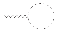
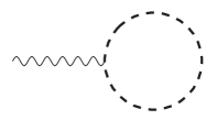
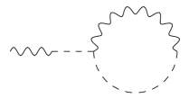
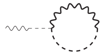
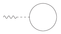
Figure 1: Tadpole cancellation. The (bold) curly and (bold) dashed lines denote the auxiliary field ($G$) $F$ and the scalar field ($B$) $A$, respectively; the solid line denotes the fermion field.

The vanishing of the $A$ and $F$ one-point functions is due to the exact cancellation of the tadpole diagrams on the lattice. Similarly, the $G$ and $B$ one-point functions are zero at this order due to the presence of a matrix $\gamma_{5}$ inserted in the fermion loop. In order to prove the WTi (27) one has to show that also the contribution depending on $R$ vanishes. Indeed one finds

$$\langle R^{(1)}\rangle^{(0)}=((1-\frac{a}{2}D_{1})^{-1}D_{2}+m)^{-1}\langle\Delta L_{y}\rangle^{(0)}$$

$$=\langle\chi_{x}\bar{\chi}_{y}\rangle\bigg{[}2\langle A_{y}D_{2yz}A_{z}\rangle-2\langle B_{y}D_{2yz}B_{z}\rangle-D_{2yz}\langle A_{z}A_{z}\rangle+D_{2yz}\langle B_{z}B_{z}\rangle\bigg{]}=0\,,$$ (30)

where (2) has been used.

4 Two-point Ward-Takahashi identity

In this section we discuss a more interesting WTi that relates the fermion and scalar two-point functions. Taking the derivative of (25) with respect to $\bar{\eta}$ and $J_{A}$ and setting to zero all the sources one obtains

$$\langle\chi_{y}\bar{\chi}_{x}\rangle-\langle D_{2yz}(A_{z}-i\gamma_{5}B_{z})A_{x}\rangle-\langle(F_{y}-i\gamma_{5}G_{y})A_{x}\rangle+g\langle R_{y}A_{x}\rangle=0\,.$$ (31)

Making use of the propagators given in (2), this identity is trivially satisfied at tree level.

The next non-trivial order is $g^{2}$ which corresponds to the one-loop diagrams and can be written as

$$\langle\chi_{y}\bar{\chi}_{x}\rangle^{(2)}-\langle D_{2yz}(A_{z}-i\gamma_{5}B_{z})A_{x}\rangle^{(2)}-\langle(F_{y}-i\gamma_{5}G_{y})A_{x}\rangle^{(2)}+g\bigg{(}\langle R^{(1)}_{y}A_{x}\rangle^{(1)}+g\langle R^{(2)}_{y}A_{x}\rangle^{(0)}\bigg{)}=0\,,$$ (32)

where we used the expansion (18) for the function $R$.

Applying the Wick expansion, the first term of this WTi is

$$\langle\chi_{y}\bar{\chi}_{x}\rangle^{(2)}=\frac{g^{2}}{4}\langle\chi_{y}\bar{\chi}_{x}\sum_{zu}\Big{[}\bar{\chi}(A+i\gamma_{5}B)\chi+F(A^{2}-B^{2})+2GAB\Big{]}_{z}$$

$$\phantom{<\chi_{y}\bar{\chi}_{x}>^{(2)}=\frac{g^{2}}{4}<\chi_{y}\bar{\chi}_{x}}\times\Big{[}\bar{\chi}(A+i\gamma_{5}B)\chi+F(A^{2}-B^{2})+2GAB\Big{]}_{u}\rangle^{(0)}\,.$$ (33)

We first isolate among the various contributions the tadpole ones

$$\langle\chi_{y}\bar{\chi}_{x}\rangle^{(2)}_{T}=g^{2}\sum_{zu}\Big{\{}\langle\chi_{y}\bar{\chi}_{z}\rangle\langle\chi_{z}\bar{\chi}_{x}\rangle\Big{[}\langle A_{z}F_{u}\rangle\Big{(}\langle A_{u}A_{u}\rangle-\langle B_{u}B_{u}\rangle\Big{)}$$

$$\phantom{\langle\chi_{y}\bar{\chi}_{x}\rangle^{(2)}_{T}=g^{2}\Big{\{}}+2\langle A_{z}A_{u}\rangle\Big{(}\langle A_{u}F_{u}\rangle+\langle B_{u}G_{u}\rangle\Big{)}-\langle A_{z}A_{u}\rangle\mbox{Tr}\langle\chi_{u}\bar{\chi}_{u}\rangle\Big{]}$$

$$\phantom{\langle\chi_{y}\bar{\chi}_{x}\rangle^{(2)}_{T}=g^{2}\Big{\{}}+\langle\chi_{y}\bar{\chi}_{z}\rangle\gamma_{5}\langle\chi_{z}\bar{\chi}_{x}\rangle\langle B_{z}B_{u}\rangle\mbox{Tr}\langle\chi_{u}\gamma_{5}\bar{\chi}_{u}\rangle\Big{\}}\,.$$ (34)

Using the propagators (2) and the relations $\mbox{Tr}\langle\chi\gamma_{5}\bar{\chi}\rangle=0$ and $\mbox{Tr}\langle\chi\bar{\chi}\rangle=4\langle AF\rangle=4\langle GB\rangle$, it is easy to demonstrate that the tadpole contributions cancel out (see Appendix B). This property is general and also holds for the other terms of the WTi (32). Therefore, one is left with the connected non tadpoles diagrams

$$\langle\chi_{y}\bar{\chi}_{x}\rangle^{(2)}_{NT}=2g^{2}\sum_{uz}\Big{\{}\langle\chi_{y}\bar{\chi}_{z}\rangle\langle\chi_{z}\bar{\chi}_{u}\rangle\langle\chi_{u}\bar{\chi}_{x}\rangle\langle A_{z}A_{u}\rangle-\langle\chi_{y}\bar{\chi}_{z}\rangle\gamma_{5}\langle\chi_{z}\bar{\chi}_{u}\rangle\gamma_{5}\langle\chi_{u}\bar{\chi}_{x}\rangle\langle B_{z}B_{u}\rangle\Big{\}}\,.$$ (35)

The corresponding Feynman diagrams are given in fig. 2.

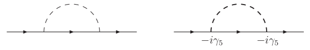
Figure 2: Non-tadpole contributions to $\langle\chi\bar{\chi}\rangle^{(2)}$.

The non-tadpole contributions to the second term of (32) are (here and in the following the sum over repeated indices $z,u,w$ is understood)

$$\langle D_{2yz}(A_{z}-i\gamma_{5}B_{z})A_{x}\rangle^{(2)}_{NT}=g^{2}\Big{\{}D_{2yz}\langle A_{z}A_{u}\rangle\Big{[}\mbox{Tr}\Big{(}\langle\chi_{u}\bar{\chi}_{w}\rangle\langle\chi_{w}\bar{\chi}_{u}\rangle\Big{)}+2\langle A_{u}A_{w}\rangle\langle F_{u}F_{w}\rangle$$

$$\phantom{\langle D_{2yz}(A_{z}-i\gamma_{5}}+2\langle B_{u}B_{w}\rangle\langle G_{u}G_{w}\rangle+2\langle F_{u}A_{w}\rangle\langle A_{u}F_{w}\rangle+2\langle B_{u}G_{w}\rangle\langle G_{u}B_{w}\rangle\Big{]}\langle A_{w}A_{x}\rangle$$

$$\phantom{\langle D_{2yz}(A_{z}-i\gamma_{5}}+D_{2yz}\langle A_{z}F_{u}\rangle\Big{[}\langle A_{u}A_{w}\rangle\langle A_{u}A_{w}\rangle+\langle B_{u}B_{w}\rangle\langle B_{u}B_{w}\rangle\Big{]}\langle F_{w}A_{x}\rangle$$

$$\phantom{\langle D_{2yz}(A_{z}-i\gamma_{5}}+2D_{2yz}\langle A_{z}F_{u}\rangle\Big{[}\langle A_{u}A_{w}\rangle\langle A_{u}F_{w}\rangle-\langle B_{u}B_{w}\rangle\langle B_{u}G_{w}\rangle\Big{]}\langle A_{w}A_{x}\rangle$$

$$\phantom{\langle D_{2yz}(A_{z}-i\gamma_{5}}+2D_{2yz}\langle A_{z}A_{u}\rangle\Big{[}\langle A_{u}A_{w}\rangle\langle F_{u}A_{w}\rangle-\langle B_{u}B_{w}\rangle\langle G_{u}B_{w}\rangle\Big{]}\langle F_{w}A_{x}\rangle\Big{\}}\,.$$ (36)

The corresponding Feynman diagrams are given in fig. 3.

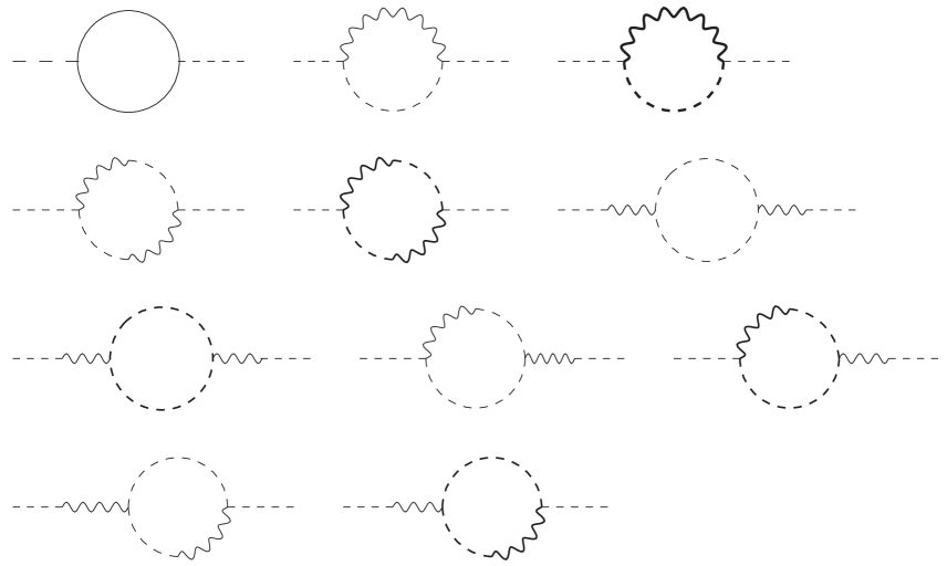
Figure 3: Non-tadpole contributions to $\langle D_{2}(A-i\gamma_{5}B)A\rangle^{(2)}$.

The non-tadpole contributions to the third term of (32) are

$$\langle(F_{y}-i\gamma_{5}G_{y})A_{x}\rangle^{(2)}_{NT}=g^{2}\Big{\{}2\langle F_{y}A_{u}\rangle\Big{[}\frac{1}{2}\mbox{Tr}\Big{(}\langle\chi_{u}\bar{\chi}_{w}\rangle\langle\chi_{w}\bar{\chi}_{u}\rangle\Big{)}+\langle F_{u}F_{w}\rangle\langle A_{u}A_{w}\rangle$$

$$\phantom{\langle(F_{y}-i\gamma_{5}G_{y})A_{x}\rangle^{(2)}_{NT}}+\langle F_{u}A_{w}\rangle\langle A_{u}F_{w}\rangle+\langle G_{u}G_{w}\rangle\langle B_{u}B_{w}\rangle+\langle B_{u}G_{w}\rangle\langle G_{u}B_{w}\rangle\Big{]}\langle A_{w}A_{x}\rangle$$

$$\phantom{\langle(F_{y}-i\gamma_{5}G_{y})A_{x}\rangle^{(2)}_{NT}}+\langle F_{y}F_{u}\rangle\Big{[}\langle A_{u}A_{w}\rangle\langle A_{u}A_{w}\rangle+\langle B_{u}B_{w}\rangle\langle B_{u}B_{w}\rangle\Big{]}\langle F_{w}A_{x}\rangle$$

$$\phantom{\langle(F_{y}-i\gamma_{5}G_{y})A_{x}\rangle^{(2)}_{NT}}+2\langle F_{y}A_{u}\rangle\Big{[}\langle F_{u}A_{w}\rangle\langle A_{u}A_{w}\rangle-\langle G_{u}B_{w}\rangle\langle B_{u}B_{w}\rangle\Big{]}\langle F_{w}A_{x}\rangle$$

$$\phantom{\langle(F_{y}-i\gamma_{5}G_{y})A_{x}\rangle^{(2)}_{NT}}+2\langle F_{y}F_{u}\rangle\Big{[}\langle A_{u}A_{w}\rangle\langle A_{u}F_{w}\rangle-\langle B_{u}B_{w}\rangle\langle B_{u}G_{w}\rangle\Big{]}\langle A_{w}A_{x}\rangle$$

$$\phantom{\langle(F_{y}-i\gamma_{5}G_{y})A_{x}\rangle^{(2)}_{NT}}-\gamma_{5}\langle G_{y}B_{w}\rangle\mbox{Tr}\Big{(}\gamma_{5}\langle\bar{\chi}_{w}\chi_{u}\rangle\langle\bar{\chi}_{u}\chi_{w}\rangle\Big{)}\langle A_{u}A_{x}\rangle\Big{\}}$$ (37)

and the corresponding Feynman diagrams are given in fig. 4.

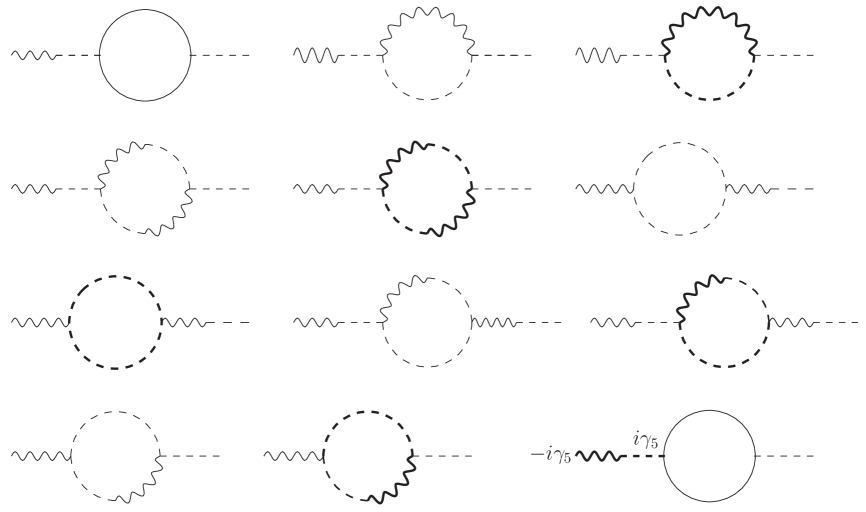
Figure 4: Non-tadpole contributions to $\langle(F-i\gamma_{5}G)A\rangle^{(2)}$.

Notice that the terms in last two rows of (4) cancel out since $\langle AA\rangle=\langle BB\rangle$ and $\langle AF\rangle=\langle BG\rangle$. These terms, originating from the last four diagrams in fig. 3, are the one-loop contribution to the 1PI $AF$-vertex function, which therefore vanishes at this order. Similarly, the last three rows of (4) do not contribute. In particular the last term, i.e. the last diagram of fig. 4 vanishes and that gives $\langle G_{y}A_{x}\rangle^{(2)}=0$.

For the terms of the WTi (32) involving the function $R$ one finds

$$\langle R_{y}^{(1)}A_{x}\rangle^{(1)}=-\frac{g}{\sqrt{2}}\langle\chi\bar{\chi}\rangle_{yz}\langle\Delta L_{z}\big{[}\bar{\chi}(A+i\gamma_{5}B)\chi+F(A^{2}-B^{2})+2GAB\big{]}_{u}A_{x}\rangle^{(0)}\,,$$ (38)

where the fermion propagator follows from (19).

Also in this case the tadpole diagrams cancel out and one is left with

$$\langle R_{y}^{(1)}A_{x}\rangle^{(1)}_{NT}=-g\langle\chi\bar{\chi}\rangle_{yz}$$ (39)

$$\phantom{\langle R_{y}^{(1)}A_{x}\rangle^{(1)}_{NT}}\times\Big{\{}2\Big{[}\langle A_{z}F_{w}\rangle D_{2zu}\langle A_{u}A_{w}\rangle+\langle A_{z}A_{w}\rangle D_{2zu}\langle A_{u}F_{w}\rangle-D_{2zu}\langle A_{u}F_{w}\rangle\langle A_{u}A_{w}\rangle$$

$$\phantom{\langle R_{y}^{(1)}A_{x}\rangle^{(1)}_{NT}}-\langle B_{z}G_{w}\rangle D_{2zu}\langle B_{u}B_{w}\rangle-\langle B_{z}B_{w}\rangle D_{2zu}\langle B_{u}G_{w}\rangle+D_{2zu}\langle B_{u}B_{w}\rangle\langle B_{u}G_{w}\rangle\Big{]}\langle A_{w}A_{x}\rangle$$

$$\phantom{\langle R_{y}^{(1)}A_{x}\rangle^{(1)}_{NT}}+\Big{[}2\langle A_{z}A_{w}\rangle D_{2zu}\langle A_{u}A_{w}\rangle-D_{2zu}\langle A_{u}A_{w}\rangle\langle A_{u}A_{w}\rangle$$

$$\phantom{\langle R_{y}^{(1)}A_{x}\rangle^{(1)}_{NT}+\Big{[}}+2\langle B_{z}B_{w}\rangle D_{2zu}\langle B_{u}B_{w}\rangle-D_{2zu}\langle B_{u}B_{w}\rangle\langle B_{u}B_{w}\rangle\Big{]}\langle F_{w}A_{x}\rangle\Big{\}}\,.$$

The corresponding Feynman diagrams are given in fig. 5.

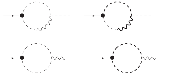
Figure 5: Non-tadpole contributions to $\langle R^{(1)}A\rangle^{(1)}$. The blob denotes the insertion of the operator $D_{2}$ acting on the three legs outgoing from the vertex as in equation (39).

Finally, for the last term of (32) one gets

$$\langle R_{y}^{(2)}A_{x}\rangle^{(0)}=-\sqrt{2}\langle\chi\bar{\chi}\rangle_{yz}\langle(A_{z}+i\gamma_{5}B_{z})\langle\chi\bar{\chi}\rangle_{zw}\Delta L_{w}A_{x}\rangle^{(0)}$$

$$\phantom{\langle R_{y}^{(2)}A_{x}\rangle^{(0)}}=-2\Big{\{}\langle\chi_{y}\bar{\chi}_{z}\rangle\langle\chi_{z}\bar{\chi}_{w}\rangle\Big{[}\langle A_{z}A_{w}\rangle D_{2wu}\langle A_{u}A_{x}\rangle+\langle A_{w}A_{x}\rangle D_{2wu}\langle A_{z}A_{u}\rangle$$

$$\phantom{\langle R_{y}^{(2)}A_{x}\rangle^{(0)}=-2\sqrt{2}\Big{\{}\langle\chi_{y}\bar{\chi}_{z}\rangle\langle\chi_{z}\bar{\chi}_{w}\rangle}-D_{2wu}\langle A_{z}A_{u}\rangle\langle A_{u}A_{x}\rangle\Big{]}$$

$$\phantom{\langle R_{y}^{(2)}A_{x}\rangle^{(0)}=}-\langle\chi_{y}\bar{\chi}_{z}\rangle\gamma_{5}\langle\chi_{z}\bar{\chi}_{w}\rangle\gamma_{5}\Big{[}\langle B_{z}B_{w}\rangle D_{2wu}\langle A_{u}A_{x}\rangle+\langle A_{w}A_{x}\rangle D_{2wu}\langle B_{z}B_{u}\rangle$$

$$\phantom{\langle R_{y}^{(2)}A_{x}\rangle^{(0)}=-2\sqrt{2}\Big{\{}\langle\chi_{y}\bar{\chi}_{z}\rangle\langle\chi_{z}\bar{\chi}_{w}\rangle}-D_{2wu}\langle B_{z}B_{u}\rangle\langle A_{u}A_{x}\rangle\Big{]}\Big{\}}\,,$$ (40)

and the corresponding Feynman diagrams are presented in fig. 6.

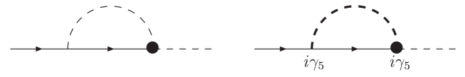
Figure 6: Non-tadpole contributions to $\langle R^{(2)}A\rangle^{(0)}$. The blob denotes the insertion of the operator $D_{2}$ acting on the three legs outgoing from the vertex as in equation (40).

4.1 Calculation in momentum space

In order to verify the WTi (32) we find convenient to work in the momentum space representation.

For the fermion two-point function, the sum of the two diagrams in (35) gives

$$\langle\chi(p)\bar{\chi}(q)\rangle^{(2)}=4g^{2}(2\pi)^{4}\delta^{4}(p+q)\bigg{(}D_{2}(p)-m(1-\frac{a}{2}D_{1}(p))\bigg{)}\int_{k}{\cal G}^{-1}(p,k)D_{2}(p+k)$$

$$\phantom{\langle\chi(p)\bar{\chi}(q)\rangle^{(2)}=\frac{g^{2}}{4}(2\pi)^{4}\delta^{4}(p+q)}\times\bigg{(}D_{2}(p)-m(1-\frac{a}{2}D_{1}(p))\bigg{)}\,,$$ (41)

where

$${\cal G}(p,k)=\big{[}{\cal M}(p)((1-\frac{a}{2}D_{1}(p))\big{]}^{2}\big{[}{\cal M}(k)((1-\frac{a}{2}D_{1}(k))\big{]}\big{[}{\cal M}(k+p)((1-\frac{a}{2}D_{1}(k+p))\big{]}$$ (42)

and $D_{1}(p)$, $D_{2}(p)$ and ${\cal M}(p)$ are the Fourier transform of the operators given in (12) and (16).

Similarly, the terms in (4) and (4) in momentum space write

$$\langle D_{2}(p)(A(p)-i\gamma_{5}B(p))A(q)\rangle^{(2)}=\langle D_{2}(p)A(p)A(q)\rangle^{(2)}=g^{2}(2\pi)^{4}\delta^{4}(p+q)D_{2}(p)$$

$$\phantom{D_{2}(p)}\times\int_{k}{\cal G}^{-1}(p,k)\Big{[}2m^{2}(1-\frac{a}{2}D_{1}(p))^{2}-\mbox{Tr}\big{[}D_{2}(k)D_{2}(p+k)\big{]}+4D_{2}^{2}(k)\Big{]}$$ (43)

and

$$\langle(F(p)-i\gamma_{5}G(p))A(q)\rangle^{(2)}=\langle F(p)A(q)\rangle^{(2)}=mg^{2}(2\pi)^{4}\delta^{4}(p+q)(1-\frac{a}{2}D_{1}(p))$$

$$\phantom{\langle(F(p)-i\gamma_{5}G(p))}\times\int_{k}{\cal G}^{-1}(p,k)\Big{[}\mbox{Tr}\bigg{(}D_{2}(k)D_{2}(p+k)\bigg{)}-4D_{2}^{2}(k)-2D_{2}^{2}(p)\Big{]}\,,$$ (44)

respectively.

Finally, the two terms in (39) and (40) involving $R$ in momentum space become

$$\langle R^{(1)}(p)A(q)\rangle^{(1)}=2mg^{2}(2\pi)^{4}\delta^{4}(p+q)(1-\frac{a}{2}D_{1}(p))\bigg{(}D_{2}(p)-m(1-\frac{a}{2}D_{1}(p))\bigg{)}$$

$$\phantom{\langle R^{(1)}(p)A(q)\rangle^{(1)}=}\times\int_{k}{\cal G}^{-1}(p,k)\bigg{(}2D_{2}(p+k)-D_{2}(p)\bigg{)}$$ (45)

and

$$\langle R^{(2)}(p)A(q)\rangle^{(0)}=-4g^{2}(2\pi)^{4}\delta^{4}(p+q)\bigg{(}D_{2}(p)-m(1-\frac{a}{2}D_{1}(p))\bigg{)}$$

$$\phantom{\langle R^{(2)}(p)A(q)\rangle^{(0)}=}\times\int_{k}{\cal G}^{-1}(p,k)D_{2}(p+k)\bigg{(}D_{2}(k)+D_{2}(p)-D_{2}(p+k)\bigg{)}\,.$$ (46)

In order to verify that the WTi (32) is exactly satisfied, we find convenient to arrange the various terms according to the powers of $m$.

Inserting (4.1) and (4.1)-(4.1) into the WTi (32) and setting $m=0$ one has

$$4g^{2}(2\pi)^{4}\delta^{4}(p+q)\int_{k}{\cal G}^{-1}(p,k)\Big{[}D_{2}(p)D_{2}(p+k)D_{2}(p)+D_{2}(p)\Big{(}D_{2}(k)\cdot D_{2}(p+k)-D_{2}^{2}(k)\Big{)}$$

$$\phantom{g^{2}(2\pi)^{4}\delta^{4}(p+q)\int_{k}{\cal G}^{-1}(p,k)\Big{[}}-D_{2}(p)D_{2}(p+k)\Big{(}D_{2}(k)+D_{2}(p)-D_{2}(p+k)\Big{)}\Big{]}\,,$$ (47)

where $\mbox{Tr}(\gamma_{\mu}\gamma_{\nu})=4\delta_{\mu\nu}$ has been used. Taking advantage of the invariance of ${\cal G}(p,k)$ under the change of variables $k\to-k-p$, one can replace $D_{2}(p+k)D_{2}(k)$ with $\frac{1}{2}\left\{D_{2}(p+k),D_{2}(k)\right\}=D_{2}(p+k)\cdot D_{2}(k)$ and therefore the integrand exactly vanishes.

The terms proportional to $m$ add up to

$$g^{2}(2\pi)^{4}\delta^{4}(p+q)(1-\frac{a}{2}D_{1}(p))\int_{k}{\cal G}^{-1}(p,k)\Big{[}-4\Big{(}D_{2}(p)D_{2}(p+k)+D_{2}(p+k)D_{2}(p)\Big{)}$$

$$\phantom{g^{2}(2\pi)^{4}\delta^{4}(p+q)}+4D_{2}^{2}(k)+2D_{2}^{2}(p)-4D_{2}(k)\cdot D_{2}(p+k)+D_{2}(p)\Big{(}4D_{2}(p+k)-2D_{2}(p)\Big{)}$$

$$\phantom{g^{2}(2\pi)^{4}\delta^{4}(p+q)}+4D_{2}(p+k)\Big{(}D_{2}(k)+D_{2}(p)-D_{2}(p+k)\Big{)}\Big{]}\,.$$ (48)

Performing the substitution $D_{2}(p+k)D_{2}(k)\to D_{2}(p+k)\cdot D_{2}(k)$ as described above it is easy to check that (48) vanishes.

Finally, the contribution left is the one proportional to $m^{2}$, i.e.

$$g^{2}(2\pi)^{4}\delta^{4}(p+q)(1-\frac{a}{2}D_{1}(p))^{2}\int_{k}{\cal G}^{-1}(p,k)\Big{[}4D_{2}(p+k)-2D_{2}(p)$$

$$\phantom{g^{2}(2\pi)^{4}\delta^{4}(p+q)(1-\frac{a}{2}D_{1}(p))^{2}\int_{k}{\cal G}^{-1}(p,k)}-2(2D_{2}(p+k)-D_{2}(p))\Big{]}$$ (49)

which is trivially zero.

This end up our proof that the WTi (32) is exactly satisfied at finite lattice spacing.

5 Continuum limit

In this section we study the continuum limit of the WTi (32) and discuss the restoration of the continuum supersymmetry in this limit. This will clarify the mechanism of cancellation between the different terms in the WTi and the role of the operator $g\langle R(p)A(q)\rangle^{(2)}$.

Following the notation of Ref. [18], the operator $D$ in (9) can be written as

$$D(p)=\bigg{[}\frac{-i\sum_{\mu}\gamma_{\mu}\sin(p_{\mu}a)}{2[\omega(p)+b(p)]}+\frac{a}{2}\bigg{]}^{-1}$$ (50)

where

$$\omega(p)=\frac{1}{a}\bigg{[}\sum_{\mu}\sin^{2}(p_{\mu}a)+(ab(p))^{2}\bigg{]}^{1/2}$$ (51)

and

$$b(p)=\frac{1}{a}\bigg{[}\sum_{\mu}2\sin^{2}(\frac{p_{\mu}a}{2})-1\bigg{]}\,.$$ (52)

With this notation, the operators $D_{1}$ and $D_{2}$ ($D=D_{1}+D_{2}$) are

$$D_{1}(p)=\frac{\omega(p)+b(p)}{a\omega(p)}$$ (53)

and

$$D_{2}(p)=\frac{i}{a^{2}\omega(p)}\sum_{\mu}\gamma_{\mu}\sin(p_{\mu}a)\,.$$ (54)

Similarly,

$$(1-\frac{a}{2}D_{1})=\frac{\omega-b}{2\omega}$$ (55)

and

$${\cal M}^{-1}(1-\frac{a}{2}D_{1})^{-1}=2\omega a^{2}\bigg{[}4(\omega+b)+a^{2}m^{2}(\omega-b)\bigg{]}^{-1}\,.$$ (56)

Each term in the WTi (32) is a function of the external momenta $p$ and can be written as

$$I(p)=\int\frac{d^{4}k}{(2\pi)^{4}}F(k,p)$$ (57)

where the integration momenta $k\in[-\frac{\pi}{a},\frac{\pi}{a}]$. If the integral (57) is ultraviolet convergent, its continuum limit is obtained substituting the function $F(k,p)$ with its continuum equivalent. Otherwise, if (57) is divergent and contains only massive propagators so that $F(k,p)$ is finite for any set of exceptional momenta, one can use the lattice version of the BPHZ technique [19] by writing

$$I(p)\equiv I^{c}(p)+\,I^{l}(p)\,,$$ (58)

where

$$I^{c}(p)=\int{d^{4}k\over(2\pi)^{4}}\bigg{[}F(k,p)-\sum_{n=0}^{n_{F}}{1\over n!}\,p_{\mu_{1}}\ldots p_{\mu_{n}}\bigg{(}{\partial\over\partial p_{\mu_{1}}}\ldots{\partial\over\partial p_{\mu_{n}}}F(k,p)\bigg{)}_{p=0}\bigg{]}\,,$$ (59)

$$I^{l}(p)=\int{d^{4}k\over(2\pi)^{4}}\sum_{n=0}^{n_{F}}{1\over n!}\,p_{\mu_{1}}\ldots p_{\mu_{n}}\bigg{(}{\partial\over\partial p_{\mu_{1}}}\ldots{\partial\over\partial p_{\mu_{n}}}F(k,p)\bigg{)}_{p=0}$$ (60)

and $n_{F}$ is the degree of divergence of the diagram. $I^{c}(p)$ is ultraviolet finite and therefore its continuum limit can be taken. All the effects of the lattice regularization remain in $I^{l}(p)$, which is simply a polynomial in the external momenta with coefficients given by zero-momentum lattice integrals. In the following, we compute the lattice contributions of the Green functions entering in the WTi (32). Before doing this computation, we comment on their continuum part, such as $I^{c}(p)$, containing the subtracted integrand. Since the subtraction makes the integrals UV finite, the order of the limit of zero lattice spacing and the momentum integral can be interchanged. Applying this procedure to $\langle RA\rangle$ one immediately recognizes that its continuum part vanishes, since the function $R$ vanishes for $a\to 0$. This is also clear due to the presence in (4.1) and (4.1) of the factor $D_{2}(k)+D_{2}(p)-D_{2}(p+k)$ that vanishes in this limit. For this reason one can restrict the analysis of the WTi to their lattice part.

For the fermion two point function (4.1), one has to consider the following integral

$$-\frac{i}{a}\int\frac{d^{4}k}{(2\pi)^{4}}\frac{1}{[(\omega^{\prime}+b^{\prime})_{k}+\frac{a^{2}m^{2}}{4}(\omega^{\prime}-b^{\prime})_{k}]}\frac{\omega^{\prime}_{p+k}}{[(\omega^{\prime}+b^{\prime})_{p+k}+\frac{a^{2}m^{2}}{4}(\omega^{\prime}-b^{\prime})_{p+k}]}\sum_{\mu}\gamma_{\mu}\sin(k_{\mu})$$ (61)

where $k$ has been rescaled to $k\to k/a$ and we have defined

$$\omega^{\prime}_{k}\equiv a\omega(k/a)=\bigg{[}1-4\sum_{\mu}\sin^{4}(\frac{k_{\mu}}{2})+4\bigg{(}\sum_{\mu}\sin^{2}(\frac{k_{\mu}}{2})\bigg{)}^{2}\bigg{]}^{1/2}$$ (62)

and

$$\omega^{\prime}_{p+k}\equiv a\omega(p+k/a)=\bigg{[}1-4\sum_{\mu}\sin^{4}(\frac{(k+ap)_{\mu}}{2})+4\bigg{(}\sum_{\mu}\sin^{2}(\frac{(k+ap)_{\mu}}{2})\bigg{)}^{2}\bigg{]}^{1/2}\,.$$ (63)

Similarly, $b^{\prime}_{k}\equiv ab(k/a)$ and $b^{\prime}_{p+k}\equiv ab(p+k/a)$ and their espressions can be easily read from (52).

The factor $1/a$ in (61) implies a linear UV divergence of this integral which is cured by performing a Taylor expansion in $pa$ up to the first derivative. The first term of the Taylor expansion of (61) is odd in $k$, thus is zero, while the first derivative is

$$\int\frac{d^{4}k}{(2\pi)^{4}}\frac{-i\sum_{\mu}\gamma_{\mu}\sin(k_{\mu})}{[(\omega^{\prime}+b^{\prime})_{k}+\frac{a^{2}m^{2}}{4}(\omega^{\prime}-b^{\prime})_{k}]}\sum_{\rho}p_{\rho}\frac{\partial}{\partial p_{\rho}a}\bigg{[}\frac{\omega^{\prime}_{p+k}}{[(\omega^{\prime}+b^{\prime})_{p+k}+\frac{a^{2}m^{2}}{4}(\omega^{\prime}-b^{\prime})_{p+k}]}\bigg{]}_{p=0}$$ (64)

with

$$\frac{\partial}{\partial p_{\rho}a}\bigg{[}\frac{\omega^{\prime}_{p+k}}{[(\omega^{\prime}+b^{\prime})_{p+k}+\frac{a^{2}m^{2}}{4}(\omega^{\prime}-b^{\prime})_{p+k}]}\bigg{]}_{p=0}=\frac{1}{[(\omega^{\prime}+b^{\prime})_{k}+\frac{a^{2}m^{2}}{4}(\omega^{\prime}-b^{\prime})_{k}]^{2}}$$

$$\times\bigg{(}\frac{2}{\omega^{\prime}_{k}}\sum_{\mu\neq\rho}\sin^{2}(\frac{k_{\mu}}{2})\sin(k_{\rho})(2\sum_{\nu}\sin^{2}(\frac{k_{\nu}}{2})-1)-\omega^{\prime}_{k}\sin(k_{\rho})\bigg{)}$$ (65)

plus terms proportional to $a^{2}m^{2}$ which do not contribute in the limit $a\to 0$. Notice that in the denominator the term proportional to $a^{2}m^{2}$ must be kept in order to ensure the IR finiteness of the integral, since $(\omega^{\prime}+b^{\prime})_{k}\sim k^{2}/2$ for $k\to 0$. Indeed, by substituing this derivative in (64) one sees that the contribution from the last term of (65) produces a $\log(a^{2}m^{2})$ divergence (for $a\to 0$) originating from the $k\to 0$ integration region, while the remaining terms give rise to a finite integral.

Therefore, including the external leg factors, the fermion two point function can be written as 

$$\langle\chi\bar{\chi}\rangle^{(2)}(p)=\frac{(i\not p-m)}{(p^{2}+m^{2})}C_{2}i\not p\frac{(i\not p-m)}{(p^{2}+m^{2})}$$ (66)

where

$$C_{2}=g^{2}\int\frac{d^{4}k}{(2\pi)^{4}}\frac{\omega^{\prime}_{k}\sin^{2}(k_{\rho})}{[(\omega+b)^{\prime}_{k}+\frac{a^{2}m^{2}}{4}(\omega-b)^{\prime}_{k}]^{3}}+C_{2f}$$ (67)

and $C_{2f}$ is a finite constant that, for our purposes, need not to be computed.

For the scalar two point function (4.1) one has to calculate the following integral

$$\int\frac{d^{4}k}{(2\pi)^{4}}\bigg{\{}\frac{m^{2}}{2}\frac{\omega^{\prime}_{k}}{[(\omega^{\prime}+b^{\prime})_{k}+\frac{a^{2}m^{2}}{4}(\omega^{\prime}-b^{\prime})_{k}]}\frac{\omega^{\prime}_{p+k}}{[(\omega^{\prime}+b^{\prime})_{p+k}+\frac{a^{2}m^{2}}{4}(\omega^{\prime}-b^{\prime})_{p+k}]}$$

$$\phantom{\int\frac{d^{4}k}{(2\pi)^{4}}\bigg{\{}}-\frac{1}{a^{2}}\frac{1}{(\omega^{\prime}+b^{\prime})_{k}+\frac{a^{2}m^{2}}{4}(\omega^{\prime}-b^{\prime})_{k}}\frac{\omega^{\prime}_{p+k}}{(\omega^{\prime}+b^{\prime})_{p+k}+\frac{a^{2}m^{2}}{4}(\omega^{\prime}-b^{\prime})_{p+k}}$$

$$\phantom{\int\frac{d^{4}k}{(2\pi)^{4}}\bigg{\{}-\frac{1}{a^{2}}}\times\bigg{(}\frac{\sum_{\mu}\sin^{2}(k_{\mu})}{\omega^{\prime}_{k}}-\frac{\sum_{\mu}\sin(k_{\mu})\sin(k_{\mu}+ap_{\mu})}{\omega^{\prime}_{p+k}}\bigg{)}\bigg{\}}\,.$$ (68)

The first term can be evaluated directly at $pa=0$ while for the second we need a Taylor expansion up to the second derivative in $pa$ due to the factor $1/a^{2}$. We first concentrate on the latter term. It vanishes at $pa=0$ and moreover its first derivative is odd in $k$ and therefore also this term of the expansion vanishes. Thus the scalar two point function is given in terms of the following integral

$$\int\frac{d^{4}k}{(2\pi)^{4}}\bigg{\{}\frac{m^{2}}{2}\frac{(\omega^{\prime}_{k})^{2}}{[(\omega^{\prime}+b^{\prime})_{k}+\frac{a^{2}m^{2}}{4}(\omega^{\prime}-b^{\prime})_{k}]^{2}}$$

$$-\frac{1}{(\omega^{\prime}+b^{\prime})_{k}+\frac{a^{2}m^{2}}{4}(\omega^{\prime}-b^{\prime})_{k}}\frac{1}{2}\sum_{\rho\sigma}p_{\rho}p_{\sigma}\frac{\partial^{2}}{\partial p_{\rho}a\partial p_{\sigma}a}\bigg{[}\frac{\omega^{\prime}_{p+k}}{(\omega^{\prime}+b^{\prime})_{p+k}+\frac{a^{2}m^{2}}{4}(\omega^{\prime}-b^{\prime})_{p+k}}$$

$$\phantom{\frac{1}{(\omega^{\prime}+b^{\prime})_{k}+\frac{a^{2}m^{2}}{4}(\omega^{\prime}-b^{\prime})_{k}}}\times\bigg{(}\frac{\sum_{\mu}\sin^{2}(k_{\mu})}{\omega^{\prime}_{k}}-\frac{\sum_{\mu}\sin(k_{\mu})\sin(k_{\mu}+ap_{\mu})}{\omega^{\prime}_{p+k}}\bigg{)}\bigg{]}_{p=0}\bigg{\}}\,.$$ (69)

There are two contributions coming from the second derivative. One is given by the product of (65) with

$$\frac{\partial}{\partial p_{\sigma}a}\frac{\sum_{\mu}\sin(k_{\mu})\sin(k_{\mu}+ap_{\mu})}{\omega^{\prime}_{p+k}}\bigg{|}_{p=0}=\frac{\sin(k_{\sigma})\cos(k_{\sigma})}{\omega^{\prime}_{k}}$$

$$\phantom{\frac{\partial}{\partial p_{\rho}a}\frac{\sum_{\mu}\sin(k_{\mu})\sin(k_{\mu}+ap_{\mu})}{\omega^{\prime}_{p+k}}\bigg{|}_{p=0}}-\frac{2\sum_{\mu}\sin^{2}(k_{\mu})\sum_{\nu\neq\sigma}\sin^{2}(\frac{k_{\nu}}{2})\sin(k_{\sigma})}{(\omega^{\prime}_{k})^{3}}\,,$$ (70)

which produces a $\log(a^{2}m^{2})$ divergence to (69), originating from the product of the last term of (65) with the first term of (70). The second is given by the second derivative of the third line of (69) and its explicit expression is not needed since its contribution to the integral (69) is finite for $a\to 0$.

Collecting all terms and including the external leg factors, the two point function (4.1) becomes

$$D_{2}\langle AA\rangle^{(2)}(p)=i\not p\frac{1}{(p^{2}+m^{2})}\frac{1}{(p^{2}+m^{2})}(\frac{1}{2}C_{3}m^{2}-C_{1}p^{2})$$ (71)

where

$$C_{3}=g^{2}\int\frac{d^{4}k}{(2\pi)^{4}}\frac{(\omega^{\prime}_{k})^{2}}{[(\omega^{\prime}+b^{\prime})_{k}+\frac{a^{2}m^{2}}{4}(\omega^{\prime}-b^{\prime})_{k}]^{2}}\,,$$ (72)

$$C_{1}=g^{2}\int\frac{d^{4}k}{(2\pi)^{4}}\frac{\sin^{2}(k_{\rho})\cos(k_{\rho})}{[(\omega^{\prime}+b^{\prime})_{k}+\frac{a^{2}m^{2}}{4}(\omega^{\prime}-b^{\prime})_{k}]^{3}}+C_{1f}$$ (73)

and $C_{1f}$ is a finite constant.

A similar analysis applied to (4.1) and gives

$$\langle FA\rangle^{(2)}(p)=m\frac{1}{(p^{2}+m^{2})}\frac{1}{(p^{2}+m^{2})}(\frac{1}{2}C_{3}+C_{1})p^{2}\,.$$ (74)

The continuum limit of the two point function containing the operator $R$ can also be determined. For (4.1) and (4.1) one has

$$\langle R^{(1)}A\rangle^{(1)}(p)=m\frac{(i\not p-m)}{(p^{2}+m^{2})}\frac{1}{(p^{2}+m^{2})}(C_{2}-\frac{1}{2}C_{3})i\not p$$ (75)

and

$$\langle R^{(2)}A\rangle^{(0)}(p)=\frac{(i\not p-m)}{(p^{2}+m^{2})}\frac{1}{(p^{2}+m^{2})}(C_{2}-C_{1})p^{2}\,,$$ (76)

respectively. Notice that the combinations $C_{2}-C_{1}$ and $C_{2}-\frac{1}{2}C_{3}$ are two (different) finite numbers. Indeed, looking at the $k\to 0$ behavior of the integrand of (67), (72) and (73) one sees that the $\log(a^{2}m^{2})$ contributions cancels out in these combinations. This is a consequence of the fact that the one-loop correction to the two-point functions of $A$, $F$ and $\chi$ have the same logarithmic divergent parts [20].

Substituting (66), (71) and (74)-(76) in (32) one verifies this WTi in the continuum limit:

$$\frac{(i\not p-m)}{(p^{2}+m^{2})}(i\not pC_{2})\frac{(i\not p-m)}{(p^{2}+m^{2})}$$

$$-\frac{i\not p}{(p^{2}+m^{2})}(\frac{1}{2}m^{2}C_{3}-p^{2}C_{1})\frac{1}{(p^{2}+m^{2})}$$

$$-\frac{m}{(p^{2}+m^{2})}(C_{1}+\frac{1}{2}C_{3})p^{2}\frac{1}{(p^{2}+m^{2})}$$

$$+\frac{(i\not p-m)}{(p^{2}+m^{2})}(i\not pm)(C_{2}-\frac{1}{2}C_{3})\frac{1}{(p^{2}+m^{2})}$$

$$+\frac{(i\not p-m)}{(p^{2}+m^{2})}(C_{2}-C_{1})p^{2}\frac{1}{(p^{2}+m^{2})}=0\,.$$ (77)

Actually, this is a check of the results we have obtained for the continuum limit of the two point functions, since we have proved that this WTi holds for any $a$ and therefore must be verified also in the limit $a\to 0$. Notice that the term $\langle RA\rangle$ in (31) is essential to recover the WTi (32) also for $a\to 0$.

Let us clarify the role of the operator $R$. Thanks to the exactness of WTi (32) it is always possible to write the two point function $\langle RA\rangle^{(2)}$ as a suitable combination of the other three two point functions involved in this WTi. In particular, in the continuum limit one can write

$$\langle RA\rangle=\frac{i\not p-m}{p^{2}+m^{2}}i\not p\delta_{1}\frac{i\not p-m}{p^{2}+m^{2}}+i\not p\frac{1}{p^{2}+m^{2}}(\delta_{2}p^{2}+\delta_{3}m^{2})\frac{1}{p^{2}+m^{2}}$$

$$\phantom{\langle RA\rangle=}-\frac{m}{p^{2}+m^{2}}(\delta_{2}-\delta_{3})p^{2}\frac{1}{p^{2}+m^{2}}$$ (78)

where, from (75) and (76),

$$\delta_{1}=\frac{1}{2}C_{3}-C_{2}-\delta_{3}\,,\;\;\;\;\;\;\;\delta_{2}=\frac{1}{2}C_{3}-C_{1}-\delta_{3}\,,\;\;\;\;\;\;\;$$ (79)

and the constant $\delta_{3}$ is arbitrary. Then in the continumm limit one can rewrite the WTi (32) as the supersymmetric continuum WTi

$$\langle\chi\bar{\chi}\rangle_{R}^{(2)}-i\not p\langle AA\rangle_{R}^{(2)}-\langle FA\rangle_{R}^{(2)}=0$$ (80)

with

$$\langle\chi\bar{\chi}\rangle_{R}^{(2)}\equiv\langle\chi\bar{\chi}\rangle^{(2)}+\frac{i\not p-m}{p^{2}+m^{2}}i\not p\delta_{1}\frac{i\not p-m}{p^{2}+m^{2}}$$

$$\langle AA\rangle_{R}^{(2)}\equiv\langle AA\rangle_{(2)}-\frac{1}{p^{2}+m^{2}}(\delta_{2}p^{2}+\delta_{3}m^{2})\frac{1}{p^{2}+m^{2}}$$

$$\langle FA\rangle_{R}^{(2)}\equiv\langle FA\rangle^{(2)}+\frac{m}{p^{2}+m^{2}}(\delta_{2}-\delta_{3})p^{2}\frac{1}{p^{2}+m^{2}}$$ (81)

It is convenient to express these two point functions in terms of 1PI vertex functions:

$$\langle\chi\bar{\chi}\rangle^{(2)}=\frac{i\not p-m}{p^{2}+m^{2}}\,\Sigma^{(2)}_{\chi\bar{\chi}}\,\frac{i\not p-m}{p^{2}+m^{2}}\,,$$

$$\langle AA\rangle^{(2)}=-\frac{1}{p^{2}+m^{2}}(\Sigma^{(2)}_{AA}+m^{2}\Sigma^{(2)}_{FF})\frac{1}{p^{2}+m^{2}}\,,$$

$$\langle FA\rangle^{(2)}=\frac{1}{p^{2}+m^{2}}(\Sigma^{(2)}_{AA}-p^{2}\Sigma^{(2)}_{FF})\frac{m}{p^{2}+m^{2}}\,,$$ (82)

where the vanishing of the 1PI $AF$-vertex has been used. ¿From (66), (71) and (74), the lattice contribution to these 1PI vertices in the continuum limit reads

$$\Sigma^{(2)}_{\chi\bar{\chi}}=i\not pC_{2}\,,\;\;\;\;\;\;\;\Sigma^{(2)}_{AA}=p^{2}C_{1}\,,\;\;\;\;\;\;\;\Sigma^{(2)}_{FF}=-\frac{1}{2}C_{3}\,.$$ (83)

Moreover, from (81), one has

$$\Sigma^{(2)}_{\chi\bar{\chi}\,R}\equiv\Sigma^{(2)}_{\chi\bar{\chi}}+i\not p\delta_{1}=i\not p(\frac{C_{3}}{2}-\delta_{3})\equiv-Z_{\chi}i\not p$$

$$\Sigma^{(2)}_{AA\,R}\equiv\Sigma^{(2)}_{AA}+p^{2}\delta_{2}=p^{2}(\frac{C_{3}}{2}-\delta_{3})\equiv-Z_{A}p^{2}$$

$$\Sigma^{(2)}_{FF\,R}\equiv\Sigma^{(2)}_{FF}+\delta_{3}=-(\frac{C_{3}}{2}-\delta_{3})\equiv Z_{F}$$ (84)

with

$$Z_{\chi}=Z_{A}=Z_{F}=-(\frac{C_{3}}{2}-\delta_{3})\,.$$ (85)

In Ref. [20] it was shown that the one-loop corrections to the two-point function of $A$, $F$ and $\chi$ differ by finite quantities. Our construction shows that if one redefines the 1PI vertices as in (84) the wave function renormalization factors become equal. This is an important consequence of the exact lattice supersymmetry we have introduced and of the WTi derived from this symmetry. This automatically leads to restoration of supersymmetry in the continuum limit with equal renormalization wave function for the scalar and fermion fields.

In a more standard approach [12, 21] the function $R$ is not included in the lattice supersymmetry transformation. Since the action is not invariant under this transformation, the WTi contains a breaking term. From the $a\to 0$ limit of this WTi one determines the counterterms nedeed to restore supersymmetry in the continuum limit. The central issue of our approch is that this possibility is guaranteed by the existence of an exact supersymmetry of the lattice action.

6 Conclusions

In this paper, starting from the $N=1$ four dimensional lattice Wess-Zumino model that uses the Ginsparg-Wilson relation and keeps an exact supersymmetry on the lattice, it is showed that the corresponding Ward-Takahashi identity is satisfied, both at fixed lattice spacing and in the continuum limit. This result crucially depends on the Ginsparg-Wilson properties of the operators involved in the lattice action. The calculation is performed in lattice perturbation theory up to order $g^{2}$ in the coupling constant.

It is also showed that the study of the continuum limit of this Ward-Takahashi identity determines the finite part of the scalar and fermion renormalization wave functions which automatically leads to restoration of supersymmetry in the continuum limit. In particular, these wave functions coincide in this limit.

Although we limit our computation up to the order $g^{2}$, this order is not trivial and the discussion is general and applies to higher orders by following the procedure described in this work.

There are several issues that remain to be investigated. First of all it will be interesting to perform numerical simulations of this model to check non-perturbatively the WTi (31). Furthermore, one of the most important question is whether these ideas may be extended to theories with a gauge symmetry.

Acknowledgements
A.F. would like to thank Mike Creutz, John Kogut, Herbert Neuberger and Tilo Wettig for organizing the program “Modern Challenges in Lattice Field Theory” at KITP where part of this work was completed. This research was supported in part by the National Science Foundation under Grant No. PHY99-07949.

7 Appendix A

The fermionic kinetic term in the action (2),

$$(1-\frac{a}{2}D_{1})^{-1}D_{2}$$ (86)

needs a careful study at the border of the Brillouin zone. To this end we set

$$p_{\mu}=(0,0,0,\frac{\pi-\epsilon}{a})$$ (87)

and study the limit $\epsilon\to 0$. Using Eqs. (51) and (52) we have that

$$b=\frac{1}{a}\big{[}1-\frac{\epsilon^{2}}{2}+{\cal O}(\epsilon^{4})\big{]}$$ (88)

and

$$\omega=\frac{1}{a}\,.$$ (89)

Inserting these values in (54) and (55) we find

$$(1-\frac{a}{2}D_{1})^{-1}=\frac{4}{\epsilon^{2}}\big{[}1+{\cal O}(\epsilon^{2})\big{]}$$ (90)

and

$$D_{2}=i\gamma_{4}\frac{\epsilon}{a}\big{[}1+{\cal O}(\epsilon^{2})\big{]}\,.$$ (91)

Finally, the fermionic kinetic operator (86) behaves as

$$(1-\frac{a}{2}D_{1})^{-1}D_{2}=4i\gamma_{4}\frac{1}{a\epsilon}\big{[}1+{\cal O}(\epsilon^{2})\big{]}$$ (92)

thus in the limit $\epsilon\to 0$ with fixed $a$ the would be doubler (87) becomes (infinitely) massive. Similarly, one can check that this value of the momentum do not generate a pole in the bosonic propagators. This analysis can be generalized to the other edges of the Brillouin zone. For instance, if

$$p_{\mu}=(0,0,\frac{\pi-\epsilon}{a},\frac{\pi-\epsilon}{a})$$ (93)

we have

$$(1-\frac{a}{2}D_{1})^{-1}D_{2}=i(\gamma_{3}+\gamma_{4})\frac{3}{a\epsilon}$$ (94)

which again becomes a massive mode when $\epsilon\to 0$ while $a$ is kept fixed. It is easy to demostrate that all the rest of the would be zero modes behave in the same way.

Notice that the fermion propagator in (2) can be rewritten as

$$\langle\chi\bar{\chi}\rangle=-(D_{2}-m(1-\frac{a}{2}D_{1}))\,\Big{[}\frac{2}{a}D_{1}+m^{2}(1-\frac{a}{2}D_{1})\Big{]}^{-1}$$ (95)

which is clearly finite for $\epsilon\to 0$.

Appendix B

In this appendix we explicitly show that the tadpole contributions to the two point WTi (32) cancel separately. For the $\langle\bar{\chi}_{y}\chi_{x}\rangle^{(2)}$ two point function this has been already shown in Section 5.
The tadpole contribution to $\langle D_{2yz}(A_{z}-i\gamma_{5}B_{z})A_{x}\rangle$ is

$$\langle D_{2yz}(A_{z}-i\gamma_{5}B_{z})A_{x}\rangle^{(2)}_{T}=g^{2}\Big{\{}D_{2yz}\langle A_{z}A_{u}\rangle\Big{[}\langle F_{u}A_{w}\rangle\Big{(}2\langle F_{w}A_{w}\rangle+2\langle G_{w}B_{w}\rangle-\mbox{Tr}\langle\chi_{w}\bar{\chi}_{w}\rangle\Big{)}$$

$$\phantom{\langle D_{2yz}(A_{z}-i\gamma_{5}B_{z})A_{x}\rangle^{(2)}_{T}=g^{2}D_{2yz}\langle A_{z}A_{u}\rangle\Big{]}}+\langle F_{u}F_{w}\rangle\Big{(}\langle A_{w}A_{w}\rangle-\langle B_{w}B_{w}\rangle\Big{)}\Big{]}\langle A_{u}A_{x}\rangle$$

$$\phantom{\langle D_{2yz}(A_{z}-i\gamma_{5}B_{z})A_{x}\rangle^{(2)}_{T}}+D_{2yz}\langle A_{z}F_{u}\rangle\Big{[}\langle A_{u}A_{w}\rangle\Big{(}2\langle F_{w}A_{w}\rangle+2\langle G_{w}B_{w}\rangle-\mbox{Tr}\langle\chi_{w}\bar{\chi}_{w}\rangle\Big{)}$$

$$\phantom{\langle D_{2yz}(A_{z}-i\gamma_{5}B_{z})A_{x}\rangle^{(2)}_{T}=D_{2yz}\langle A_{z}A_{u}\rangle}+\langle A_{u}F_{w}\rangle\Big{(}\langle A_{w}A_{w}\rangle-\langle B_{w}B_{w}\rangle\Big{)}\Big{]}\langle A_{u}A_{x}\rangle$$

$$\phantom{\langle D_{2yz}(A_{z}-i\gamma_{5}B_{z})A_{x}\rangle^{(2)}_{T}}+D_{2yz}\langle A_{z}A_{u}\rangle\Big{[}\langle A_{u}A_{w}\rangle\Big{(}2\langle F_{w}A_{w}\rangle+2\langle G_{w}B_{w}\rangle-\mbox{Tr}\langle\chi_{w}\bar{\chi}_{w}\rangle\Big{)}$$

$$\phantom{\langle D_{2yz}(A_{z}-i\gamma_{5}B_{z})A_{x}\rangle^{(2)}_{T}=D_{2yz}\langle A_{z}A_{u}\rangle}+\langle A_{u}F_{w}\rangle\Big{(}\langle A_{w}A_{w}\rangle-\langle B_{w}B_{w}\rangle\Big{)}\Big{]}\langle F_{u}A_{x}\rangle\Big{\}}\,.$$ (96)

Similarly, the tadpole contribution to $\langle(F_{y}-i\gamma_{5}G_{y})A_{x}\rangle$ is

$$\langle(F_{y}-i\gamma_{5}G_{y})A_{x}\rangle^{(2)}_{T}=\langle F_{y}A_{u}\rangle\Big{[}\langle F_{u}A_{w}\rangle\Big{(}2\langle F_{w}A_{w}\rangle+2\langle G_{w}B_{w}\rangle-\mbox{Tr}\langle\chi_{w}\bar{\chi}_{w}\rangle\Big{)}\\ +\langle A_{u}F_{w}\rangle\Big{(}\langle A_{w}A_{w}\rangle-\langle B_{w}B_{w}\rangle\Big{)}\Big{]}\langle A_{u}A_{x}\rangle\\ +\langle F_{y}F_{u}\rangle\langle A_{u}A_{w}\rangle\Big{[}2\langle F_{w}A_{w}\rangle+2\langle G_{w}B_{w}\rangle-\mbox{Tr}\langle\chi_{w}\bar{\chi}_{w}\rangle\Big{]}\langle A_{u}A_{x}\rangle\,.$$ (97)

It is easy to see that both expressions are exactly zero.

References

[1] P. H. Dondi and H. Nicolai, Nuovo Cim. A41 (1977) 1.
[2] S. Elitzur, E. Rabinovici, A. Schwimmer, Phys. Lett. B119 (1982) 165;
J. Bartels and G. Kramer, Z. Phys. C20 (1983) 159;
T. Banks and P. Windey, Nucl. Phys. B198 (1982) 226;
J. Bartels and J. B. Bronzan, Phys. Rev. D28 (1983) 818;
M. F. L. Golterman and D. N. Petcher, Nucl. Phys. B319 (1989) 307;
W. Bietenholz, Mod. Phys. Lett. A14 (1999) 51;
S. Catterall, S. Karamov, Phys. Rev. D68 (2003) 014503;
M. Beccaria, M. Campostrini, A. Feo, Phys. Rev. D69 (2004) 095010;
M. Beccaria, M. Campostrini, G. F. De Angelis, A. Feo, Phys. Rev. D70 (2004) 035011.
[3] G. Curci and G. Veneziano, Nucl. Phys. B292 (1987) 555.
[4] D. B. Kaplan, Nucl. Phys. Proc. Suppl. 129 (2004) 109;
A. Feo, Nucl. Phys. Proc. Suppl. 119 (2003) 198;
A. Feo, Mod. Phys. Lett. A19 (2004) 2387.
[5] I. Montvay, Nucl. Phys. B466 (1996) 259;
I. Montvay, Int. J. Mod. Phys. A17 (2002) 2377 (and references therein).
[6] D. B. Kaplan, E. Katz, M. Unsal, JHEP 0305 (2003) 037;
A. G. Cohen, D. B. Kaplan, E. Katz, M. Unsal, JHEP 0308 (2003) 024;
A. G. Cohen, D. B. Kaplan, E. Katz, M. Unsal, JHEP 0312 (2003) 031;
[7] J. Nishimura, S. Rey, F. Sugino, JHEP 0302 (2003) 032.
[8] S. Catterall, JHEP 0305 (2003) 038;
S. Catterall and S. Ghadab, JHEP 0405 (2004) 044;
[9] F. Sugino, JHEP 0403 (2004) 067;
F. Sugino, JHEP 0501 (2005) 016.
[10] A. D’Adda, I. Kanamori, N. Kawamoto, K. Nagata, Nucl. Phys. B707 (2005) 100.
[11] S. Catterall, hep-lat/0503036.
[12] K. Fujikawa, Nucl. Phys. B636 (2002) 80.
[13] K. Fujikawa and M. Ishibashi, Phys. Lett. B528 (2002) 295.
[14] M. Bonini and A. Feo, JHEP 0409 (2004) 011;
M. Bonini and A. Feo, hep-lat/0409068.
[15] P. H. Ginsparg and K. G. Wilson, Phys. Rev. D25 (1982) 2649.
[16] M. Lüscher, Phys. Lett. B428 (1998) 342;
P. Hernandez, K. Jansen, M. Lüscher, Nucl. Phys. B552 (1999) 363.
[17] H. Neuberger, Phys. Lett. B417 (1998) 141;
H. Neuberger, Phys. Lett. B427 (1998) 353.
[18] Y. Kikukawa and A. Yamada, Phys. Lett. B448 (1999) 265.
[19] T. Reisz, Commun. Math. Phys. 116 573 (1988);
T. Reisz, Commun. Math. Phys. 116 81 (1988).
[20] K. Fujikawa and M. Ishibashi, Nucl. Phys. B622 (2002) 115.
[21] Y. Kikukawa and H. Suzuki, JHEP 0502 (2005) 012.