More on the finite size mass shift formula for stable particles

Abstract

The next to leading order (NLO) contribution of the generalized finite size mass shift formula for an interacting two stable particle system in a periodic $L^{3}$ box is discriminated with maintaining its model independent structure and validity to all orders in perturbation theory. The influence of the NLO contribution is examined for the nucleon mass shift in the realistic nucleon-pion system.

Measurements of hadron spectrum in unquenched lattice QCD simulations always suffer the finite volume effect from the associated virtual cloud of lightest particles in the spectra, which may lap the whole lattice once or several times owing to periodic boundary conditions. Finite size mass shift formulae, involving the quantum loop effect of pions in finite volume, are thus derived in chiral perturbation theory (ChPT) [1, 2, 3, 4, 5, 6, 7, 8] and applied to the simulation results for the purpose of controlling its volume dependence and of identifying the value corresponding to the thermodynamic limit (see [9] for a recent review).

In our previous paper, we looked at this issue [10] from a general field theoretical point of view (without sticking to ChPT) and derived the finite size mass shift formula for the interacting two stable particle system in a periodic $L^{3}$ box, as an extension of Lüscher’s formula for self-interacting bosons [11, 12]. Remarkable points of Lüscher’s formula are that the finite size mass shift in a periodic box is related to forward elastic scattering amplitudes in infinite volume, which is model independent, and can be valid to all orders in perturbation theory up to a certain error term [12].

In perturbation theory the physical mass is defined from the pole position of the full propagator. Using this fact, the finite size mass shift of a (bosonic) particle  $\Delta m(L)=M(L)-m$ in Euclidean space can be defined as

$$\Delta m(L)=-\frac{1}{2m}[\Sigma_{L}(p)-\Sigma(p)]+O((\Delta m)^{2})\quad\mbox{at}\quad p=(im,\vec{0}\,)\;,$$ (1)

where $\Sigma_{L}(p)$ and $\Sigma(p)$ denote the self energies in the finite and infinite volumes, respectively. We renormalize the self energy in infinite volume as $\Sigma(p)=\frac{\partial}{\partial p^{2}}\Sigma(p)=0$ at $p^{2}=-m^{2}$. In perturbation theory $\Sigma_{L}(p)$ contains the number of sums over discrete spatial loop momenta, $\vec{q}_{i}(L)=2\pi\vec{n}_{i}/L$ $(\vec{n}_{i}\in\mathbb{Z}^{3})$, depending on the number of loops ($i=1,\ldots,N_{\rm loop}$). These summations can be rewritten as integrals by using the Poisson summation formula. Then the integrand of $\Sigma_{L}(p)$ is reduced to the same form as that of $\Sigma(p)$ apart from the exponential factors $e^{-iL\vec{m}_{i}\cdot\vec{q}_{i}}$ and summations over integer vectors $\vec{m}_{i}\in\mathbb{Z}^{3}$.

Since the magnitude of $\vec{m}_{i}\in\mathbb{Z}^{3}$ acts as the weight of the exponential suppression factor of the mass shift formula, the leading order (LO) contribution to $\Delta m(L)$ for an asymptotically large $L$ can be specified by requiring that only one of them has a non-zero value $|\vec{m}|\equiv|\vec{m}_{i}|=1$ and the others have zero $|\vec{m}_{j}|=0$ ($j\neq i$). In other words, the asymptotic formula can be described by the collection of the effective one-loop diagrams with an exponential factor $e^{-iL\vec{m}\cdot\vec{q}}$, where the other loop integrals without exponential factors are reduced to the part of the definition of the vertex function in infinite volume. Lüscher originally discussed this case [11, 12] and we also did it in the previous paper [10]. The order of the error term in the formula was then consistent with that of the next to leading order (NLO) contribution; $|\vec{m}|=|\vec{m}_{i}|=\sqrt{2}$ and $|\vec{m}_{j}|=0$ ($j\neq i$).

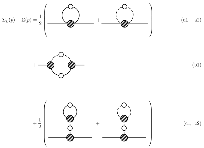
Figure 1: Effective one-loop self-energy diagrams which contribute to the mass shift formula in the bosonic $A$-$B$ system. Solid lines with an empty circle correspond to the propagator of $A$ particle, $G_{A}$, and dashed lines to that of $B$ particle, $G_{B}$. Shaded blobs are vertex functions, $\Gamma_{AAB}$, $\Gamma_{AAAA}$, $\Gamma_{AABB}$, $\Gamma_{BBB}$, at certain orders in perturbation theory. It is assumed that $A$ particle carries a conserved charge.

For the realistic application of the formula to analyzing lattice data, however, it is desirable to reduce the ambiguity associated with the error term. In the present paper, we thus aim to discriminate the NLO contribution ($|\vec{m}|=\sqrt{2}$) in the formula for the two particle ($A$-$B$) system, in particular, while maintaining its model independent structure and validity to all orders in perturbation theory. In this case, the task is still the same as for the $|\vec{m}|=1$ case; we evaluate the effective one-loop diagrams as listed in Fig. 1. We may here assume that $A$ particle carries a conserved charge, so that interaction induced by the three-point vertex $AAB$ and four-point charge conserving vertices are taken into account. It should be noted that what is nontrivial for such an extension is not so much evaluating the $|\vec{m}|=\sqrt{2}$ contribution itself as evaluating the $|\vec{m}|=1$ contribution with an error term at most of the order of the NNLO contribution ($|\vec{m}|=\sqrt{3}$). Otherwise the NLO contribution will be obscured in the error term. In fact, it is straightforward to compute the $|\vec{m}|=\sqrt{2}$ contribution once the procedure is established for $|\vec{m}|=1$.

The result turns out that for the mass ratio

$$\alpha\equiv\frac{m_{B}}{m_{A}}\in(0,\alpha_{\rm max}]$$ (2)

with $\alpha_{\rm max}\approx 0.418$, it is possible to discriminate the NLO contribution and the final expression can be written as

$$\Delta m_{A}(L) = -\frac{1}{16\pi m_{A}}\left(\frac{6}{L}\right)\Biggl{[}\frac{\lambda^{2}}{2\nu_{B}}e^{-L\mu}+\int_{-\infty}^{\infty}\frac{dq_{0}}{2\pi}e^{-L\sqrt{q_{0}^{2}+m_{B}^{2}}}F_{AB}(iq_{0})\Biggr{]}$$ (3)

$$-\frac{1}{16\pi m_{A}}\left(\frac{12}{\sqrt{2}L}\right)\Biggl{[}\frac{\lambda^{2}}{2\nu_{B}}e^{-\sqrt{2}L\mu}+\int_{-\infty}^{\infty}\frac{dq_{0}}{2\pi}e^{-\sqrt{2}L\sqrt{q_{0}^{2}+m_{B}^{2}}}F_{AB}(iq_{0})\Biggr{]}$$

$$+O(e^{-\sqrt{3}L\mu})\;,$$

where the first and second lines correspond to the LO and NLO contributions, respectively. In this expression,

$$\mu\equiv m_{B}\sqrt{1-\frac{\alpha^{2}}{4}}=\sqrt{m_{B}^{2}-\nu_{B}^{2}},\qquad\nu_{B}=\frac{m_{B}^{2}}{2m_{A}}\;,$$ (4)

and $F_{AB}(\nu)$ denotes the forward scattering amplitude of $A(p)+B(q)\to A(p)+B(q)$ in infinite volume ($\nu=iq_{0}$ the crossing variable). $F_{AB}(\nu)$ has poles at $\nu=\pm\nu_{B}$. The coupling $\lambda$ is then defined by exploiting the residue of $F_{AB}(\nu)$ as

$$\lim_{\nu\to\pm\nu_{B}}(\nu^{2}-\nu_{B}^{2})F_{AB}(\nu)=\frac{\lambda^{2}}{2}\;.$$ (5)

The basic line of the derivation of Eq. (3) is the same as in our previous paper [10], where the detailed notation of the propagators and the vertex functions are also given. In what follows, we shall present a derivation for the case that both $A$ and $B$ particles are bosons. The extension to the case that particle $A$ is a fermion is straightforward, and the final result is exactly the same as in Eq. (3), which is one of the advantages of the model independence of the formula. Here, we concentrate on evaluating the diagram (b1) in Fig. 1, which is typical for the two particle system and provides us with a key idea how to control the error term. The other diagrams are then evaluated in a similar way.

The self-energy diagram (b1) for $|\vec{m}|=1$ is expressed as

$$I_{b1}^{(|\vec{m}|=1)} = 6\int\frac{d^{4}q}{(2\pi)^{4}}e^{iLq_{1}}\Gamma_{\mathit{AAB}}(-p,(1-\eta)p+q;\eta p-q)G_{A}((1-\eta)p+q)$$ (6)

$$\times G_{B}(\eta p-q)\Gamma_{\mathit{AAB}}(p,-(1-\eta)p-q;-\eta p+q)\biggr{|}_{p=(im_{A},\;\vec{0}\,)}\;,$$

where $\eta$ is a real parameter at least in the range $[0,2\delta(\alpha)]$ for $\delta(\alpha)\in(0,1/2]$. For the purposes of evaluating the integral $\eta$ can be chosen appropriately depending on the mass ratio $\alpha$. Our concern is whether there exists such a set of $\eta$ and $\delta$ for a given $\alpha$ to make the error terms smaller than the desired order of magnitude. For our purpose this is $O(e^{-L\gamma\mu})$ with $\gamma=\sqrt{3}$. In our previous work [10], we chose $\eta=\delta=\alpha^{2}/2$, which was sufficient to control the error term up to $O(e^{-\sqrt{2}L\mu})$. But this choice turns out to be inappropriate in the present case (see our final choice in Eq. (12)). The overall factor 6 originates from rotational invariance among $q_{1}$, $q_{2}$ and $q_{3}$.

Firstly, we perform the complex $q_{1}$ contour integration by focusing on the poles of the propagators $G_{A}$ and $G_{B}$ of one-particle states at 

$$q_{1}^{(A)}=i\sqrt{q_{0}^{2}+q_{\perp}^{2}+(2\eta-\eta^{2})m_{A}^{2}+i2(1-\eta)m_{A}q_{0}}\;,$$ (7)

$$q_{1}^{(B)}=i\sqrt{q_{0}^{2}+q_{\perp}^{2}+m_{B}^{2}-\eta^{2}m_{A}^{2}-i2\eta m_{A}q_{0}}\;,$$ (8)

in the complex $q_{1}$ upper half plane, respectively,  where $q_{\perp}^{2}=q_{2}^{2}+q_{3}^{2}$. We may set a contour which goes along the real $q_{1}$ line and the line $\mbox{Im}~{}q_{1}=\theta_{1}>0$ closed at $\pm\infty$ to pick up the residues at $q_{1}^{(A)}$ and/or $q_{1}^{(B)}$. In order to relate the mass shift to the on-shell forward scattering amplitude like in Eq. (3), we find at this point that the upper path $\theta_{1}$ must be chosen so as to satisfy the following conditions;

1. the contribution from the upper path itself is smaller than the error term $O(e^{-L\gamma\mu})$,

2. the contour covers the range of $\mbox{Im}~{}q_{1}^{(A)}$ and/or $\mbox{Im}~{}q_{1}^{(B)}$ for $q_{0}$ and $q_{\perp}$ in a certain ball

   $$\mathbb{B}=\{(q_{0},q_{\perp})\in\mathbb{R}^{3}~{}|~{}q_{0}^{2}+q_{\perp}^{2}\leq\nu^{2}\}\;,$$ (10)

3. the contour picks up no residue except for the poles at $q_{1}^{(A)}$ and/or $q_{1}^{(B)}$.

Here the condition (iii) must be guaranteed even if $q_{0}$ is extended to a complex variable and shifted as $q_{0}\to q_{0}-i(1-\eta)m_{A}$ for $q_{1}^{(A)}$ and/or $q_{0}\to q_{0}+i\eta m_{A}$ for $q_{1}^{(B)}$, where $q$ satisfies the on-shell condition $q^{2}=-m_{A}^{2}$ and/or $q^{2}=-m_{B}^{2}$.

To examine the condition (iii), we use the fact that the vertex function $\Gamma_{\mathit{AAB}}(\mp p,(1-\eta)p\pm q;\eta p\mp q)$ with $\eta\in[0,2\delta]$, initially defined for $(p,q)\in\mathbb{R}^{4}\times\mathbb{R}^{4}$, is analytic inside the complex domain

$$\mathbb{D} = \{(p,q)\in\mathbb{C}^{4}\times\mathbb{C}^{4}~{}|~{}\left(\mathrm{Im}\{(1-\delta)\,p\pm\frac{1}{2}\,q\}\right)^{2}<m_{A}^{2}\;,$$ (11)

$$\qquad\qquad\qquad\qquad\quad\left(\mathrm{Im}\{\delta\,p\pm\frac{1}{2}\,q\}\right)^{2}<m_{B}^{2}\;\}\;.$$

The basic observation for finding this domain is that the vertex function at any higher order in perturbation theory consists of a set of $A$ and $B$ lines (free propagators). The denominator of the $l$th $A$ or $B$ line is then parametrized as $(k(l)+r(l))^{2}+m_{A}^{2}$ or $(k(l)+r(l))^{2}+m_{B}^{2}$, where $k(l)$ is the external momentum flow given by a combination of complex variables $p$ and $q$, and $r(l)$ is a combination of internal loop momenta to be integrated out, which is a real variable in Euclidean space. It then follows that the vertex function has no singularity if $(\mathrm{Im}~{}k(l))^{2}<m_{A}^{2}$ and $(\mathrm{Im}~{}k(l))^{2}<m_{B}^{2}$ for all $A$ and $B$ lines. In order to find the possible choices of $k(l)$, we may label the three bare vertices where the external momenta, $p$, $(1-\eta)p+q$ and $\eta p-q$, are plugged in (and out) as $a_{1}$, $a_{2}$ and $b$, respectively (e.g. $a_{1}=a_{2}=b$ at the tree level). Note that whenever $A$ particle carries a conserved charge, there always exists a set of $A$ lines connecting $a_{1}$ and $a_{2}$. In Fig. 2, we show the possible external momentum flow inside the $AAB$ vertex function; they are basically classified into two cases, the connected $A$ lines flow through $b$ (left) and the connected $A$ lines do not flow through $b$ (right). One can add any internal lines depending on the order in perturbation theory, which however carry no external momentum and do not affect the singularity of the vertex function. Inserting the largest external momenta for $A$ and $B$ lines into $(\mathrm{Im}~{}k(l))^{2}<m_{A}^{2}$ and $(\mathrm{Im}~{}k(l))^{2}<m_{B}^{2}$, respectively, one can specify the domain $\mathbb{D}$ as in (11).

Figure 2: The external momentum flow in the $AAB$ vertex function. Arrows represent the flow direction.

We then realize that there is no integration path $\theta_{1}$ at any value of $\alpha$ which satisfies all conditions (i)$\sim$(iii) for both poles $q_{1}^{(A)}$ and $q_{1}^{(B)}$ simultaneously. However, we find that it is possible to choose $\theta_{1}=\sqrt{\gamma^{2}\mu^{2}+\eta^{2}m_{A}^{2}}$ with the upper bound of the ball $\nu^{2}=\gamma^{2}\mu^{2}-m_{B}^{2}+\eta^{2}m_{A}^{2}$ in Eq (10), which satisfies the conditions only for $q_{1}^{(B)}$ within a limited range of $\alpha$. The choice of $\eta$ and $\delta$ is quite subtle, but by choosing

$$\eta=c\;\delta\;,\qquad\delta=\alpha\sqrt{\frac{4-\gamma^{2}(1-\frac{\alpha^{2}}{4})}{2(c^{2}+2c+2)}}\;.$$ (12)

with $c=0.95$, the allowed range of $\alpha$ is maximized as $\alpha\in(0,\alpha_{\rm max}]$, where $\alpha_{\rm max}\approx 0.418$.  Thus we obtain

$$I_{b1}^{(|\vec{m}|=1)} = 6i\int_{\mathbb{B}}\frac{dq_{0}d^{2}q_{\perp}}{(2\pi)^{3}}\frac{e^{iLq_{1}}}{2q_{1}}\Gamma_{\mathit{AAB}}(-p,(1-\eta)p+q;\eta p-q)$$ (13)

$$\times G_{A}((1-\eta)p+q)\Gamma_{\mathit{AAB}}(p,-(1-\eta)p-q;-\eta p+q)|_{q_{1}=q_{1}^{(B)}}$$

$$+O(e^{-L\gamma\mu})\;.$$

We remark that if we set $\gamma=2$, where $O(e^{-2L\mu})$ corresponds to the NNNLO contribution, there is no parameter set $(\theta_{1},\eta,\delta,\nu)$ which fulfills the above conditions at any value of $\alpha$, indicating that one cannot discriminate the NNLO contributions along this line.

Figure 3: $q_{0}$ integration contour.

Secondly, we perform the complex $q_{0}$ contour integration along the path in Fig. 3. The path $CD$ is parametrized by shifting the momentum $q_{0}\to q_{0}+i\eta m_{A}$. On this path the argument of $G_{A}$ becomes $p+q$, where $q$ satisfies the on-shell condition $q^{2}=-m_{B}^{2}$, since $q_{1}^{(B)}=i\sqrt{q_{0}^{2}+q_{\perp}^{2}+m_{B}^{2}}$. Inside the contour the integrand has no pole except at

$$q_{0}=q_{0}^{\prime}=im_{A}\left(\eta-\frac{\alpha^{2}}{2}\right)\;,$$ (14)

which is guaranteed by the above condition (iii). Note that $0<\mbox{Im}~{}q_{0}^{\prime}<\eta m_{A}$ for the value of $\eta$ specified by Eq. (12). The contributions from the paths $BC$ and $DA$ are at most $O(e^{-L\gamma\mu})$ since $\mbox{Im}~{}q_{1}^{(B)}\geq\gamma\mu$, which is due to the choice of the ball $\mathbb{B}$ with $\nu^{2}=\gamma^{2}\mu^{2}-m_{B}^{2}+\eta^{2}m_{A}^{2}$ in (10). Thus the integral (13) is replaced by one along the path $CD$ with the residue contribution at $q_{0}^{\prime}$

$$I_{b1}^{(|\vec{m}|=1)} = 3\int_{\mathbb{B}^{\prime}}\frac{d^{2}q_{\perp}}{(2\pi)^{2}}\frac{e^{-L\sqrt{q_{\perp}^{2}+\mu^{2}}}}{2\sqrt{q_{\perp}^{2}+\mu^{2}}}\;\frac{\lambda^{2}}{2\nu_{B}}$$ (15)

$$+\;6\int_{\mathbb{B}}\frac{dq_{0}d^{2}q_{\perp}}{(2\pi)^{3}}\frac{e^{-L\sqrt{q_{0}^{2}+q_{\perp}^{2}+m_{B}^{2}}}}{2\sqrt{q_{0}^{2}+q_{\perp}^{2}+m_{B}^{2}}}\;F_{\mathit{AB}}^{(b1-1)}(iq_{0})+O(e^{-L\gamma\mu})\;,$$

where

$$F_{\mathit{AB}}^{(b1-1)}(iq_{0}) = \Gamma_{\mathit{AAB}}(-p,p+q;-q)G_{A}(p+q)$$ (16)

$$\times\Gamma_{\mathit{AAB}}(p,-p-q;q)|_{p^{2}=-m_{A}^{2},\;q^{2}=-m_{B}^{2}}\;$$

corresponds to a one-particle-irreducible (1PI) part of the forward scattering amplitudes of $F_{\mathit{AB}}(\nu=iq_{0})$, graphically represented as (b1-1) in Fig. 4. By using the crossing relation $F_{\mathit{AB}}^{(b1-1)}(-\nu)=F_{\mathit{AB}}^{(b1-2)}(\nu)$, one can replace $F_{\mathit{AB}}^{(b1-1)}(\nu)$ in Eq. (15) by $(F_{\mathit{AB}}^{(b1-1)}(\nu)+F_{\mathit{AB}}^{(b1-2)}(\nu))/2$. In the first term in Eq. (15), the effective renormalized coupling $\lambda$ is defined by Eq. (5), where $F_{\mathit{AB}}^{(b1-1)}(\nu)$ or $F_{\mathit{AB}}^{(b1-2)}(\nu)$ has the pole at $\nu=\pm\nu_{B}$, and the integral region is specified by inserting $q_{0}=q_{0}^{\prime}$ to $\mathbb{B}$:

$$\mathbb{B}^{\prime}=\{q_{\perp}\in\mathbb{R}^{2}~{}|~{}q_{\perp}^{2}\leq(\gamma^{2}-1)\mu^{2}+2\eta m_{A}^{2}(\eta-\frac{\alpha^{2}}{2})\}\;.$$ (17)

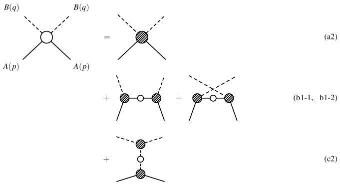
Figure 4: Ingredients of $F_{\mathit{AB}}(\nu)$ in the $A$-$B$ system. The labels represent the correspondence with the self-energy diagrams in Fig. 1.

We then carry out the $q_{\perp}$ integration in Eq. (15) by using the integral formula

$$\int_{-\infty}^{\infty}\frac{d^{2}q_{\perp}}{(2\pi)^{2}}\frac{e^{-L\sqrt{q_{\perp}^{2}+\rho^{2}}}}{2\sqrt{q_{\perp}^{2}+\rho^{2}}}=\frac{1}{4\pi L}e^{-L\rho}\;,$$ (18)

where the integral region can be extended from $\mathbb{B}$ or $\mathbb{B}^{\prime}$ to infinity, because the boundary contributions of $\mathbb{B}$ and $\mathbb{B}^{\prime}$ are already smaller than the order of the error term. Hence, we end up with

$$I_{b1}^{(|\vec{m}|=1)} = \frac{1}{8\pi}\left(\frac{6}{L}\right)\Biggl{[}\frac{\lambda^{2}}{2\nu_{B}}e^{-L\mu}+\int_{-\infty}^{\infty}\!\!\frac{dq_{0}}{2\pi}\;e^{-L\sqrt{q_{0}^{2}+m_{B}^{2}}}\;\{F_{\mathit{AB}}^{(b1-1)}(iq_{0})+F_{\mathit{AB}}^{(b1-2)}(iq_{0})\}\Biggr{]}\!\!$$ (19)

$$+O(e^{-\sqrt{3}L\mu})\;.$$

Other self-energy diagrams in Fig. 1 can be evaluated in a similar way up to $O(e^{-\sqrt{3}L\mu})$, yielding the corresponding 1PI part of the forward scattering amplitude. Note that the contributions from the self-energy diagrams (a1) and (c1) are already smaller than $O(e^{-\sqrt{3}L\mu})$ for $\alpha\in(0,\alpha_{\rm max}]$. By combining all contributions we can discriminate the $|\vec{m}|=1$ contribution up to $O(e^{-\sqrt{3}L\mu})$.

The $|\vec{m}|=\sqrt{2}$ contribution is given by the integral

$$I_{b1}^{(|\vec{m}|=\sqrt{2})} = 12\int\frac{d^{4}q}{(2\pi)^{4}}e^{iL(q_{1}+q_{2})}\Gamma_{\mathit{AAB}}(-p,(1-\eta)p+q;\eta p-q)G_{A}((1-\eta)p+q)$$ (20)

$$\times G_{B}(\eta p-q)\Gamma_{\mathit{AAB}}(p,-(1-\eta)p-q;-\eta p+q)\biggr{|}_{p=(im_{A},\;\vec{0}\,)}\;.$$

Rotating the $q_{1}$-$q_{2}$ axis by $\pi/4$, we define $\tilde{q}_{1}=(q_{1}+q_{2})/\sqrt{2}$ and $\tilde{q}_{2}=(-q_{1}+q_{2})/\sqrt{2}$. Then, apart from the new exponential factor $e^{i\sqrt{2}L\tilde{q}_{1}}$ and an overall factor 12, the integrand becomes exactly the same as in Eq. (6). Thus the evaluation is straightforward and the result is

$$I_{b1}^{(|\vec{m}|=\sqrt{2})} = \frac{1}{8\pi}\left(\frac{12}{\sqrt{2}L}\right)\Biggl{[}\frac{\lambda^{2}}{2\nu_{B}}e^{-\sqrt{2}L\mu}$$ (21)

$$+\int_{-\infty}^{\infty}\!\!\frac{dq_{0}}{2\pi}\;e^{-\sqrt{2}L\sqrt{q_{0}^{2}+m_{B}^{2}}}\;\{F_{\mathit{AB}}^{(b1-1)}(iq_{0})+F_{\mathit{AB}}^{(b1-2)}(iq_{0})\}\Biggr{]}\!\!$$

$$+O(e^{-\sqrt{6}L\mu})\;,$$

where the error term becomes automatically smaller than the $|\vec{m}|=1$ case. Evaluating other diagrams similarly and combining the result of $|\vec{m}|=1$, we arrive at the mass shift formula in Eq. (3).

Finally, let us examine the influence of the $|\vec{m}|=\sqrt{2}$ contribution by looking at the nucleon mass shift in the realistic $N$-$\pi$ system with $m_{N}=938$ MeV and $m_{\pi}=140$ MeV. As the mass ratio is $\alpha=m_{\pi}/m_{N}=0.149$, Eq. (3) is applicable. Moreover, since the formula is valid to all orders in perturbation theory and is expected to hold nonperturbatively, we may insert the empirical $N$-$\pi$ scattering amplitude into Eq. (3). The subthreshold expansion of the $N$-$\pi$ forward scattering amplitude around $\nu=0$ is parametrized as [13]

$$F_{\mathit{N\pi}}(\nu)=6m_{N}D^{+}(\nu)\;,$$ (22)

where

$$D^{+}(\nu)=\frac{g^{2}}{m_{N}}\frac{\nu_{B}^{2}}{\nu_{B}^{2}-\nu^{2}}+d_{00}^{+}\;m_{\pi}^{-1}+d_{10}^{+}\;m_{\pi}^{-3}\nu^{2}+d_{20}^{+}\;m_{\pi}^{-5}\nu^{4}+O(\nu^{6})\;.$$ (23)

The isospin sum is taken in Eq. (22), neglecting the effect of isospin symmetry breaking. The coupling constant is $g^{2}/4\pi=14.3$. The first term in Eq. (23) is identified with the pseudovector nucleon Born term with $\nu_{B}=m_{\pi}^{2}/2m_{N}\approx 0.07m_{\pi}$. The effective coupling is then easily computed by using Eq. (5) as $\lambda^{2}=-12g^{2}\nu_{B}^{2}$. The coefficients of the other terms are given by $d_{00}^{+}=-1.46(10)$, $d_{10}^{+}=1.12(2)$ and $d_{20}^{+}=0.200(5)$ [13]. Hereafter we only take into account the mean of these values.

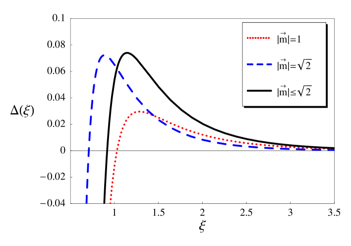
Figure 5: The nucleon mass shift as a function of $\xi=Lm_{\pi}$.

In Fig. 5, we plot $\Delta(\xi=Lm_{\pi})\equiv\Delta m_{N}/m_{N}$ for the $|\vec{m}|=1$ and $|\vec{m}|=\sqrt{2}$ contributions (dotted and dashed lines, respectively) and the sum of these contributions as $|\vec{m}|\leq\sqrt{2}$ (solid line), where $\xi=1$ corresponds to $L=1.4$ fm. It reveals that the $|\vec{m}|=\sqrt{2}$ contribution is quite large for the plotted region of $\xi$. For instance at $\xi=2$ the mass shift is expected to occur more than 1.2 ($|\vec{m}|=1$) + 0.8 ($|\vec{m}|=\sqrt{2}$) = 2.0 % ($\gtrsim$ 20 MeV). If one estimates the $|\vec{m}|=\sqrt{3}$ contribution itself at $\xi=2$,  this merely contributes the mass shift by 0.2 %. This is due to the smaller geometrical factor (e.g. $6$ for $|\vec{m}|=1$, $12/\sqrt{2}\approx 8.49$ for $|\vec{m}|=\sqrt{2}$, and $8/\sqrt{3}\approx 4.62$ for $|\vec{m}|=\sqrt{3}$) as well as the larger exponential decay factor. In this sense the nucleon mass shift formula is significantly modified by discriminating the NLO contribution. Note that the negative mass shift for $\xi\lesssim 1$ is due to the contribution from the term involving the $N$-$\pi$ forward scattering amplitude (ingredients of the $|\vec{m}|=1$ curve can be found in Ref. [10]).

To summarize, we have investigated the finite size mass shift formula for the two stable particle system in a periodic $L^{3}$ box. We have found that it is possible for the mass ratio $\alpha\in(0,\alpha_{\rm max}]$ with $\alpha_{\rm max}\approx 0.418$ to discriminate the NLO contribution with maintaining its model independent structure and validity to all orders in perturbation theory. The final expression is then written as in Eq. (3). Along the way we have also realized that it is impossible to discriminate the NNLO contribution along the line discussed above once the error term is set by $\gamma=2$. In fact, in order to discriminate more higher order contributions, one should go back to the definition of the mass shift in Eq. (1).

We are grateful to the members of lattice forum in DESY theory group in Hamburg, in particular, H. Wittig and I. Montvay for valuable discussions and comments. We appreciate fruitful comments from P. Weisz. Y.K. thanks T.R. Hemmert for useful discussions at the meeting of the DFG Forschergruppe ‘Lattice Hadron Phenomenology’ at DESY-Zeuthen in February.

References

[1]
B. Orth, T. Lippert, and K. Schilling,
Nucl. Phys. B (Proc. Suppl.) 129-130
(2004) 173, hep-lat/0309085.
[2]
G. Colangelo and S. Dürr,
Eur. Phys. J. C33 (2004) 543, hep-lat/0311023.
[3]
QCDSF-UKQCD Collaboration, A. Ali Khan et al.,
Nucl. Phys. B689 (2004) 175, hep-lat/0312030.
[4]
S. R. Beane,
Phys. Rev. D70 (2004) 034507, hep-lat/0403015.
[5]
S. R. Beane,
Nucl. Phys. B695 (2004) 192, hep-lat/0403030.
[6]
W. Detmold and M. J. Savage,
Phys. Lett. B599 (2004) 32, hep-lat/0407008.
[7]
B. Orth, T. Lippert, and K. Schilling,
Finite-size effects in lattice QCD
with dynamical Wilson fermions,
hep-lat/0503016.
[8]
G. Colangelo, S. Dürr, and C. Haefeli,
Finite volume effects for meson masses and decay constants,
hep-lat/0503014.
[9]
G. Colangelo,
Nucl. Phys. B (Proc. Suppl.) 140 (2005) 120,
hep-lat/0409111.
[10]
Y. Koma and M. Koma,
Nucl. Phys. B713 (2005) 575, hep-lat/0406034;
Nucl. Phys. B (Proc. Suppl.) 140 (2005) 329, hep-lat/0409002.
[11]
M. Lüscher,
On a relation between finite size effects
and elastic scattering processes,
Lecture given at Cargese Summer Inst., Cargese,
France, Sep 1-15, 1983, DESY 83-116.
[12]
M. Lüscher,
Commun. Math. Phys. 104, 177 (1986).
[13]
G. Höhler, in: H. Schopper (Ed.), Landolt-Börnstein,
vol. I/9b2, Springer, Berlin, 1983, p. 275, Table 2.4.7.1.