QCD at non-zero temperature and density from the Lattice

Abstract

The study of systems as diverse as the cores of neutron stars and heavy-ion collision experiments requires the understanding of the phase structure of QCD at non-zero temperature, $T$, and chemical potential, $\mu_{q}$. We review some of the difficulties of performing lattice simulations of QCD with $\mu_{q}\neq 0$, and outline the re-weighting method used to overcome this problem. This method is used to determine the critical endpoint of QCD in the $(\mu_{q},T)$ plane. We study the pressure and quark number susceptibility at small $\mu_{q}$.

1 Introduction

The QCD phase diagram is a rich source of interesting phenomena which is key to understanding a wide variety of physical systems, e.g. the early universe, the cores of neutron stars and heavy-ion collisions experiments. Figure 1 illustrates the QCD phase diagram in the chemical potential ($\mu_{q}$) temperature ($T$) plane. It depicts a very rich structure including familiar phases such as nuclear matter, together with very unfamiliar ones such as the colour superconducting phase. See e.g. [1] for further information.

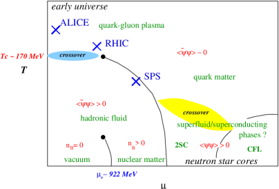
Figure 1: The QCD phase diagram in the temperature-chemical potential plane. First order phase transitions are shown as solid lines, and second order transitions by filled circles. Crosses depict heavy-ion collision experiments. The region of interest in this work is the crossover transition at $T_{c}\approx 170$ MeV.

Lattice simulations of QCD with non-zero chemical potential have recently provided important qualitative and quantitative information on the QCD phase diagram in the $(T,\mu_{q})$ plane [2]. This work will concentrate on studies at finite $T$ and small $\mu_{q}$ which are directly applicable to heavy-ion collision experiments. These are shown as crosses in fig 1 labelled by the name of the relevant experiment.

We begin this paper by outlining the difficulties of simulating QCD with non-zero $\mu_{q}$, and then define the reweighting method which is the basis for much of this work. The method is then used to determine the crossover transition near $\mu=0$ between the confining and deconfining phase (which is depicted as a filled circle in fig 1 near the RHIC point). We also use this method to determine the pressure and quark number susceptibility for QCD. Full details of this work appear in [3] & [4].

2 The Sign Problem

In lattice simulations of QCD at $\mu_{q}=0$, the quark matrix, ${\cal M}(\mu_{q}=0)=D\!\!\!\!/+m$, has the property

$${\cal M}(\mu_{q}=0)=\gamma_{5}{\cal M}^{\dagger}(\mu_{q}=0)\gamma_{5}$$ (1)

which means that the Boltzmann weight is real, and can be interpreted as a probability measure. However, when a non-zero chemical potential is introduced, the quark matrix becomes (schematically) ${\cal M}(\mu_{q})=D\!\!\!\!/+m+\mu_{q}\gamma_{0}$. It therefore no longer has the hermiticity property, and the corresponding Boltzmann weight is complex (the so-called Sign Problem), removing the probabilistic interpretation. This means that the traditional Monte Carlo approach of estimating the path integral is a non-starter.

A number of ways have been promoted to overcome this problem. These fall into two methods. The first is to study models of QCD which, due to their simpler mathematical formulation, do not suffer from the sign problem for $\mu_{q}\neq 0$. Such models include the NJL model and 2-colour QCD. (See [5] for more details.)

The second approach effectively studies QCD at $\mu_{q}=0+\epsilon$ by using either a reweighting technique [6, 7, 8, 3, 9] or an analytical continuation approach [10, 11]. The latter approach simulates with an imaginary $\mu_{q}$ and analytically continues back to the real $\mu_{q}-$axis. The reweighting technique calculates the expectation value of some operator, $\left<{\cal O}\right>$, by factoring off the $\mu_{q}\neq 0$ part of the Boltzmann weight and appending it to the observable ${\cal O}$. Using this approach ensembles generated at $\mu_{q}=0$ can be used. Expressing this idea mathematically we have,

$$\left<{\cal O}\right>_{(\beta,m,\mu)}\!\!\!\!\!\!\!\!\!\!\!\!\!\!\!\!\!\!\!\!\!\!\!\!\!\!\!\!\!\!\!\!\!\!$$ (2)

$$= \frac{1}{{\cal Z}(\beta,m,\mu)}\int{\cal D}U\;{\cal O}\;det{\cal M}(m,\mu)\;e^{-S_{g}(\beta)}$$

$$= \frac{\left<{\cal O}\frac{det{\cal M}(m,\mu)e^{-S_{g}(\beta)}}{det{\cal M}(m_{0},\mu_{0})e^{-S_{g}(\beta_{0})}}\right>_{(\beta_{0},m_{0},\mu_{0})}}{\left<\frac{det{\cal M}(m,\mu)e^{-S_{g}(\beta)}}{det{\cal M}(m_{0},\mu_{0})e^{-S_{g}(\beta_{0})}}\right>_{(\beta_{0},m_{0},\mu_{0})}}$$

$$= \frac{\left<{\cal O}e^{\ln\left(\frac{det{\cal M}(m,\mu)}{det{\cal M}(m_{0},\mu_{0})}\right)-S_{g}(\beta)+S_{g}(\beta_{0})}\right>_{(\beta_{0},m_{0},\mu_{0})}}{\left<e^{\ln\left(\frac{det{\cal M}(m,\mu)}{det{\cal M}(m_{0},\mu_{0})}\right)-S_{g}(\beta)+S_{g}(\beta_{0})}\right>_{(\beta_{0},m_{0},\mu_{0})}}$$

$$= \frac{\left<{\cal O}e^{-W}\right>_{(\beta_{0},m_{0},\mu_{0})}}{\left<e^{-W}\right>_{(\beta_{0},m_{0},\mu_{0})}}.$$

In these equations, $S_{g}$ is the gauge action, $U$ denotes the gauge degrees of freedom, $\beta=6/g^{2}$, where $g$ is the gauge coupling, and we have introduced the dimensionless lattice chemical potential, $\mu=\mu_{q}a$. By setting $\mu_{0}$ to zero, eq(2) enables the calculation of quantities at $\mu\neq 0$ using ensembles generated at $\mu_{0}=0$.

The results presented in this work are derived from the reweighting approach as well as a Taylor expansion of $\left<{\cal O}\right>$ about $\mu_{q}=0$.

3 Lattice details

Our simulations were performed on a $N_{s}^{3}\times N_{t}=16^{3}\times 4$ lattice with two (degenerate) quark flavours (see [3] [4] for full details). We used two different quark masses, $ma=$ 0.1 and 0.2 corresponding to pseudoscalar-vector meson mass ratios of $M_{PS}/M_{V}\approx$ 0.70 and 0.85 respectively [12]. A Symanzik improved gauge action together with the p4 improved quark action [13] was used to reduce lattice discretisation artefacts.

A range of $\beta$ values was simulated, each corresponding to a different temperature via the usual relationship, $T=1/(a(\beta)N_{t})$, where $N_{t}$ is the number of lattice sites in the temporal direction. ${\cal O}(1,000,000)$ trajectories were generated in this project using the APEmille computers in Bielefeld and Swansea.

4 Reweighting preliminaries

As an illustration of the reweighting method we show the susceptibility of the chiral condensate, $\chi_{\overline{\psi}\psi}$ as a function of $\beta$ in fig 2 for a quark mass of $ma=0.1$. Note that to produce this plot, a reweighting has been performed both in $\beta$ and $\mu$ (i.e. the simulations were only performed a relatively coarse values of $\beta$ compared to those shown in fig 2).

Figure 2: The chiral susceptibility, $\chi_{\overline{\psi}\psi}(\beta)$ at $ma=0.1$ for various $\mu$.

As can be seen, there is a clear peak in the susceptibility, which occurs at the crossover transition. This means that the expectation value of $\overline{\psi}\psi$ fluctuates strongly at this $\beta$ value corresponding to a temperature $T=1/(a(\beta)N_{t})$. By mapping out the position of this transition as a function of $\beta$ and $\mu$, the phase diagram, fig 3, can be obtained [3].

Note that figs 2 and 3 were obtained by Taylor expanding the susceptibilities to ${\cal O}(\mu^{2})$. The phase diagram, fig 3 is therefore correct to this order in $\mu$ [3].

Figure 3: The phase diagram obtained from our reweighting technique. The errors shown are statistical. The diamond is the endpoint of the first order phase transition obtained by Fodor and Katz [7].

5 Pressure

The pressure is related to the grand partition function, ${\cal Z}(T,V,\mu_{q})$ by

$$\frac{p}{T^{4}}=\frac{1}{VT^{3}}\ln{\cal Z}.$$ (3)

We can now Taylor expand both sides of this equation in the dimensionless ratio $\mu_{q}/T$. Since we can only utilize Monte Carlo methods at $\mu_{q}\equiv 0$, we perform this expansion about this point obtaining

$$\Delta\left(\frac{p}{T^{4}}(\mu_{q})\right) \equiv \frac{p}{T^{4}}\biggr{|}_{T,\mu_{q}}-\frac{p}{T^{4}}\biggr{|}_{T,0}$$ (4)

$$\!\!\!\!\!\!\!\!\!\!\!\!\!\!\!\!\!\!\!\!\!\!\!\!\!\!\!\!\!\!\!\!\!\!\!\!\!= \!\!\!\!\!\!\!\!\!\!\!\!\!\!\!\!\!\!\!\!\frac{1}{2!}\frac{\mu_{q}^{2}}{T^{2}}\frac{\partial^{2}(p/T^{4})}{\partial(\mu_{q}/T)^{2}}+\frac{1}{4!}\frac{\mu_{q}^{4}}{T^{4}}\frac{\partial^{4}(p/T^{4})}{\partial(\mu_{q}/T)^{4}}+\ldots$$

$$\!\!\!\!\!\!\!\!\!\!\!\!\!\!\!\!\!\!\!\!\!\!\!\!\!\!\!\!\!\!\!\!\!\!\!\!\!\equiv \!\!\!\!\!\!\!\!\!\!\!\!\!\!\!\!\!\!\!\!\sum_{n=2,4,\ldots}^{\infty}c_{n}(T)\;\;\left(\frac{\mu_{q}}{T}\right)^{n},$$

where all derivatives are taken at $\mu_{q}=0$. Only even powers occur in eq(4) because odd derivatives of the free energy with respect to $\mu_{q}$ vanish [3]. Using eq(3), the derivatives in eq(4) can be expressed as expectation values (over a $\mu_{q}=0$ ensemble).

In figs 4 and 5 the first two coefficients of $p$, $c_{2,4}$, are plotted as a function of temperature. For comparison, the Stefan-Boltzmann (SB) values are plotted. These are valid in the limit of infinite temperature, where the system becomes asymptotically free. The continuum SB expression for massless quarks is

$$\frac{p_{SB}}{T^{4}}(\mu_{q})=\frac{7N_{f}\pi^{2}}{60}+\frac{N_{f}}{2}\left(\frac{\mu_{q}}{T}\right)^{2}+\frac{N_{f}}{4\pi^{2}}\left(\frac{\mu_{q}}{T}\right)^{4},$$

so the coefficients $c_{2,4}$ can be simply read-off. Also shown in figs 4 and 5 are SB values corresponding to a free field lattice calculation at $N_{t}=4$ (i.e. corresponding to the temporal extent of our lattice, see sec. 3). The details of this calculation can be found in [4]. As can be seen from figs 4 and 5, both $c_{2}$ and $c_{4}$ vary sharply in the critical region, $T\approx T_{0}$.

Figure 4: The quadratic coefficient of the Taylor expansion of the pressure, $c_{2}$, as a function of temperature. (See eq(4).)

Figure 5: The quartic coefficient of the Taylor expansion of the pressure, $c_{4}$, as a function of temperature. (See eq(4).)

Using the coefficients $c_{2,4}$, we plot the pressure difference, $\Delta(p/T^{4})$ as a function of temperature for various $\mu_{q}/T$ in fig 6. Again we observe an abrupt change in the pressure as the critical region is crossed. It is interesting to note that the pressure at finite density is very similar to its $\mu_{q}=0$ value. For instance, at the RHIC point ($\mu_{q}/T\approx 0.1$) the pressure is only 1% more than its zero density value.

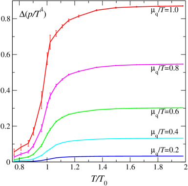
Figure 6: The dimensionless pressure difference $\Delta(p/T^{4})$ as a function of temperature for various $\mu_{q}/T$ values.

6 Susceptibility

We turn our discussion to the quark number density, $n_{q}$, and its susceptibility, $\chi_{q}$, defined as,

$$\frac{n_{q}}{T^{3}} = \frac{\partial(p/T^{4})}{\partial(\mu_{q}/T)}$$

$$\frac{\chi_{q}}{T^{2}} = \frac{\partial^{2}(p/T^{4})}{\partial(\mu_{q}/T)^{2}}.$$

The ingredients required to calculate the susceptibility have already been determined in the Taylor expansion of the pressure (see eqs(3 & 4)). Figure 7 plots $\chi_{q}/T^{2}$ as a function of temperature for various $\mu_{q}/T$ values. As can be seen, a peak in $\chi_{q}$ develops at $T\approx T_{0}$ which grows with $\mu_{q}$. This is a signal of a critical endpoint in the $(\mu_{q},T)$ plane where the fluctuations in the number operator $\overline{\psi}\gamma_{0}\psi$ grow. Also note that the peak occurs at $T=T_{0}$, implying that the chiral symmetry restoration transition observed in fig 2 and the deconfinement transition of fig 7 coincide [1].

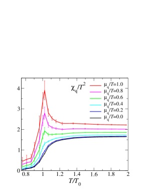
Figure 7: The quark number susceptibility, $\chi_{q}$, as a function of temperature, for various $\mu_{q}/T$ values.

7 Conclusions

We have presented some results of studies of QCD at non-zero temperature and small chemical potential [3, 4]. In particular we have summarised the difficulties in using conventional Monte Carlo techniques to perform lattice simulations of QCD at non-zero $\mu$. We outlined the reweighting technique which has recently been very successful in obtaining numerical results at $\mu\neq 0$, despite this difficulty [7, 3]. This method was used to determine the position of the crossover transition between the confined and de-confined phases. Finally, results for the pressure and susceptibility were produced, based on a Taylor expansion in $\mu_{q}/T$.

References

- [1] H. Satz, Nucl.Phys. A681 (2001) 3.
- [2] S.D. Katz, Plenary Talk at Lattice 2003, hep-lat/0310051.
- [3] C.R. Allton, S. Ejiri, S.J. Hands, O. Kaczmarek, F. Karsch, E. Laermann, Ch. Schmidt and L. Scorzato, Phys. Rev. D66 (2002) 074507.
- [4] C.R. Allton, S. Ejiri, S.J. Hands, O. Kaczmarek, F. Karsch, E. Laermann and C. Schmidt, Phys. Rev. D68 (2003) 014507.
- [5] S.J. Hands, Nucl. Phys. B (Proc. Suppl.) 106 (2002) 142.
- [6] S. Gottlieb, W. Liu, D. Toussaint, R.L. Renken and R.L. Sugar, Phys. Rev. D38 (1988) 2888.
- [7] Z. Fodor and S.D. Katz, JHEP 0203 (2002) 014; Phys. Lett. B534 (2002) 87.
- [8] S. Choe et al. (QCDTARO Collaboration), Phys.Rev. D65 (2002) 054501.
- [9] R.V. Gavai and S. Gupta, Phys.Rev. D68 (2003) 034506.
- [10] P. De Forcrand and O. Philipsen, Nucl. Phys. B642 (2002) 290.
- [11] M. D’Elia and M.-P. Lombardo, Phys.Rev. D67 (2003) 014505.
- [12] F. Karsch, E. Laermann and A. Peikert, Phys. Lett. B478 (2000) 447; Nucl. Phys. B605 (2001) 579.
- [13] U.M. Heller, F. Karsch and B. Sturm, Phys. Rev. D60 (1999) 114502.