A Euclidean Lattice Construction of Supersymmetric Yang-Mills Theories with Sixteen Supercharges

Abstract:

We formulate supersymmetric Euclidean spacetime $A_{d}^{*}$ lattices whose classical continuum limits are $U(N)$ supersymmetric Yang-Mills theories with sixteen supercharges in $d=1,2,3$ and $4$ dimensions. This family includes the especially interesting ${\cal N}=4$ supersymmetry in four dimensions, as well as a Euclidean path integral formulation of Matrix Theory on a one dimensional lattice.

1 Introduction

Sixteen is the maximal number of supercharges that can be accommodated in a theory with particle multiplets of spin $s\leq 1$. Such theories are extremely constrained and much is known or surmised about them. The ${\cal Q}=16$ $SU(N)$ gauge theory in $d=4$ dimensions, known as ${\cal N}=4$ supersymmetry, is believed to be finite and superconformal, possessing monopole and dyon excitations [1, 2], as well as a discrete $SL(2,Z)$ symmetry generalizing electric-magnetic duality [3, 4] which exchanges weak and strong coupling. In the large $N$ limit, the theory is conjectured to be equivalent to supergravity in $AdS_{5}$ space [5, 6, 7]. The $d=3$ theory with ${\cal Q}=16$ supercharges is expected to have a nontrivial infrared fixed point [8], while in $d=1$ and $d=0$ dimensions, the respective quantum mechanical and matrix theories are conjectured to be related in the large-$N$ limit to $M$-theory[9, 10]. Despite the intense interest in these theories, and the obvious need for a nonperturbative definition, none existed until their construction on a spatial lattice in ref. [11]. In this paper we continue the program of refs. [12, 13] and show how the ${\cal Q}=16$ supercharge theories may be constructed on Euclidean spacetime lattices; as we shall show, the $A_{d}^{*}$ structure of the lattices we construct have a particularly elegant structure.

The challenge confronting attempts to put these and other supersymmetric Yang-Mills (SYM) theories on the lattice has been how to maintain enough supersymmetry in the absence of continuous translations in order to forbid the numerous relevant operators which violate the symmetries of the desired continuum theory. Obvious and egregious examples of such unwanted operators are mass terms for the scalar partners of the gauge bosons; only some sort of residual supersymmetry can forbid such operators. However, early attempts to construct supersymmetric lattices failed to yield Lorentz invariant continuum field theories [17]. Recently two approaches have been developed for constructing lattices respecting exact supersymmetries, which yield Lorentz invariant supersymmetric theories in the continuum with either no or little fine tuning. The approach pioneered by Catterall and collaborators and followed up by Sugino starts with nilpotent charges which form a subset of the supercharges of the target theory[18, 19, 20, 21, 22, 23, 24, 25]. The approach followed here creates the lattice theories by performing an orbifold projection on supersymmetric matrix models obtained by dimensionally reducing SYM theories in various dimensions[11, 12, 13]; for a review see [14]. The projection creates a lattice action while preserving some of the supersymmetries of the matrix model. The theories have a degenerate manifold of ground states in the infinite volume limit (the moduli space), where the distance from the origin in moduli space is identified as the inverse lattice spacing of the theory. The continuum limit is thus defined as a trajectory out to infinity in the moduli space, and the result is a SYM field theory. Again, the exact supersymmetries of the lattice guarantee that the continuum limit can be achieved with little or no fine tuning. This method for constructing supersymmetric lattice theories has its origins in orbifold projection methods of string theory [26] and deconstruction [27, 28, 29]. In the next section we address generalities of the construction, and then we discuss each case in turn, from dimension $d=4$ down to $d=1$.

2 The mother theory and the orbifold projection

2.1 The mother theory

Our starting point is the ${\cal Q}=16$ mother theory, which is the dimensional reduction of N=1 SYM with gauge group ${\cal G}$ from ten Euclidean dimensions down to zero dimensions. The mother theory is a theory of matrices — ten bosonic and sixteen Grassmann — and inherits the sixteen supersymmetries as well as the ${\cal G}\times SO(10)$ symmetry of its ten-dimensional precursor. Each of the bosons and fermions transform as an adjoint under ${\cal G}$, while under the $SO(10)$ symmetry they transform as the $\boldsymbol{10}$ and $\boldsymbol{16}$ representations respectively. We choose a Hermitean chiral basis for the ten, 32-dimensional gamma matrices $\Gamma_{\alpha}$ of $SO(10)$, and the chirality matrix $\Gamma_{11}$ satisfying

$$\{\Gamma_{\alpha},\Gamma_{\beta}\}=2\delta_{\alpha\beta}\ ,\qquad\Gamma_{\alpha}=\Gamma_{\alpha}^{\dagger}\ ,\qquad\Gamma_{11}=-i\prod_{\alpha=1}^{10}\Gamma_{\alpha}\ .$$ (1)

The generators of $SO(10)$ transformations are given by

$$M_{\alpha\beta}=\frac{1}{4i}\left[\Gamma_{\alpha},\Gamma_{\beta}\right]\ ,$$ (2)

and the charge conjugation matrix $C$ satisfies

$$C^{-1}\Gamma_{\alpha}C=-\Gamma_{\alpha}^{T}\ ,\qquad C^{\dagger}=C^{-1}=C\ .$$ (3)

For greater ease in comparing lattice and continuum theories, we will choose the convention

$$\Gamma_{m}^{T}=\begin{cases}-\Gamma_{m}&m=1,\ldots,5\cr+\Gamma_{m}&m=6,\ldots,10\end{cases}$$ (4)

allowing us to define the charge conjugation matrix as

$$C=\prod_{m=1}^{5}\,\Gamma_{m}\ .$$ (5)

For an explicit $\Gamma$ matrix basis worked out in detail, see Appendix A.

We define a left-handed Grassmann spinor $\omega=+\Gamma_{11}\omega$ which is written as a 32-component Dirac spinor, but which only has 16 independent components and transforms as the irreducible ${\bf 16}$ representation of $SO(10)$. We also introduce a real bosonic variable $v_{\alpha}$ transforming as the ${\bf 10}$ representation of $SO(10)$. Then the action of the mother theory may be written as

$$S=\frac{1}{g^{2}}\left(\frac{1}{4}\operatorname{Tr\,}v_{\alpha\beta}v_{\alpha\beta}+\frac{i}{2}\operatorname{Tr\,}\omega^{T}\,C\,\Gamma_{\alpha}\,[v_{\alpha},\omega]\ \right)$$ (6)

where $v_{\alpha\beta}=i[v_{\alpha},v_{\beta}]$. In this expression $\omega=\omega^{a}T_{a}$ and $v_{\alpha}=v_{\alpha}^{a}T_{a}$ are matrices, where $T_{a}$ are the hermitean generators of ${\cal G}$ in the defining representation of ${\cal G}$, normalized so that

$$\operatorname{Tr\,}T_{a}T_{b}=\delta_{ab}\ .$$ (7)

The global $G_{R}=SO(10)$ symmetry of the above action is just the ten dimensional Lorentz symmetry transmuted to a global symmetry of the zero dimensional mother theory. Explicitly, the fermionic and bosonic fields transform under $SO(10)$ as

$$\omega\to\Omega\omega,\qquad\hbox{\kern 2.5pt\raise 0.77496pt\hbox{$/$}\kern-6.00006pt$v$}\to\Omega\,\hbox{\kern 2.5pt\raise 0.77496pt\hbox{$/$}\kern-6.00006pt$v$}\,\Omega^{-1}\ ,\qquad\hbox{\kern 2.5pt\raise 0.77496pt\hbox{$/$}\kern-6.00006pt$v$}\equiv\Gamma_{\alpha}v_{\alpha}\ ,\qquad\Omega\in SO(10)\ .$$ (8)

One can also show that the action eq. (6) is invariant under the supersymmetry transformation,

$$\delta v_{\alpha}=-\kappa^{T}C\Gamma_{\alpha}\omega\ ,\qquad\delta\omega=iv_{\alpha\beta}M_{\alpha\beta}\kappa\ ,$$ (9)

where $\kappa$ is a chiral Grassmann spinor satisfying $\Gamma_{11}\kappa=+\kappa$ with 16 independent components parameterizing the ${\cal Q}=16$ supersymmetry of the mother theory. Note that the supersymmetry transformations do not commute with $SO(10)$, and that $\kappa$ (and hence the supercharges) transform as a $\boldsymbol{16}$.

2.2 Specifying the orbifold projection

The procedure of creating lattices by using the orbifold projection technique has been explained in detail in [12, 13], and we summarize it briefly here. To construct the a $d$-dimensional lattice with $N$ sites in each direction for a target theory possessing a $U(k)$ gauge symmetry and in the continuum, we choose the group ${\cal G}$ of the mother theory to be ${\cal G}=U(kN^{d})$. Each of the variables of the mother theory are therefore $kN^{d}$-dimension matrices. We then project out all variables in the mother theory which are charged under a certain $Z_{N}^{d}$ subgroup of the $U(kN^{d})\times SO(10)$ symmetry of the mother theory, and the action written in terms of the surviving variables has a natural lattice interpretation. The structure and symmetries of the lattice depend on the embedding of the discrete $Z_{N}^{d}$ subgroup.

The embedding of the discrete $Z_{N}^{d}$ subgroup within $U(kN^{d})$ is given by the natural decomposition $U(k)^{Nd}\ltimes Z_{N}^{d}$. It is convenient to consider each one of the bosonic or fermionic matrices of the mother theory, which we will refer to generically as $\Phi$, to be a matrix consisting of $N^{2d}$ independent $k\times k$ blocks. These blocks can be written as $\Phi_{{\bf m},{\bf n}}$, where ${\bf m}$ and ${\bf n}$ are two independent $d$-dimensional vectors with integer components, each of which run from $1$ to $N$. This action of the mother theory eq. (6) can be considered as an extremely nonlocal lattice action in $d$-dimensions, where each site is labeled by a $d$-dimensional integer vector ${\bf m}$, and each nonzero block $\Phi_{{\bf m},{\bf n}}$ is a a $k\times k$ matrix valued lattice variable living on the link between sites ${\bf m}$ and ${\bf n}$. In the case where ${\bf m}={\bf n}$, the diagonal $\Phi_{{\bf m},{\bf m}}$ block is a variable sitting at the site ${\bf m}$.

The orbifold projection sets most of these lattice blocks to zero. In particular, each $\Phi$ variable is assigned a $Z_{N}^{d}$ charge ${\bf r}$ according to its weight vector in $SO(10)$, where ${\bf r}$ is a $d$-component vector with integer coefficients running from $1$ to $N$. The exact relation between ${\bf r}$ and the $SO(10)$ weights will be discussed further below. The orbifold projection then sets to zero all blocks $\Phi_{{\bf m},{\bf n}}$ not satisfying ${\bf n}={\bf m}+{\bf r}$. If all components of the ${\bf r}$ vectors equal zero or $\pm 1$, then the action eq. (6) written in terms of the projected variables will look like a very local lattice action.

The projection breaks the original ${\cal G}=U(kN^{d})$ symmetry of the mother theory down to an independent $U(k)$ symmetry associated with each lattice site, which constitutes the lattice version of a $U(k)$ gauge symmetry. Each site variable transforms as an adjoint under the local $U(k)$ symmetry, while each link variable transforms as a bifundamental $(\raisebox{-0.5pt}{\hbox{\rule{0.4pt}{6.5pt}\hskip-0.4pt\rule{6.5pt}{0.4pt}\hskip-6.5pt\rule[6.5pt]{6.5pt}{0.4pt}}\rule[6.5pt]{0.4pt}{0.4pt}\hskip-0.4pt\rule{0.4pt}{6.5pt}},\kern 0.6pt\overline{\kern-0.6pt\raisebox{-0.5pt}{\hbox{\rule{0.4pt}{6.5pt}\hskip-0.4pt\rule{6.5pt}{0.4pt}\hskip-6.5pt\rule[6.5pt]{6.5pt}{0.4pt}}\rule[6.5pt]{0.4pt}{0.4pt}\hskip-0.4pt\rule{0.4pt}{6.5pt}}\kern-0.6pt}\kern 0.6pt)$ or its conjugate under the $U(k)\times U(k)$ symmetries associated with the endpoints of the links.

The orbifold projection breaks some or all of the supersymmetries of the mother theory. That is because the supercharges are transform as a spinor under $SO(10)$, but are ${\cal G}$-invariant. Thus only supercharges with ${\bf r}=0$ survive the orbifold projection.

It remains to specify how the ${\bf r}$ charges are related to the $SO(10)$ symmetry. Our choice of how to embed the $Z_{N}^{d}$ symmetry into $SO(10)$ is guided by three principles:

1. Since we will eventually take $N\to\infty$, the embedding must take the form $Z_{N}^{d}\in U(1)^{d}\in SO(10)$;

2. Supersymmetry generators $Q$ are ${\cal G}$-invariant and transform as a $\boldsymbol{16}$ of $SO(10)$. Therefore, in order to break as few supersymmetries as possible, for any lattice dimension $d$ we will want to maximize the number of elements in the spinor of $SO(10)$ which are singlets under the $Z_{N}^{d}$ symmetry (e.g. which have ${\bf r}=0$);

3. Lattice variables associated with the surviving $({\bf m},{\bf n})=({\bf m},{\bf m}+{\bf r})$ block of a mother theory variable $\Phi$ resides on the link between sites ${\bf m}$ and ${\bf m}+{\bf r}$. Therefore, in order to keep the lattice action as local as possible, we want the components of ${\bf r}$ to all be $0$ or $\pm 1$, to avoid having link variables connecting distant sites.

The first point implies that the $Z_{N}^{d}$ orbifold group should be embedded within the $U(1)^{5}$ Cartan subgroup of $SO(10)$. It immediately follows that the maximum lattice dimension we could construct in this manner is $d=5$. (We will see that requiring that the lattice be supersymmetric will actually constrain the maximum dimension to be $d=4$). We can take the five generators $q_{m}$ of this $U(1)^{5}$ symmetry to be

$$q_{m}=M_{m,m+5}\ ,\quad m=1,\ldots,5$$ (10)

corresponding to rotations in the $x_{m}-x_{m+5}$ plane in a ten dimensional space.

The five complex bosonic fields

$$z_{m}=i(v_{m}-iv_{m+5})/\sqrt{2}\ ,\qquad\kern 0.6pt\overline{\kern-0.6ptz\kern-0.6pt}\kern 0.6pt_{m}=-i(v_{m}+iv_{m+5})/\sqrt{2}$$ (11)

are eigenstates of the $U(1)^{5}$ symmetry generated by the $q_{m}$, where $z_{m}$ has charge $q_{n}=\delta_{mn}$, and $\kern 0.6pt\overline{\kern-0.6ptz\kern-0.6pt}\kern 0.6pt_{m}$ has charge $q_{n}=-\delta_{mn}$.

The charges of the fermions are determined by defining the anticommuting raising and lowering operators

$$\hat{A}^{m}={\textstyle{\frac{1}{2}}}\left(\Gamma_{m}-i\Gamma_{m+5}\right),\qquad\hat{A}_{m}^{\dagger}={\textstyle{\frac{1}{2}}}\left(\Gamma_{m}+i\Gamma_{m+5}\right),\qquad m=1,\ldots,5,$$ (12)

which satisfy the relations

$$\{\hat{A}^{m},\hat{A}^{n}\}=\{\hat{A}_{m}^{\dagger},\hat{A}_{n}^{\dagger}\}=0,\qquad\{\hat{A}^{m},\hat{A}_{n}^{\dagger}\}=\delta^{m}_{n},$$ (13)

familiar as the algebra of fermionic ladder operators. The spinor representation is then constructed in a Fock space of five different species of one-component fermion, each of which has occupation number zero or one. The operators forming Cartan subalgebra of $SO(10)$ can be expressed in terms of these fermionic raising and lowering operators as

$$q_{m}=M_{m,m+5}=\left(\hat{A}_{m}^{\dagger}\hat{A}^{m}-{\textstyle{\frac{1}{2}}}\right)\qquad\text{(no sum on $m$).}$$ (14)

The 32-dimensional reducible spinor representation thus consists of the states with $q_{m}$ charges

$$|\pm{\textstyle{\frac{1}{2}}},\pm{\textstyle{\frac{1}{2}}},\pm{\textstyle{\frac{1}{2}}},\pm{\textstyle{\frac{1}{2}}},\pm{\textstyle{\frac{1}{2}}}\rangle$$ (15)

The 16-dimensional irreducible representations are found by projecting out those states with $\Gamma_{11}=\pm 1$. As $\Gamma_{11}=-i\prod_{\alpha=1}^{10}\Gamma_{\alpha}=\prod_{m=1}^{5}(2q_{m})$, the ${\bf 16}$ of $SO(10)$ consists of states with $q_{m}$ charges given by the 32 states in eq. (15), subject to the additional constraint

$$\prod_{m=1}^{5}\,2q_{m}=+1\ .$$ (16)

The $Z_{N}^{d}$ orbifold symmetry is then embedded in $SO(10)$ by defining the ${\bf r}$ charges in terms of the five $q_{m}$. The three guidelines above may be economically satisfied if we define

$$r_{\mu}=q_{\mu}-q_{d+1}\ ,\qquad\mu=1\,\ldots,d\leq 4\ .$$ (17)

With this definition we see that each of the components of ${\bf r}$ only assumes the values $\pm 1$ or $0$ for any of the bosonic or fermionic variables of the mother theory. This fulfills our requirement that the orbifold projection be chosen so that there are only neighbor interactions on the resulting lattice. Furthermore, it follows that $2^{4-d}$ of the sixteen fermions have vanishing ${\bf r}$, which is the maximum possible. With the above definition of ${\bf r}$ we can construct $d$-dimensional local lattices with $2^{4-d}$ unbroken supercharges. We will consider below all the lattices with $d\leq 4$, and will display the ${\bf r}$ charges explicitly in each case.

The $d$ ${\bf r}$ charges generate the Cartan subgroup of an $SU(d+1)$ subgroup of the original $SO(10)$, an observation which proves useful in constructing the lattice theories, as it implies that the position on the lattice assigned to each variable is determined by its $SU(d+1)$ weight. To see this, note that the anticommutation relations eq. (13) imply that the operators

$$\hat{T}_{a}\equiv\hat{A}^{\dagger}_{m}(T_{a})^{m}_{\ n}\hat{A}^{n}\ ,\qquad m,n=1,\ldots,5\ ,$$ (18)

satisfy the commutation relations

$$\left[\hat{T}_{a},\,\hat{T}_{b}\right]=\hat{A}^{\dagger}_{m}\left[T_{a},\,T_{b}\right]^{m}_{\ n}\hat{A}^{n}\ .$$ (19)

The components of ${\bf r}$ defined in eq. (17) may be written as

$$r_{\mu}=\hat{A}^{\dagger}_{m}(R_{\mu})^{m}_{\ n}\hat{A}^{n},\qquad(R_{\mu})^{m}_{\ n}\equiv(\delta^{m}_{\mu}\delta_{n\mu}-\delta^{m}_{5}\delta_{n}^{5})\ ,\qquad\mu=1,\ldots,d.$$ (20)

Since the $R_{\mu}$ matrices are linearly independent, real, diagonal and traceless, it follows that the four ${\bf r}$ charges generate the Cartan subalgebra of an $SU(d+1)$ subgroup of $SO(10)$.

2.3 From orbifold projection to spacetime lattice

As described above, the orbifold projection gives rise to an action which can be conveniently described as a lattice action, assigning variables to links and sites of a $d$-dimensional lattice as determined by their ${\bf r}$ charges. However, at this point the lattice does not resemble a spacetime lattice (for example, the action derived from eq. (6) has only cubic and quartic terms, and nothing resembling a kinetic “hopping term”. Furthermore, there is no intrinsic dimensionful scale in the action, and hence no metric or definition of distance given to our lattice links. All that is defined by the action of the orbifold theory is a connectivity. This can be made precise by recognizing that the ${\bf m}$ and ${\bf n}={\bf m}+{\bf r}$ vectors are not themselves lattice vectors. Instead, the lattice point ${\bf m}$ resides at spacetime point $\vec{x}=\sum_{a}m_{a}\vec{e}_{a}\equiv{\bf m}\cdot\vec{\bf e}$, where the $\vec{e}_{a}$ are a complete set of lattice vectors, to be specified. Similarly, link variables associated with the vector ${\bf r}$ reside on links corresponding to the spacetime vector ${\bf r}\cdot\vec{\bf e}$.

As seen in earlier examples [11, 12, 13, 14], turning the orbifold lattice into a spacetime lattice is accomplished by expanding the orbifold projected action about a certain point in moduli space. The vacuum expectation values of the bosonic link variables at this point in moduli space are interpreted as the inverse lengths of the corresponding links of the spacetime lattice, and the continuum limit is taken by moving out to infinity in moduli space . Expanding about different points in moduli space can leave intact different symmetries, and correspond to different spacetime lattice structures. For example, if we were to choose the point where the $z_{m}$ and $\kern 0.6pt\overline{\kern-0.6ptz\kern-0.6pt}\kern 0.6pt^{m}$ variables were equal and proportional to the identity matrix for those with $r_{a}=\delta_{ai}$ for $i=1,\ldots,d$, with all other bosonic variables vanishing, the resultant $d$-dimensional lattice would be hypercubic, with various diagonal link variables. However, as we will show below, the most symmetric choice corresponds to not to an $A_{d}^{*}$ lattice, rather than a hypercubic one.

We now turn to the explicit construction of the supersymmetric lattices in dimensions $d=1,\ldots,4$. In particular, we write down the orbifold action for dimension $d$, and make explicit the exact supersymmetry retained on the lattice. We then show how the desired target theory is obtained at the classical level as one travels along the $A_{d}^{*}$ trajectory in moduli space, described in the previous section, making explicit the peculiar way in which the lattice variables assemble themselves into the continuum variables of the ${\cal Q}=16$ target theory, which typically form large multiplets of both supersymmetry and a chiral $R$-symmetry. For more information about these target theories, we refer the reader to ref. [8].

3 Construction of the lattice in four dimensions

3.1 The target theory

For $d=4$ the continuum target theory with ${\cal Q}=16$ supercharges is ${\cal N}=4$ SYM theory with a $U(k)$ gauge group. The action for this theory can be simply obtained by dimensional reduction of the simple ${\cal N}=1$ SYM theory in ten dimensions down to four dimensions. The action therefore possesses a global $SO(4)\times SO(6)$ symmetry inherited by dimensional reduction (where the $SO(4)\simeq SU(2)\times SU(2)$ is the Euclidean version of the Lorentz symmetry, and $SO(6)\simeq SU(4)$ is called the $R$-symmetry of the theory). The gauge fields $v_{\alpha}$ of the ten-dimensional theory reduce to four gauge fields $V_{\mu}$ in four dimensions, plus six scalar fields $S_{a}$. The sixteen component gaugino $\tilde{\omega}$ of the ten-dimensional theory reduces to four complex Weyl doublet fermions. The transformations of these fields is

$$\begin{array}[]{c|c}&SO(6)\times SU(2)\times SU(2)\cr\hline\cr V_{\mu}&(1,2,2)\cr S_{a}&(6,1,1)\cr\tilde{\omega}&(4,2,1)\oplus(\kern 0.6pt\overline{\kern-0.6pt4\kern-0.6pt}\kern 0.6pt,1,2)\end{array}$$ (25)

In order to make a direct connection between the lattice and the continuum theory, it is simplest to express the target action in four dimensions in a notation that retains some of the structure inherited from ten dimensions. Therefore we write the action for ${\cal N}=4$ SYM in four dimensions as

$$S_{\text{target}} = \frac{1}{g_{4}^{2}}\,\int d^{4}{\bf R}\,\operatorname{Tr\,}\Bigl{(}\frac{1}{4}V_{\mu\nu}V_{\mu\nu}+\frac{1}{2}(D_{\mu}S_{a})^{2}-\frac{1}{4}\left[S_{a},S_{b}\right]^{2}$$ (27)

$$\qquad\qquad\qquad\qquad+\frac{1}{2}\tilde{\omega}^{T}\,\tilde{C}\,D_{\mu}\,\tilde{\Gamma}_{\mu}\,\tilde{\omega}+\frac{i}{2}\,\tilde{\omega}^{T}\,\tilde{C}\,\tilde{\Gamma}_{4+a}\,[S_{a},\tilde{\omega}]\Bigr{)}$$

Here we have introduced $SO(10)$ gamma matrices $\tilde{\Gamma}_{\alpha}$ and charge conjugation matrix $\tilde{C}$ . The $SO(4)\times SO(6)$ invariance of the above theory is manifest.

3.2 The mother theory in $SU(5)\times U(1)$ multiplets

To create a four dimensional lattice from the ${\cal Q}=16$ mother theory, we orbifold by $Z_{N}^{4}$, where the four $Z_{N}$ transformations are determined by the four-vector ${\bf r}$ charges defined in eq. (17) with $d=4$. As we showed in §2.2, the ${\bf r}$ charges generate the Cartan subgroup of the $SU(5)$ subgroup of the original $SO(10)$ symmetry of the mother theory, and that the assignment of variables of the mother theory onto links and sites of the lattice follows from their $SU(5)$ weights. It is convenient therefore to decompose the variables of the mother theory under the subgroup $SU(5)\times U(1)\in SO(10)$, where the $U(1)$ is generated by

$$Q_{0}\equiv\sum_{m=1}^{5}q_{m}\qquad\text{($U(1)$ generator)}\ ,$$ (28)

where the $q_{m}$ are defined in eq. (10); $Q_{0}$ generates a rotation in all of the $m$, $m+5$ planes of the ten dimensional space simultaneously.

The bosons $v_{\alpha}$ transform as a 10 of $SO(10)$ and decompose under as the $SU(5)\times U(1)$ subgroup as

$$v\sim{\bf 10}\ \longrightarrow\ z\oplus\kern 0.6pt\overline{\kern-0.6ptz\kern-0.6pt}\kern 0.6pt\sim{\bf 5_{1}}\oplus{\bf\kern 0.6pt\overline{\kern-0.6pt5\kern-0.6pt}\kern 0.6pt_{-1}}\ .$$ (29)

It should be evident that the $z_{m}$ and $\kern 0.6pt\overline{\kern-0.6ptz\kern-0.6pt}\kern 0.6pt_{m}$ variables defined in eq. (11) have $U(1)$ charges $Q_{0}=+1$ and $Q_{0}=-1$ respectively, and so it must be that $z_{m}\sim{\bf 5_{1}}$ and $\kern 0.6pt\overline{\kern-0.6ptz\kern-0.6pt}\kern 0.6pt_{m}\sim{\bf\kern 0.6pt\overline{\kern-0.6pt5\kern-0.6pt}\kern 0.6pt_{-1}}$. As for the fermions, the variable $\omega$ of the mother theory, transforming as a 16 of $SO(10)$, decomposes under $SU(5)\times U(1)$ as

$$\omega\sim{\bf 16}\ \longrightarrow\ \lambda\oplus\psi\oplus\xi\sim{\bf 1_{\frac{5}{2}}}\oplus{\bf 5_{-\frac{3}{2}}}\oplus{\bf\kern 0.6pt\overline{\kern-0.6pt10\kern-0.6pt}\kern 0.6pt_{\frac{1}{2}}}\ .$$ (30)

To perform this decomposition of $\omega$ explicitly we use the fermionic ladder operators $A^{m}$ and $A_{m}^{\dagger}$ defined in eq. (12). The $SU(5)$ generators are given by $\hat{T}_{a}=(\hat{A}^{\dagger}T^{a}A)$ in eq. (18), and the $U(1)$ generator is given by $Q_{0}=(-\frac{5}{2}+\sum_{m}\hat{A}^{\dagger}_{m}\hat{A}^{m})$, combining eq. (28) and eq. (14). For any particular basis for the $SO(10)$ $\Gamma$ matrices one can then find a normalized spinor $\nu_{+}$ annihilated by all of the $\hat{A}^{\dagger}_{m}$:

$$\hat{A}^{\dagger}_{m}\nu_{+}=0\ ,\qquad\nu_{+}^{\dagger}\nu_{+}=1\ .$$ (31)

Note that $Q_{0}\,\nu_{+}=+\frac{5}{2}$, and that applying to $\nu_{+}$ a lowering operator $\hat{A}_{m}$ decreases the $Q_{0}$ charge by one unit. The variable $\omega$ may then be expanded as

$$\omega=\left(\lambda+\xi_{mn}\,\frac{1}{2}\hat{A}^{m}\hat{A}^{n}-\psi^{m}\,\frac{\epsilon_{mnpqr}}{24}\hat{A}^{n}\hat{A}^{p}\hat{A}^{q}\hat{A}^{r}\right)\nu_{+}$$ (32)

with $\lambda$, $\xi_{mn}$ and $\psi^{m}$ transforming under $SU(5)\times U(1)$ as the ${\bf 1_{\frac{5}{2}}}$, ${\bf\kern 0.6pt\overline{\kern-0.6pt10\kern-0.6pt}\kern 0.6pt_{{\textstyle{\frac{1}{2}}}}}$ and ${\bf 5_{-\frac{3}{2}}}$ respectively. Written in terms of this $SU(5)\times U(1)$ decomposition, the action of the mother theory eq. (6) becomes

$$S = \frac{1}{g^{2}}\operatorname{Tr\,}\Bigl{[}\sum_{m,n}\left(\frac{1}{2}[\kern 0.6pt\overline{\kern-0.6ptz\kern-0.6pt}\kern 0.6pt_{m},z^{m}][\kern 0.6pt\overline{\kern-0.6ptz\kern-0.6pt}\kern 0.6pt_{n},z^{n}]+[z^{m},z^{n}][\kern 0.6pt\overline{\kern-0.6ptz\kern-0.6pt}\kern 0.6pt_{n},\kern 0.6pt\overline{\kern-0.6ptz\kern-0.6pt}\kern 0.6pt_{m}]\right)\Bigr{.}$$ (34)

$$\qquad\quad\Bigl{.}+{\sqrt{2}}\left(\lambda[\kern 0.6pt\overline{\kern-0.6ptz\kern-0.6pt}\kern 0.6pt_{m},\psi^{m}]-\xi_{mn}[z^{m},\psi^{n}]+\frac{1}{8}\epsilon^{mnpqr}\xi_{mn}[\kern 0.6pt\overline{\kern-0.6ptz\kern-0.6pt}\kern 0.6pt_{p},\xi_{qr}]\right)\Bigr{]}\ .$$

The $q_{m}$ and ${\bf r}$ charges of each of these variables is easily computed, using eq. (14) and eq. (17); the results are shown below in Table 1.

The correspondence between the ${\bf r}$ charges and the $SU(5)$ tensor notation is made explicit by defining the five vectors

$$\boldsymbol{\mu}_{1} = \{1,0,0,0\}\ ,$$ (35)

$$\boldsymbol{\mu}_{2} = \{0,1,0,0\}\,$$ (36)

$$\boldsymbol{\mu}_{3} = \{0,0,1,0\}\,$$ (37)

$$\boldsymbol{\mu}_{4} = \{0,0,0,1\}\,$$ (38)

$$\boldsymbol{\mu}_{5} = \{-1,-1,-1,-1\}\ .$$ (39)

The utility of the $\boldsymbol{\mu}_{m}$ vectors is that they specify the ${\bf r}$ charge directly in terms of the $SU(5)$ tensor indices: for each variable the ${\bf r}$ charge is given by a sum of $\boldsymbol{\mu}_{m}$ for each upper $SU(5)$ index $m$, and $-\boldsymbol{\mu}_{m}$ for each lower index $m$. Thus, as seen in Table 1, $z^{m}$ and $\psi^{m}$ have ${\bf r}=\boldsymbol{\mu}_{m}$; while $\kern 0.6pt\overline{\kern-0.6ptz\kern-0.6pt}\kern 0.6pt_{m}$ has ${\bf r}=-\boldsymbol{\mu}_{m}$, $\xi_{mn}$ has ${\bf r}=-(\boldsymbol{\mu}_{m}+\boldsymbol{\mu}_{n})$ and $\lambda$ has ${\bf r}=0$.

	$Q_{0}$	$q_{1}\$	$q_{2}\$	$q_{3}\$	$q_{4}\$	$q_{5}\$		r
$z_{1}$	$\,\ 1$	$\,\ 1$	$\,\ 0$	$\,\ 0$	$\,\ 0$	$\,\ 0$	$\{1,0,0,0\}$	=	$\ \ \boldsymbol{\mu}_{1}$
$z_{2}$	$\,\ 1$	$\,\ 0$	$\,\ 1$	$\,\ 0$	$\,\ 0$	$\,\ 0$	$\{0,1,0,0\}$	=	$\ \ \boldsymbol{\mu}_{2}$
$z_{3}$	$\,\ 1$	$\,\ 0$	$\,\ 0$	$\,\ 1$	$\,\ 0$	$\,\ 0$	$\{0,0,1,0\}$	=	$\ \ \boldsymbol{\mu}_{3}$
$z_{4}$	$\,\ 1$	$\,\ 0$	$\,\ 0$	$\,\ 0$	$\,\ 1$	$\,\ 0$	$\{0,0,0,1\}$	=	$\ \ \boldsymbol{\mu}_{4}$
$z_{5}$	$\,\ 1$	$\,\ 0$	$\,\ 0$	$\,\ 0$	$\,\ 0$	$\,\ 1$	$\{-1,-1,-1,-1\}$	=	$\ \ \boldsymbol{\mu}_{5}$
$\kern 0.6pt\overline{\kern-0.6ptz\kern-0.6pt}\kern 0.6pt_{1}$	$-1$	$\,\ -1$	$\,\ 0$	$\,\ 0$	$\,\ 0$	$\,\ 0$	$\{-1,0,0,0\}$	=	$-\boldsymbol{\mu}_{1}$
$\kern 0.6pt\overline{\kern-0.6ptz\kern-0.6pt}\kern 0.6pt_{2}$	$-1$	$\,\ 0$	$\,\ -1$	$\,\ 0$	$\,\ 0$	$\,\ 0$	$\{0,-1,0,0\}$	=	$-\boldsymbol{\mu}_{2}$
$\kern 0.6pt\overline{\kern-0.6ptz\kern-0.6pt}\kern 0.6pt_{3}$	$-1$	$\,\ 0$	$\,\ 0$	$\,\ -1$	$\,\ 0$	$\,\ 0$	$\{0,0,-1,0\}$	=	$-\boldsymbol{\mu}_{3}$
$\kern 0.6pt\overline{\kern-0.6ptz\kern-0.6pt}\kern 0.6pt_{4}$	$-1$	$\,\ 0$	$\,\ 0$	$\,\ 0$	$-1$	$\,\ 0$	$\{0,0,0,-1\}$	=	$-\boldsymbol{\mu}_{4}$
$\kern 0.6pt\overline{\kern-0.6ptz\kern-0.6pt}\kern 0.6pt_{5}$	$-1$	$\,\ 0$	$\,\ 0$	$\,\ 0$	$\,\ 0$	$\,\ -1$	$\{1,1,1,1\}$	=	$-\boldsymbol{\mu}_{5}$
$\lambda$	$\frac{5}{2}$	$\ {\textstyle{\frac{1}{2}}}$	$\ {\textstyle{\frac{1}{2}}}$	$\ {\textstyle{\frac{1}{2}}}$	$\ {\textstyle{\frac{1}{2}}}$	$\ {\textstyle{\frac{1}{2}}}$	$\{0,0,0,0\}$	=	0
$\psi_{1}$	$-\frac{3}{2}$	$\ {\textstyle{\frac{1}{2}}}$	$-{\textstyle{\frac{1}{2}}}$	$-{\textstyle{\frac{1}{2}}}$	$-{\textstyle{\frac{1}{2}}}$	$-{\textstyle{\frac{1}{2}}}$	$\{1,0,0,0\}$	=	$\ \ \boldsymbol{\mu}_{1}$
$\psi_{2}$	$-\frac{3}{2}$	$-{\textstyle{\frac{1}{2}}}$	$\ {\textstyle{\frac{1}{2}}}$	$-{\textstyle{\frac{1}{2}}}$	$-{\textstyle{\frac{1}{2}}}$	$-{\textstyle{\frac{1}{2}}}$	$\{0,1,0,0\}$	=	$\ \ \boldsymbol{\mu}_{2}$
$\psi_{3}$	$-\frac{3}{2}$	$-{\textstyle{\frac{1}{2}}}$	$-{\textstyle{\frac{1}{2}}}$	$\ {\textstyle{\frac{1}{2}}}$	$-{\textstyle{\frac{1}{2}}}$	$-{\textstyle{\frac{1}{2}}}$	$\{0,0,1,0\}$	=	$\ \ \boldsymbol{\mu}_{3}$
$\psi_{4}$	$-\frac{3}{2}$	$-{\textstyle{\frac{1}{2}}}$	$-{\textstyle{\frac{1}{2}}}$	$-{\textstyle{\frac{1}{2}}}$	$\ {\textstyle{\frac{1}{2}}}$	$-{\textstyle{\frac{1}{2}}}$	$\{0,0,0,1\}$	=	$\ \ \boldsymbol{\mu}_{4}$
$\psi_{5}$	$-\frac{3}{2}$	$-{\textstyle{\frac{1}{2}}}$	$-{\textstyle{\frac{1}{2}}}$	$-{\textstyle{\frac{1}{2}}}$	$-{\textstyle{\frac{1}{2}}}$	$\ {\textstyle{\frac{1}{2}}}$	$\{-1,-1,-1,-1\}$	=	$\ \ \boldsymbol{\mu}_{5}$
$\xi_{12}$	$\frac{1}{2}$	$-{\textstyle{\frac{1}{2}}}$	$-{\textstyle{\frac{1}{2}}}$	$\ {\textstyle{\frac{1}{2}}}$	$\ {\textstyle{\frac{1}{2}}}$	$\ {\textstyle{\frac{1}{2}}}$	$\{-1,-1,0,0\}$	=	$-\boldsymbol{\mu}_{1}-\boldsymbol{\mu}_{2}$
$\xi_{13}$	$\frac{1}{2}$	$-{\textstyle{\frac{1}{2}}}$	$\ {\textstyle{\frac{1}{2}}}$	$-{\textstyle{\frac{1}{2}}}$	$\ {\textstyle{\frac{1}{2}}}$	$\ {\textstyle{\frac{1}{2}}}$	$\{-1,0,-1,0\}$	=	$-\boldsymbol{\mu}_{1}-\boldsymbol{\mu}_{3}$
$\xi_{14}$	$\frac{1}{2}$	$-{\textstyle{\frac{1}{2}}}$	$\ {\textstyle{\frac{1}{2}}}$	$\ {\textstyle{\frac{1}{2}}}$	$-{\textstyle{\frac{1}{2}}}$	$\ {\textstyle{\frac{1}{2}}}$	$\{-1,0,0,-1\}$	=	$-\boldsymbol{\mu}_{1}-\boldsymbol{\mu}_{4}$
$\xi_{23}$	$\frac{1}{2}$	$\ {\textstyle{\frac{1}{2}}}$	$-{\textstyle{\frac{1}{2}}}$	$-{\textstyle{\frac{1}{2}}}$	$\ {\textstyle{\frac{1}{2}}}$	$\ {\textstyle{\frac{1}{2}}}$	$\{0,-1,-1,0\}$	=	$-\boldsymbol{\mu}_{2}-\boldsymbol{\mu}_{3}$
$\xi_{24}$	$\frac{1}{2}$	$\ {\textstyle{\frac{1}{2}}}$	$-{\textstyle{\frac{1}{2}}}$	$\ {\textstyle{\frac{1}{2}}}$	$-{\textstyle{\frac{1}{2}}}$	$\ {\textstyle{\frac{1}{2}}}$	$\{0,-1,0,-1\}$	=	$-\boldsymbol{\mu}_{2}-\boldsymbol{\mu}_{4}$
$\xi_{34}$	$\frac{1}{2}$	$\ {\textstyle{\frac{1}{2}}}$	$\ {\textstyle{\frac{1}{2}}}$	$-{\textstyle{\frac{1}{2}}}$	$-{\textstyle{\frac{1}{2}}}$	$\ {\textstyle{\frac{1}{2}}}$	$\{0,0,-1,-1\}$	=	$-\boldsymbol{\mu}_{3}-\boldsymbol{\mu}_{4}$
$\xi_{15}$	$\frac{1}{2}$	$-{\textstyle{\frac{1}{2}}}$	$\ {\textstyle{\frac{1}{2}}}$	$\ {\textstyle{\frac{1}{2}}}$	$\ {\textstyle{\frac{1}{2}}}$	$-{\textstyle{\frac{1}{2}}}$	$\{0,1,1,1\}$	=	$-\boldsymbol{\mu}_{1}-\boldsymbol{\mu}_{5}$
$\xi_{25}$	$\frac{1}{2}$	$\ {\textstyle{\frac{1}{2}}}$	$-{\textstyle{\frac{1}{2}}}$	$\ {\textstyle{\frac{1}{2}}}$	$\ {\textstyle{\frac{1}{2}}}$	$-{\textstyle{\frac{1}{2}}}$	$\{1,0,1,1\}$	=	$-\boldsymbol{\mu}_{2}-\boldsymbol{\mu}_{5}$
$\xi_{35}$	$\frac{1}{2}$	$\ {\textstyle{\frac{1}{2}}}$	$\ {\textstyle{\frac{1}{2}}}$	$-{\textstyle{\frac{1}{2}}}$	$\ {\textstyle{\frac{1}{2}}}$	$-{\textstyle{\frac{1}{2}}}$	$\{1,1,0,1\}$	=	$-\boldsymbol{\mu}_{3}-\boldsymbol{\mu}_{5}$
$\xi_{45}$	$\frac{1}{2}$	$\ {\textstyle{\frac{1}{2}}}$	$\ {\textstyle{\frac{1}{2}}}$	$\ {\textstyle{\frac{1}{2}}}$	$-{\textstyle{\frac{1}{2}}}$	$-{\textstyle{\frac{1}{2}}}$	$\{1,1,1,0\}$	=	$-\boldsymbol{\mu}_{4}-\boldsymbol{\mu}_{5}$

Table 1: The $Q_{0}$, ${q_{m}}$ and $r_{\mu}=(q_{\mu}-q_{5})$ charges of the bosonic variables $v$ and fermionic variables $\omega$ of the ${\cal Q}=16$ mother theory under the $SO(10)\supset SU(5)$ decomposition $v=10\to 5\oplus\kern 0.6pt\overline{\kern-0.6pt5\kern-0.6pt}\kern 0.6pt=z^{m}\oplus\kern 0.6pt\overline{\kern-0.6ptz\kern-0.6pt}\kern 0.6pt_{m}$, and $\omega=16\to 1\oplus 5\oplus\kern 0.6pt\overline{\kern-0.6pt10\kern-0.6pt}\kern 0.6pt=\lambda\oplus\psi^{m}\oplus\xi_{mn}$.

3.3 Manifest ${\cal Q}=1$ supersymmetry of the mother theory

The above action eq. (34) is just a rewriting of the mother theory eq. (6) in terms of new variables, and so it respects the full sixteen independent supersymmetry transformations of eq. (9), which are parametrized by the constant Grassmann spinor $\kappa$, transforming as a ${\bf 16}$ under $SO(10)$. After the orbifold projection by $(Z_{N})^{4}$, only a single supersymmetry remains intact, corresponding to that component of $\kappa$ which has ${\bf r}=0$. This surviving supersymmetry corresponds to

$$\kappa=\eta\nu_{+}\ ,$$ (40)

where $\eta$ is a Grassmann number, and $\nu_{+}$ is the constant $SO(10)$ spinor defined in eq. (31). This sole surviving supersymmetry transformation, in terms of our new variables, is

$$\delta z^{m} = i\sqrt{2}\,\eta\,\psi^{m},$$ (41)

$$\delta\kern 0.6pt\overline{\kern-0.6ptz\kern-0.6pt}\kern 0.6pt_{m} = 0$$ (42)

$$\delta\lambda = -i\eta\,[\kern 0.6pt\overline{\kern-0.6ptz\kern-0.6pt}\kern 0.6pt_{m},z^{m}]$$ (43)

$$\delta\psi^{m} = 0$$ (44)

$$\delta\xi_{mn} = -2i\eta\,[\kern 0.6pt\overline{\kern-0.6ptz\kern-0.6pt}\kern 0.6pt_{m},\kern 0.6pt\overline{\kern-0.6ptz\kern-0.6pt}\kern 0.6pt_{n}]\qquad$$ (45)

where $m,n=1\ldots 5$ and repeated indices are summed.

We now rewrite the mother theory action eq. (34) in a superfield formalism which makes this ${\cal Q}=1$ supersymmetry manifest. By doing this before the orbifold projection, it makes it quite easy to see the exact supersymmetry of the lattice theory after the orbifold projection. We introduce a Grassmann valued coordinate $\theta$ and nilpotent supersymmetry charge $Q$ which generates the above supersymmetry transformations

$$\delta=i\eta\,Q\ ,\qquad Q=\frac{\partial}{\partial\theta}$$ (46)

The transformations eq. (45) can then be realized in terms of following superfields

$${\bf Z}^{m} = z^{m}+\sqrt{2}\theta\psi^{m}$$ (47)

$${\bf\Lambda} = \lambda-\theta([\kern 0.6pt\overline{\kern-0.6ptz\kern-0.6pt}\kern 0.6pt_{m},z^{m}]+id)$$ (48)

$${\bf\Xi}_{mn} = \xi_{mn}-2\theta[\kern 0.6pt\overline{\kern-0.6ptz\kern-0.6pt}\kern 0.6pt_{m},\kern 0.6pt\overline{\kern-0.6ptz\kern-0.6pt}\kern 0.6pt_{n}]\ ,\qquad$$ (49)

along with the singlet $\kern 0.6pt\overline{\kern-0.6ptz\kern-0.6pt}\kern 0.6pt_{m}$, where we have introduced an auxiliary field $d$ and modified the transformation of $\lambda$ such that

$$\delta\lambda = -i\eta\,([\kern 0.6pt\overline{\kern-0.6ptz\kern-0.6pt}\kern 0.6pt_{m},z^{m}]+i\,d)$$ (50)

$$\delta d = i\delta\left([\kern 0.6pt\overline{\kern-0.6ptz\kern-0.6pt}\kern 0.6pt_{m},z^{m}]\right)=-\sqrt{2}\eta\,[\kern 0.6pt\overline{\kern-0.6ptz\kern-0.6pt}\kern 0.6pt_{m},\psi^{m}]\ ,$$ (51)

allowing the supersymmetry to close off-shell (this is necessary, since $\delta$ as defined in eq. (45) does not satisfy $\delta^{2}=0$ without invoking the equations of motion, as we see below).

In terms of these superfields, the action for mother theory eq. (34) is written in manifestly ${\cal Q}=1$ invariant form as

$$S = \frac{1}{g^{2}}\operatorname{Tr\,}\int\;d\theta\left(-\frac{1}{2}{\bf\Lambda}{\partial}_{\theta}{\bf\Lambda}-{\bf\Lambda}[\kern 0.6pt\overline{\kern-0.6ptz\kern-0.6pt}\kern 0.6pt_{m},{\bf Z}^{m}]+\frac{1}{2}{\bf\Xi}_{mn}[{\bf Z}^{m},{\bf Z}^{n}]\right)+\frac{\sqrt{2}}{8}\epsilon^{mnpqr}{\bf\Xi}_{mn}[\kern 0.6pt\overline{\kern-0.6ptz\kern-0.6pt}\kern 0.6pt_{p},{\bf\Xi}_{qr}]\qquad\qquad$$ (52)

The last term in the action is not integrated over $\theta$; that it is supersymmetric may be shown by means of the Jacobi identity of the Lie algebra which implies

$$\frac{\partial}{\partial\theta}\epsilon^{mnprq}{\bf\Xi}_{mn}[\kern 0.6pt\overline{\kern-0.6ptz\kern-0.6pt}\kern 0.6pt_{p},{\bf\Xi}_{qr}]=0\ .$$ (53)

Thus this term is $\theta$ independent and hence supersymmetric.

One can readily verify that the action eq. (52) in component form is equivalent to eq. (34), except for the addition of a new term involving the auxiliary field, $\frac{1}{2g^{2}}\operatorname{Tr\,}d^{2}$. By differentiating $S$ by $d$ and by $\lambda$ one finds the equations of motion $d=0$ and $[\kern 0.6pt\overline{\kern-0.6ptz\kern-0.6pt}\kern 0.6pt_{m},\psi^{m}]=0$ respectively. The latter equals $\delta d$ by eq. (51), and so that the off-shell supersymmetry transformations eq. (51) are consistent with the supersymmetry of the mother theory eq. (45) after invoking the equations of motion. The auxiliary field $d$ fulfills here an analogous role to that played by auxiliary fields in the more familiar four dimensional supersymmetric field theories.

3.4 The $D=4$, ${\cal Q}=1$ lattice action and its symmetries

The charges given in Table 1 make it simple to write down the action of the lattice theory that results from the orbifold projection. In component form, the result is

$$S=\frac{1}{g^{2}}\sum_{{\bf n}}\operatorname{Tr\,}\biggl{[} {\textstyle{\frac{1}{2}}}\Bigl{(}\sum_{m=1}^{5}\left(\kern 0.6pt\overline{\kern-0.6ptz\kern-0.6pt}\kern 0.6pt_{m}({\bf n}-\boldsymbol{\mu}_{m})z^{m}({\bf n}-\boldsymbol{\mu}_{m})-z^{m}({\bf n})\kern 0.6pt\overline{\kern-0.6ptz\kern-0.6pt}\kern 0.6pt_{m}({\bf n})\right)\Bigr{)}^{2}$$ (54)

$$+\sum_{m,n=1}^{5}\Bigl{|}\,z^{m}({\bf n})z^{n}({\bf n}+\boldsymbol{\mu}_{m})-z^{n}({\bf n})z^{m}({\bf n}+\boldsymbol{\mu}_{n})\Bigr{|}^{2}$$

$$-\sqrt{2}\Bigl{(}\Delta_{\bf n}(\lambda,\kern 0.6pt\overline{\kern-0.6ptz\kern-0.6pt}\kern 0.6pt_{m},\psi^{m})+\Delta_{\bf n}(\xi_{mn},z^{m},\psi^{n})+\frac{1}{8}\epsilon^{mnpqr}\Delta_{\bf n}(\xi_{mn},\kern 0.6pt\overline{\kern-0.6ptz\kern-0.6pt}\kern 0.6pt_{p},\xi_{qr})\Bigr{)}\biggr{]}$$

We have introduced the labeling convention that $z^{m}({\bf n})$, $\psi^{m}({\bf n})$ and $\kern 0.6pt\overline{\kern-0.6ptz\kern-0.6pt}\kern 0.6pt_{m}({\bf n})$ live on the same link, running between site ${\bf n}$ and site $({\bf n}+\boldsymbol{\mu}_{m})$; similarly $\xi_{mn}({\bf n})$ lives on the link between sites ${\bf n}$ and $({\bf n}+\boldsymbol{\mu}_{m}+\boldsymbol{\mu}_{n})$, while $\lambda({\bf n})$ resides at the site ${\bf n}$. The site vector ${\bf n}$, a four-vector with integer-valued components, should be distinguished from $SU(5)$ indices $n$.

We have introduced the triangular plaquette function $\Delta_{\bf n}$ defined as:

$$\Delta_{\bf n}(\lambda,\kern 0.6pt\overline{\kern-0.6ptz\kern-0.6pt}\kern 0.6pt_{m},\psi^{m})= -\lambda({\bf n})\Bigl{(}\kern 0.6pt\overline{\kern-0.6ptz\kern-0.6pt}\kern 0.6pt_{m}({\bf n}-\boldsymbol{\mu}_{m})\psi^{m}({\bf n}-\boldsymbol{\mu}_{m})-\psi^{m}({\bf n})\kern 0.6pt\overline{\kern-0.6ptz\kern-0.6pt}\kern 0.6pt_{m}({\bf n})\Bigr{)}\ ,$$ (55)

$$\Delta_{\bf n}(\xi_{mn},z^{m},\psi^{n})= \xi_{mn}({\bf n})\Bigl{(}z^{m}({\bf n})\psi^{n}({\bf n}+\boldsymbol{\mu}_{m})-\psi^{n}({\bf n})z^{m}({\bf n}+\boldsymbol{\mu}_{n})\Bigr{)}\ ,$$

$$\Delta_{\bf n}(\xi_{mn},\kern 0.6pt\overline{\kern-0.6ptz\kern-0.6pt}\kern 0.6pt_{p},\xi_{qr})= -\xi_{mn}({\bf n})\Bigl{(}\kern 0.6pt\overline{\kern-0.6ptz\kern-0.6pt}\kern 0.6pt_{p}({\bf n}-\boldsymbol{\mu}_{p})\xi_{qr}({\bf n}+\boldsymbol{\mu}_{m}+\boldsymbol{\mu}_{n})$$

$$\qquad\qquad-\xi_{qr}({\bf n}-\boldsymbol{\mu}_{q}-\boldsymbol{\mu}_{r})\kern 0.6pt\overline{\kern-0.6ptz\kern-0.6pt}\kern 0.6pt_{p}({\bf n}+\boldsymbol{\mu}_{m}+\boldsymbol{\mu}_{n})\Bigr{)}$$

Note that $\Delta$ corresponds to the signed sum of two terms, each of which is a string of three variables along a closed and oriented path on the lattice, with the sign determined by the orientation of the path. As discussed in § 2, there is a $U(k)$ gauge symmetry associated with each site, with $\lambda({\bf n})$ transforming as an adjoint, while the oriented link variables transform as bifundamentals under the two $U(k)$ groups associated with the originating and destination sites of the link. A string of variables along any closed path on the lattice, such as we see in the definition of $\Delta$, is gauge invariant. In the continuum limit, the $\Delta$ terms will form the gaugino hopping terms and Yukawa couplings of the ${\cal Q}=16$ SYM theory.

It is now simple to write down the action for the lattice theory that results from the orbifold projection, in a form which is manifestly ${\cal Q}=1$ supersymmetric.

After orbifold projection, there are superfields associated with each lattice site ${\bf n}$, where ${\bf n}$ is a four component vector of integers, each component ranging from 1 to $N$:

$${\bf Z}^{m}({\bf n}) = z^{m}({\bf n})+\sqrt{2}\theta\psi^{m}({\bf n})$$ (56)

$${\bf\Lambda}({\bf n}) = \lambda({\bf n})-\theta\left(\left[\kern 0.6pt\overline{\kern-0.6ptz\kern-0.6pt}\kern 0.6pt_{m}({\bf n}-\boldsymbol{\mu}_{m})z^{m}({\bf n}-\boldsymbol{\mu}_{m})-z^{m}({\bf n})\kern 0.6pt\overline{\kern-0.6ptz\kern-0.6pt}\kern 0.6pt_{m}({\bf n})\right]+id({\bf n})\right)$$ (57)

$${\bf\Xi}_{mn}({\bf n}) = \xi_{mn}({\bf n})-2\theta\left[\,\kern 0.6pt\overline{\kern-0.6ptz\kern-0.6pt}\kern 0.6pt_{m}({\bf n}+\boldsymbol{\mu}_{n})\kern 0.6pt\overline{\kern-0.6ptz\kern-0.6pt}\kern 0.6pt_{n}({\bf n})-\kern 0.6pt\overline{\kern-0.6ptz\kern-0.6pt}\kern 0.6pt_{n}({\bf n}+\boldsymbol{\mu}_{m})\kern 0.6pt\overline{\kern-0.6ptz\kern-0.6pt}\kern 0.6pt_{m}({\bf n})\right]$$ (58)

In addition there is the singlet field $\kern 0.6pt\overline{\kern-0.6ptz\kern-0.6pt}\kern 0.6pt_{m}({\bf n})$. In the above expressions, subscripts and superscripts $m,n=1,\ldots,5$ and repeated indices are summed over. Note that the superfields are not entirely local, and that in the continuum they will depend on derivatives of fields as well as the fields themselves.

The lattice action we obtained may be written in manifestly ${\cal Q}=1$ supersymmetric form as

$$S = \frac{1}{g^{2}}\operatorname{Tr\,}\sum_{{\bf n}}\int\;d\theta\left(-\frac{1}{2}{\bf\Lambda}({\bf n}){\partial}_{\theta}{\bf\Lambda}({\bf n})-{\bf\Lambda}({\bf n})\Bigl{[}\kern 0.6pt\overline{\kern-0.6ptz\kern-0.6pt}\kern 0.6pt_{m}({\bf n}-\boldsymbol{\mu}_{m}){\bf Z}^{m}({\bf n}-\boldsymbol{\mu}_{m})-{\bf Z}^{m}({\bf n})\kern 0.6pt\overline{\kern-0.6ptz\kern-0.6pt}\kern 0.6pt_{m}({\bf n})\Bigr{]}\right.$$ (61)

$$\qquad\qquad\qquad\qquad+\left.\frac{1}{2}{\bf\Xi}_{mn}({\bf n})\Bigl{[}{\bf Z}^{m}({\bf n}){\bf Z}^{n}({\bf n}+\boldsymbol{\mu}_{m})-{\bf Z}^{n}({\bf n}){\bf Z}^{m}({\bf n}+\boldsymbol{\mu}_{n})\Bigr{]}\right)$$

$$+\frac{\sqrt{2}}{8}\epsilon^{mnpqr}{\bf\Xi}_{mn}({\bf n})\Bigl{[}\kern 0.6pt\overline{\kern-0.6ptz\kern-0.6pt}\kern 0.6pt_{p}({\bf n}-\boldsymbol{\mu}_{p}){\bf\Xi}_{qr}({\bf n}+\boldsymbol{\mu}_{m}+\boldsymbol{\mu}_{n})-{\bf\Xi}_{qr}({\bf n}-\boldsymbol{\mu}_{q}-\boldsymbol{\mu}_{r})\kern 0.6pt\overline{\kern-0.6ptz\kern-0.6pt}\kern 0.6pt_{p}({\bf n}+\boldsymbol{\mu}_{m}+\boldsymbol{\mu}_{n})\Bigr{]}$$

The auxiliary field $d({\bf n})$ has no hopping term, and after eliminating it by the equations of motion on can show that the above action in terms of superfields is equivalent to the lattice action given in component form in eq. (LABEL:eq:d4lat).

The purpose for formulating the action in the supersymmetric form is to facilitate analysis of allowed operators and the continuum limit of the lattice theory.

3.5 The continuum limit for $d=4$ lattice: tree level

The lattice defined by the orbifold projection cannot be directly considered to be a spacetime lattice, as all terms in the lattice action eq. (LABEL:eq:d4latss) are trilinear and conventional hopping terms are absent. To generate a spacetime lattice and take the continuum limit one must follow the example of deconstruction [27] and follow a particular trajectory out to infinity in the moduli space of the theory, interpreting the distance from the origin of moduli space as the inverse lattice spacing.

As can be seen in eq. (LABEL:eq:d4lat), the moduli space in the present theory corresponds to all values for the bosonic $z$ variables such that

$$0=\sum_{{\bf n}}\operatorname{Tr\,}\biggl{[} {\textstyle{\frac{1}{2}}}\Bigl{(}\sum_{m}\left(\kern 0.6pt\overline{\kern-0.6ptz\kern-0.6pt}\kern 0.6pt_{m}({\bf n}-\boldsymbol{\mu}_{m})z^{m}({\bf n}-\boldsymbol{\mu}_{m})-z^{m}({\bf n})\kern 0.6pt\overline{\kern-0.6ptz\kern-0.6pt}\kern 0.6pt_{m}({\bf n})\right)\Bigr{)}^{2}$$ (63)

$$+\sum_{m,n}\Bigl{|}\,z^{m}({\bf n})z^{n}({\bf n}+\boldsymbol{\mu}_{m})-z^{n}({\bf n})z^{m}({\bf n}+\boldsymbol{\mu}_{n})\Bigr{|}^{2}\biggr{]}.$$

3.5.1 A hypercubic lattice

There are clearly a large class of solutions to these equations. One possibility is

$$z^{m}({\bf n}) = \kern 0.6pt\overline{\kern-0.6ptz\kern-0.6pt}\kern 0.6pt_{m}({\bf n})=\frac{1}{a\sqrt{2}}{\bf 1}_{k},\qquad m=1,\ldots,4,$$ (64)

$$z^{5}({\bf n}) = \kern 0.6pt\overline{\kern-0.6ptz\kern-0.6pt}\kern 0.6pt_{5}({\bf n})=0\ ,$$ (65)

where $a$ is the length scale associated with the lattice spacing, interpreted as the physical length (up to a factor of $4/5$) of the links on which $z_{m}$ and $\kern 0.6pt\overline{\kern-0.6ptz\kern-0.6pt}\kern 0.6pt^{m}$ variables reside, for $m=1,\ldots,4$. Such a lattice can be interpreted as a hypercubic lattice of length $a$ on an edge, since the ${\bf r}$ charges for these variables correspond to Cartesian unit vectors, as seen in Table 1. In this case, the physical location of site ${\bf n}$ is simply the four-vector ${\bf R}=a{\bf n}$. Because the $\xi_{mn}$, $z^{5}$, $\kern 0.6pt\overline{\kern-0.6ptz\kern-0.6pt}\kern 0.6pt_{5}$ and $\psi^{5}$ variables reside on various diagonal links of this hypercubic lattice, and all links are oriented, the symmetry of the lattice action is $S_{4}$, much smaller than the hypercubic group.

3.5.2 The $A_{4}^{*}$ lattice

Instead of the above trajectory, we choose to examine the most symmetric solution, in the theory that the greater the symmetry of the spacetime lattice, the fewer relevant or marginal operators will exist. A solution which treats all five $z^{m}$ symmetrically (e.g. which preserves an $S_{5}$ permutation symmetry) is to have the five links on which they reside correspond to the vectors connecting the center of a 4-simplex to its corners. The lattice generated by such vectors is known to mathematicians as $A_{4}^{*}$. ; for a picture of $A_{3}^{*}$, see Fig. 2 below. The point in moduli space about which we expand is the symmetric point:

$$z^{m}({\bf n}) =\kern 0.6pt\overline{\kern-0.6ptz\kern-0.6pt}\kern 0.6pt_{m}({\bf n})=\frac{1}{a\sqrt{2}}{\bf 1}_{k},\qquad m=1,\ldots,5\ .$$ (66)

Once again $a$ is interpreted as the spacetime length of the link that each $z^{m}$ resides upon. The symmetry of our lattice is $S_{5}$, corresponding to permutations of the $SU(5)$ indices in the mother theory action eq. (34), accompanied by fermion phase redefinitions $\xi\to i\xi$, $\psi\to-i\psi$, and $\lambda\to i\lambda$ in the case of odd permutations. The symmetry of the action is not the full symmetry of the $A_{4}^{*}$ lattice, as reflection symmetries which exchange $z$ and $\kern 0.6pt\overline{\kern-0.6ptz\kern-0.6pt}\kern 0.6pt$ are not symmetries of the action.

To relate the lattice site ${\bf n}$ with a physical location in spacetime, we introduce a specific basis, in the form of five, four-dimensional lattice vectors

$${\bf e_{1}} = (\frac{1}{\sqrt{2}},\frac{1}{\sqrt{6}},\frac{1}{\sqrt{12}},\frac{1}{\sqrt{20}})$$ (67)

$${\bf e_{2}} = (-\frac{1}{\sqrt{2}},\frac{1}{\sqrt{6}},\frac{1}{\sqrt{12}},\frac{1}{\sqrt{20}})$$ (68)

$${\bf e_{3}} = (0,-\frac{2}{\sqrt{6}},\frac{1}{\sqrt{12}},\frac{1}{\sqrt{20}})$$ (69)

$${\bf e_{4}} = (0,0,-\frac{3}{\sqrt{12}},\frac{1}{\sqrt{20}})$$ (70)

$${\bf e_{5}} = (0,0,0,-\frac{4}{\sqrt{20}}).$$ (71)

These vectors satisfy the relations

$$\sum_{m=1}^{5}{\bf e}_{m}=0\ ,\qquad{\bf e}_{m}\cdot{\bf e}_{n}=\left(\delta_{mn}-\frac{1}{5}\right)\ ,\qquad\sum_{m=1}^{5}({\bf e}_{m})_{\mu}({\bf e}_{m})_{\nu}=\delta_{\mu\nu}\ .$$ (72)

The lattice vectors eq. (71) are simply related to the $SU(5)$ weights of the 5 representation, and the $5\times 5$ matrix ${\bf e}_{m}\cdot{\bf e}_{n}$ can be recognized as the Gram matrix for $A_{4}^{*}$ [30].

The site ${\bf n}$ on our lattice is then defined to be at the spacetime location

$${\bf R}=a\sum_{\nu=1}^{4}(\boldsymbol{\mu}_{\nu}\cdot{\bf n})\,{\bf e}_{\nu}=a\sum_{\nu=1}^{4}\,n_{\nu}\,{\bf e}_{\nu}\ ,$$ (73)

where $a$ is the lattice spacing introduced in eq. (66), and the vectors $\boldsymbol{\mu}_{\nu}$ (which have integer components) were defined in eq. (39). By making use of the fact that $\sum_{m}{\bf e}_{m}=0$, it is easy to show that a small lattice displacement of the form $d{\bf n}=\boldsymbol{\mu}_{m}$ corresponds to a spacetime translation by $(a\,{\bf e}_{m})$:

$$d{\bf R}=a\sum_{\nu=1}^{4}(\boldsymbol{\mu}_{\nu}\cdot d{\bf n})\,{\bf e}_{\nu}=a\sum_{\nu=1}^{4}(\boldsymbol{\mu}_{\nu}\cdot\boldsymbol{\mu}_{m})\,{\bf e}_{\nu}=a\,{\bf e}_{m}\ .$$ (74)

Thus from the last column in Table 1 one can read off the physical location of each of the variables. For example, at the site ${\bf n}={\bf 0}$, $z^{1}({\bf 0})$ lies on the link directed from ${\bf R}={\bf 0}$ to ${\bf R}=a\,{\bf e}_{1}$, while $\xi_{45}({\bf 0})$ lies on the link directed from the site ${\bf R}=a\,({\bf e}_{4}+{\bf e}_{5})$ to the site ${\bf R}={\bf 0}$. From the relation eq. (74) we see that each of the five links occupied by the five $z^{m}$ variables has length $|a\,{\bf e}_{m}|=\sqrt{\frac{4}{5}}\,a$, unlike the case of the hypercubic lattice mentioned above, where $z^{5}$ resided on a link twice as long as the links occupied by the other four $z^{m}$ variables.

To relate the lattice eq. (LABEL:eq:d4lat) to the continuum target theory, we expand about the point eq. (66) in inverse powers of the lattice spacing $a$. The procedure is somewhat awkward, as the lattice structure is related to the $SU(5)\times U(1)$ subgroup of $SO(10)$, while the target theory has a structure determined by the $SO(4)\times SO(6)$ subgroup of $SO(10)$. The effort is facilitated by introducing the $5\times 5$ real orthogonal matrix ${\cal E}$ defined as

$${\cal E}=\begin{pmatrix}\ \ \frac{1}{\sqrt{2}}&\ \ \frac{1}{\sqrt{6}}&\ \ \frac{1}{\sqrt{12}}&\ \ \frac{1}{\sqrt{20}}&\ \ \frac{1}{\sqrt{5}}\cr-\frac{1}{\sqrt{2}}&\ \ \frac{1}{\sqrt{6}}&\ \ \frac{1}{\sqrt{12}}&\ \ \frac{1}{\sqrt{20}}&\ \ \frac{1}{\sqrt{5}}\cr\ \ 0&-\frac{2}{\sqrt{6}}&\ \ \frac{1}{\sqrt{12}}&\ \ \frac{1}{\sqrt{20}}&\ \ \frac{1}{\sqrt{5}}\cr\ \ 0&\ \ 0&-\frac{3}{\sqrt{12}}&\ \ \frac{1}{\sqrt{20}}&\ \ \frac{1}{\sqrt{5}}\cr\ \ 0&\ \ 0&\ \ 0&-\frac{4}{\sqrt{20}}&\ \ \frac{1}{\sqrt{5}}\end{pmatrix}=\left({\cal E}^{T}\right)^{-1}$$ (75)

Note that ${\cal E}_{m\mu}$, with $\mu=1,\ldots 4$, are the components of the vectors ${\bf e}_{m}$ of eq. (71). This matrix has the property that

$$\left(\sum_{m=1}^{5}{\bf e}_{m}\,{\cal E}_{mn}\right)_{\mu}=\begin{cases}\delta_{n\mu}&n=1,\ldots,4\cr 0&n=5\ .\end{cases}$$ (76)

which serves as a bridge between the $SU(5)$ tensors of the lattice construction, and the $SO(4)$ representations of the continuum theory. In terms of this matrix we then define the expansion of $z^{m}$ about the point in moduli space eq. (66) to be

$$z^{m}=\frac{1}{a\sqrt{2}}+\sum_{m=1}^{5}{\cal E}_{mn}\Phi_{n}=\frac{1}{a\sqrt{2}}+\sum_{\mu=1}^{4}({\bf e}_{m})_{\mu}\Phi_{\mu}+\frac{1}{\sqrt{5}}\Phi_{5}\ ,$$ (77)

with

$$\Phi_{\mu}\equiv\left(\frac{S_{\mu}+iV_{\mu}}{\sqrt{2}}\right)\ ,\quad\mu=1,\ldots,4\ ,\qquad\Phi_{5}\equiv\left(\frac{S_{5}+iS_{6}}{\sqrt{2}}\right)\ ,$$ (78)

where $V_{\mu}$ and $S_{a}$ are hermitean $k\times k$ matrices, and $\kern 0.6pt\overline{\kern-0.6pt\Phi\kern-0.6pt}\kern 0.6pt=\Phi^{\dagger}$. Recall also that $\kern 0.6pt\overline{\kern-0.6ptz\kern-0.6pt}\kern 0.6pt_{m}=(z^{m})^{\dagger}$.

We now will expand the action eq. (LABEL:eq:d4lat) to leading order in powers of the lattice spacing $a$, with the goal to show the equivalence in the continuum limit at tree level between our lattice action and the target theory action, eq. (27). Since the Jacobian of the transformation between lattice coordinates ${\bf n}$ and spacetime coordinates ${\bf R}$ in eq. (73) equals $a^{4}/\sqrt{5}$, we first must rescale our coupling $g$ such that

$$\frac{1}{g^{2}}=\frac{a^{4}}{\sqrt{5}\,g_{4}^{2}}\ ,\qquad\lim_{a\to 0}\frac{1}{g^{2}}\sum_{{\bf n}}=\frac{1}{g_{4}^{2}}\int d^{4}R\ .$$ (79)

Next we consider in turn the terms in the bosonic part of eq. (LABEL:eq:d4lat). The relation eq. (74) dictates that we Taylor expand shifted variables such as $z^{m}({\bf n}+\boldsymbol{\mu}_{p})$ as

$$z^{m}({\bf n}+\boldsymbol{\mu}_{p})=\frac{1}{a\sqrt{2}}+\left(1+a\,{\bf e}_{p}\cdot{\mathbf{\nabla}}\right){\cal E}_{mn}\Phi_{n}({\bf R})+O(a^{2})\ .$$ (80)

With this relation, we find for the first term in eq. (LABEL:eq:d4lat)

$$\frac{1}{g^{2}}\sum_{{\bf n}}\operatorname{Tr\,}\,{\textstyle{\frac{1}{2}}}\left[\sum_{m}\left(\kern 0.6pt\overline{\kern-0.6ptz\kern-0.6pt}\kern 0.6pt_{m}({\bf n}-\boldsymbol{\mu}_{m})z^{m}({\bf n}-\boldsymbol{\mu}_{m})-z^{m}({\bf n})\kern 0.6pt\overline{\kern-0.6ptz\kern-0.6pt}\kern 0.6pt_{m}({\bf n})\right)\right]^{2}$$ (81)

$$= \frac{1}{g_{4}^{2}}\int d^{4}{\bf R}\,\operatorname{Tr\,}\,{\textstyle{\frac{1}{2}}}\Biggl{[}\left(\frac{1}{a\sqrt{2}}+(1-a\,{\bf e}_{m}\cdot\mathbf{\nabla}){\cal E}_{mp}\Phi_{p}^{\dagger}+O(a^{2})\right)$$

$$\qquad\qquad\qquad\qquad\times\left(\frac{1}{a\sqrt{2}}+(1-a\,{\bf e}_{m}\cdot\mathbf{\nabla}){\cal E}_{mq}\Phi_{q}+O(a^{2})\right)$$

$$\qquad\qquad\qquad\qquad-\left(\frac{1}{a\sqrt{2}}+{\cal E}_{mq}\Phi_{q}\right)\left(\frac{1}{a\sqrt{2}}+{\cal E}_{mp}\Phi_{p}^{\dagger}\right)\Biggr{]}^{2}$$

$$= \frac{1}{g_{4}^{2}}\int d^{4}{\bf R}\,\operatorname{Tr\,}\,{\textstyle{\frac{1}{2}}}\left(-\frac{1}{\sqrt{2}}({\bf e}_{m}\,{\cal E}_{mn}\cdot\mathbf{\nabla})(\Phi_{n}+\Phi_{n}^{\dagger})+[\Phi_{m}^{\dagger},\Phi_{m}]+O(a)\right)^{2}$$

$$= \frac{1}{g_{4}^{2}}\int d^{4}{\bf R}\,\operatorname{Tr\,}\,{\textstyle{\frac{1}{2}}}\left(-D_{\mu}S_{\mu}+i\,[S_{5},S_{6}]+O(a)\right)^{2}$$

where $D_{\mu}$ is the covariant derivative of the target theory,

$$D_{\mu}=\partial_{\mu}+i\left[V_{\mu},\,\cdot\,\right]$$ (82)

The second term in eq. (LABEL:eq:d4lat) has the expansion

$$\frac{1}{g^{2}}\sum_{{\bf n}}\operatorname{Tr\,}\,\Bigl{|}\,z^{m}({\bf n})z^{n}({\bf n}+\boldsymbol{\mu}_{m})-m\leftrightarrow n\Bigr{|}^{2}$$ (83)

$$=\frac{1}{g_{4}^{2}}\int d^{4}{\bf R}\,\operatorname{Tr\,}\,\Biggl{|}\,\left(\frac{1}{a\sqrt{2}}+{\cal E}_{mp}\Phi_{p}\right)\left(\frac{1}{a\sqrt{2}}+(1+a\,{\bf e}_{m}\cdot\mathbf{\nabla}){\cal E}_{nq}\Phi_{q}+O(a^{2})\right)-m\leftrightarrow n\Biggr{|}^{2}$$

$$=\frac{1}{g_{4}^{2}}\int d^{4}{\bf R}\ \frac{1}{4}\operatorname{Tr\,}\,\Biggl{|}(D_{\mu}S_{\nu}-D_{\nu}S_{\mu})+i(V_{\mu\nu}-i[S_{\mu},S_{\nu}])\Biggr{|}^{2}$$

$$\qquad\qquad\qquad\quad+2\Biggl{|}(-D_{\mu}S_{5}-i[S_{\mu},S_{6}])-i(D_{\mu}S_{6}-i[S_{\mu},S_{5}])\Biggr{|}^{2}$$

$$=\frac{1}{g_{4}^{2}}\int d^{4}{\bf R}\ \frac{1}{4}\operatorname{Tr\,}\,\Bigl{(}V_{\mu\nu}^{2}+(D_{\mu}S_{\nu}-D_{\nu}S_{\mu})^{2}+2(D_{\mu}S_{5})^{2}+2(D_{\mu}S_{6})^{2}-2iV_{\mu\nu}[S_{\mu},S_{\nu}]$$

$$\qquad\qquad\qquad\quad+4i[S_{\mu},S_{6}]D_{\mu}S_{5}-4i[S_{\mu},S_{5}]D_{\mu}S_{6}-[S_{\mu},S_{\nu}]^{2}-2[S_{\mu},S_{5}]^{2}-2[S_{\mu},S_{6}]^{2}\Bigr{)}$$

where $V_{\mu\nu}=-i[D_{\mu},D_{\nu}]$ is the nonabelian field strength. In the penultimate line, the expressions inside modulus are split into hermitean and antihermitean parts for convenience.

Note that neither of the bosonic terms eq. (81) nor eq. (83) are individually $SO(4)\times SO(6)$ invariant. However, upon adding them one gets the bosonic part of the target theory action,

$$S_{\text{boson}}=\frac{1}{g_{4}^{2}}\int d^{4}{\bf R}\,\operatorname{Tr\,}\,\left[\frac{1}{2}(D_{\mu}S_{a})^{2}+\frac{1}{4}V_{\mu\nu}^{2}-\frac{1}{4}[S_{a},S_{b}]^{2}\right]+O(a)$$ (84)

This should seem rather miraculous: in this theory the six $S_{a}$ fields arise from link variables transforming nontrivially under the lattice symmetries, yet they become in scalars under the $SO(4)$ spacetime rotations, transforming instead under the independent $SO(6)$ global $R$-symmetry that emerges in the continuum.

We now turn to the fermionic part of the action

$$S_{\text{fermion}}=-\frac{\sqrt{2}}{g^{2}}\sum_{\bf n}\left(\Delta_{\bf n}(\lambda,\kern 0.6pt\overline{\kern-0.6ptz\kern-0.6pt}\kern 0.6pt_{m},\psi^{m})+\Delta_{\bf n}(\xi_{mn},z^{m},\psi^{n})+\frac{1}{8}\epsilon^{mnpqr}\Delta_{\bf n}(\xi_{mn},\kern 0.6pt\overline{\kern-0.6ptz\kern-0.6pt}\kern 0.6pt_{p},\xi_{qr})\right)\ ,$$ (85)

(86)

where the three triangular plaquette $\Delta$ functions were introduced in eq. (55). They have the expansions

$$-\sqrt{2}\,\Delta_{\bf n}(\lambda,\kern 0.6pt\overline{\kern-0.6ptz\kern-0.6pt}\kern 0.6pt_{m},\psi^{m})= -\lambda\Bigl{[}({\bf e}_{m}\cdot\mathbf{\nabla})\psi^{m}-{\cal E}_{mn}[S_{n},\psi^{m}]+i{\cal E}_{m5}[S_{6},\psi^{m}]\Bigr{]}+O(a)\ ,$$ (87)

$$-\sqrt{2}\Delta_{\bf n}(\xi_{mn},z^{m},\psi^{n})= -\xi_{mn}\Bigl{[}({\bf e}_{m}\cdot\mathbf{\nabla})\psi^{n}+{\cal E}_{mp}[S_{p},\psi^{n}]+i{\cal E}_{m5}[S_{6},\psi^{n}]\Bigr{]}+O(a)\ ,$$

$$-\frac{\sqrt{2}}{8}\epsilon^{mnpqr}\Delta_{\bf n}(\xi_{mn},\kern 0.6pt\overline{\kern-0.6ptz\kern-0.6pt}\kern 0.6pt_{p},\xi_{qr})= -\frac{1}{8}\epsilon^{mnpqr}\xi_{mn}\Bigl{[}({\bf e}_{p}\cdot\mathbf{\nabla})\xi_{qr}-{\cal E}_{pt}[S_{t},\xi_{qr}]$$

$$\qquad\qquad\qquad+i{\cal E}_{p5}[S_{6},\xi_{qr}]\Bigr{]}+O(a)\ .$$

As before, repeated Latin indices are summed $1,\ldots,5$, while bold dot products are between four-vectors. The vectors ${\bf e}$ and matrix ${\cal E}$ were defined in eq. (71) and eq. (75) respectively.

In order to make the $SO(4)\times SO(6)$ symmetry manifest, it is convenient to reassemble the fermions in a sixteen component spinor $\tilde{\omega}$, similar to eq. (32), except for now $\tilde{\omega}({\bf R})$ is s spinorial field in four dimensions:

$$\tilde{\omega}({\bf R})=\left(\lambda({\bf R})+\xi_{mn}({\bf R})\,\frac{1}{2}\hat{A}^{m}\hat{A}^{n}-\psi^{m}({\bf R})\,\frac{\epsilon_{mnpqr}}{24}\hat{A}^{n}\hat{A}^{p}\hat{A}^{q}\hat{A}^{r}\right)\nu_{+}\ .$$ (88)

Then by making use of the expansions eq. (87) and extensive use of Mathematica, we can express the continuum limit of the fermion action eq. (86) in terms of $\tilde{\omega}$ as

$$S_{\text{fermion}} = \frac{1}{g_{4}^{2}}\int d^{4}{\bf R}\,\operatorname{Tr\,}\,\frac{1}{2}\,\tilde{\omega}^{T}C\,\bigl{(}\Gamma_{m}\,{\cal E}_{m\mu}D_{\mu}\tilde{\omega}+i\,\Gamma_{m+5}\,{\cal E}_{mn}[S_{n},\tilde{\omega}]+i\,\Gamma_{m}\,{\cal E}_{m5}[S_{6},\tilde{\omega}]\bigr{)}$$ (89)

where the $\Gamma_{\alpha}$ are $SO(10)$ gamma matrices in the basis used to define the mother theory, eq. (6).We can define a new gamma matrix basis for $SO(10)$

$$\tilde{\Gamma}_{\mu}=\Gamma_{m}\,{\cal E}_{m\mu}\ ,\qquad\tilde{\Gamma}_{n+4}=\Gamma_{m+5}\,{\cal E}_{mn}\ ,\qquad\tilde{\Gamma}_{10}=\Gamma_{m}\,{\cal E}_{m5}\ .$$ (91)

where $\mu=1,\ldots 4$, $n=1,\ldots 5$, and the sum $\sum_{m=1}^{5}$ is implied in each of the above expressions. From the orthogonality of the matrix ${\cal E}$, it follows that $\{\tilde{\Gamma}_{\alpha},\tilde{\Gamma}_{\beta}\}=2\delta_{\alpha\beta}$, for $\alpha,\beta=1,\ldots,10$. In the new basis the charge conjugation matrix is unchanged, $\tilde{C}=C$. Therefore, the above continuum limit of the lattice fermion action eq. (LABEL:eq:sfc) may be written as

$$S_{\text{fermion}} = \frac{1}{g_{4}^{2}}\int d^{4}{\bf R}\ \frac{1}{2}\,\operatorname{Tr\,}\,\Bigl{(}\tilde{\omega}^{T}\tilde{C}\,\tilde{\Gamma}_{\mu}D_{\mu}\tilde{\omega}+i\,\tilde{\omega}^{T}\,\tilde{C}\,\tilde{\Gamma}_{4+a}\,[S_{a},\tilde{\omega}]\Bigr{)}+O(a)$$ (92)

where the index $a$ is summed $1,\ldots,6$. We see that to leading order in $a$ this correctly reproduces the fermionic part of the action for ${\cal N}=4$ SYM in four dimensions, as given in eq. (27). Note that the target theory has a full $SO(6)$ chiral symmetry that naturally emerges in the continuum, even though the symmetry does not exist on the lattice. In a sense, the $SO(6)\times SO(4)$ symmetry of our theory comes about much in the same way as the $SO(4)\times SU(4)$ symmetry that emerges in the continuum with conventional staggered fermions in four dimensions, even though independent flavor and spacetime rotations symmetries do not exist at finite lattice spacing.

Although not evident from the above analysis where we expanded about smooth fields, one can show that there are no boson or fermion doublers in the theory living at the edge of the Brillouin zone. We show this explicitly for the bosons in Appendix B, and it follows by supersymmetry for the fermions as well. We also refer the reader to an earlier paper where we worked through a similar example in detail for both bosons and fermions [12].

Our conclusion for this section is that our construction of the $A_{4}^{*}$ lattice with explicit ${\cal Q}=1$ supersymmetry does indeed give ${\cal N}=4$ SYM theory in four dimensions in the continuum limit, at tree level. In the concluding section we will make several remarks about the renormalization of this theory. In the next section we construct the $A_{3}^{*}$ lattice for ${\cal Q}=16$ SYM in three dimensions.

4 The three dimensional lattice

4.1 The target theory

The sixteen supercharge theory in three dimensions can be obtained by dimensional reduction of ${\cal N}=1$ $U(k)$ SYM theory in ten dimensions. The action possess a global $SO(3)\times SO(7)$ symmetry, where $SO(3)$ is the Euclidean counterpart of the Lorentz symmetry and $SO(7)$ is the $R$-symmetry of the theory. Under this symmetry the gauge bosons transform as $(3,1)$, the scalars as $(1,7)$, and the fermions as $(1,8)\oplus(1,8)$. The action has a form form similar to that in eq. (27), with the ranges of the indices changed appropriately, with $\mu,\nu$ running from $1\ldots 3$; $a,b$ from $1\ldots 7$ and $\tilde{\Gamma}_{4+a}$ replaced by $\tilde{\Gamma}_{3+a}$. Furthermore, $g_{4}^{2}$ is replaced by $g_{3}^{2}$, which has mass dimension equal to one.

The low energy theory is believed to be an interacting conformal field theory. The gauge boson in three dimensions is dual to a compact scalar. In the infrared limit of the theory (at scales well below $g_{3}^{2}$) this scalar is thought to decompactify, joining the other seven scalars to form the $(1,8)$ representation of an enhanced $SO(8)$ $R$-symmetry [8].

4.2 The mother theory in $SU(4)\times U(1)\times U(1)$ multiplets

To create a three dimensional lattice from ${\cal Q}=16$ mother theory eq. (6), we orbifold by $Z_{N}^{3}$ where the three $Z_{N}$ transformations are determined by the three-vector ${\bf r}$ charges defined in eq. (17) with $d=3$. In the case of the four dimensional lattice analyzed in the previous section we saw that the four dimensional ${\bf r}$ vectors generated the Cartan subalgebra of the $SU(5)$ subgroup of the $SO(10)$ symmetry of the mother theory; in the present case of a three dimensional lattice, the 3-vectors ${\bf r}$ generate the Cartan subalgebra of the $SU(4)$ subgroup of $SO(10)$. Consequently, the assignment of the fields of the mother theory onto links and sites follows from their $SU(4)$ weights. It is convenient to decompose the variables of the mother theory under $SU(4)\times U(1)\times U(1)$. The two $U(1)$ generators may be taken to be

$$Q_{0}\equiv\sum_{m=1}^{5}q_{m}\ ,\qquad Q_{1}=q_{5}\ ,$$ (94)

where the $q_{m}$ are defined in eq. (10).

With this definition of the $U(1)$ charges, it is a simple matter to figure out the decomposition of the ${\bf 10}$ of bosons and ${\bf 16}$ of fermions of the mother theory under $SU(4)\times U(1)_{0}\times U(1)_{1}$. One finds for the bosons

$$v\sim{\bf 10}\ \longrightarrow\ \left(z\oplus t\right)\oplus\left(\kern 0.6pt\overline{\kern-0.6ptz\kern-0.6pt}\kern 0.6pt\oplus\kern 0.6pt\overline{\kern-0.6ptt\kern-0.6pt}\kern 0.6pt\right)\sim\left({\bf 4_{1,0}}\oplus{\bf 1_{1,1}}\right)\oplus\left({\bf\kern 0.6pt\overline{\kern-0.6pt4\kern-0.6pt}\kern 0.6pt_{-1,0}}\oplus{\bf 1_{-1,-1}}\right)\ ,$$ (95)

where we have grouped together the variables that had been irreducible $SU(5)$ representations on the four dimensional lattice construction of the previous section.

For the fermions one has

$$\omega\sim{\bf 16}\ \longrightarrow \lambda\oplus\left(\xi\oplus\chi\right)\oplus\left(\psi\ \oplus\alpha\right)$$ (96)

$$\sim {\bf 1_{\frac{5}{2},\frac{1}{2}}}\oplus\left({\bf{6}_{\frac{1}{2},\frac{1}{2}}\oplus{\bf\kern 0.6pt\overline{\kern-0.6pt4\kern-0.6pt}\kern 0.6pt_{\frac{1}{2},-\frac{1}{2}}}}\right)\oplus\left({\bf 4_{-\frac{3}{2},-\frac{1}{2}}}\oplus{\bf{1}_{-\frac{3}{2},\frac{1}{2}}}\right)\ .$$ (97)

This decomposition can be effected by means of the ladder operators defined in eq. (12) :

$$\omega=\left(\lambda+\xi_{mn}\,\frac{1}{2}\hat{A}^{m}\hat{A}^{n}+\chi_{m}\hat{A}^{m}\hat{A}^{5}-\psi^{m}\,\frac{\epsilon_{mnpq}}{6}\hat{A}^{n}\hat{A}^{p}\hat{A}^{q}\hat{A}^{5}-\alpha\frac{\epsilon_{mnpq}}{24}\hat{A}^{m}\hat{A}^{n}\hat{A}^{p}\hat{A}^{q}\right)\nu_{+}$$ (98)

(99)

where $\nu_{+}$ is the highest weight spinor defined in eq. (31), carrying $Q_{0}=5/2$ and $Q_{1}=1/2$, and $\hat{A}^{m}$ carries charges $Q_{0}=-1$, $Q_{1}=0$, while $\hat{A}^{5}$ carries charges $Q_{0}=Q_{1}=-1$.

Note that the above expansion of $\omega$ is the same as eq. (32) in the previous section, with the substitutions

$$\xi_{m5}\to\chi_{m}\ ,\qquad\psi^{5}\to\alpha\ .$$ (100)

Together with the substitutions $z^{5}\to t$ and $\kern 0.6pt\overline{\kern-0.6ptz\kern-0.6pt}\kern 0.6pt^{5}\to\kern 0.6pt\overline{\kern-0.6ptt\kern-0.6pt}\kern 0.6pt$, the action of the mother theory eq. (34) may be written in terms of the $SU(4)\times U(1)\times U(1)$ multiplets as

$$S = \frac{1}{g^{2}}\operatorname{Tr\,}\Biggl{[}\frac{1}{2}\left([\kern 0.6pt\overline{\kern-0.6ptz\kern-0.6pt}\kern 0.6pt_{m},z^{m}]+[\kern 0.6pt\overline{\kern-0.6ptt\kern-0.6pt}\kern 0.6pt,t]\right)^{2}+\bigl{|}[z^{m},z^{n}]\bigr{|}^{2}+2\bigl{|}[t,z^{m}]\bigr{|}^{2}$$ (101)

$$+{\sqrt{2}}\Bigl{\{}\lambda\left([\kern 0.6pt\overline{\kern-0.6ptz\kern-0.6pt}\kern 0.6pt_{m},\psi^{m}]+[\kern 0.6pt\overline{\kern-0.6ptt\kern-0.6pt}\kern 0.6pt,\alpha]\right)-\xi_{mn}[z^{m},\psi^{n}]-\chi_{m}\left([z^{m},\alpha]-[t,\psi^{m}]\right)$$ (102)

$$+{\textstyle{\frac{1}{2}}}\epsilon^{mnpq}\xi_{mn}\left([\kern 0.6pt\overline{\kern-0.6ptz\kern-0.6pt}\kern 0.6pt_{p},\chi_{q}]+\frac{1}{4}[\kern 0.6pt\overline{\kern-0.6ptt\kern-0.6pt}\kern 0.6pt,\xi_{pq}]\right)\Bigr{\}}\Biggr{]}$$ (103)

where $SU(4)\times U(1)\times U(1)$ symmetry is manifest.

Following our treatment of the four dimensional lattice, we make the correspondence between the ${\bf r}$ charges and the $SU(4)$ tensor notation explicit by defining the four vectors

$$\boldsymbol{\mu}_{1}=\{1,0,0\}\ ,\quad\boldsymbol{\mu}_{2}=\{0,1,0\}\,\quad\boldsymbol{\mu}_{3}=\{0,0,1\}\,\quad\boldsymbol{\mu}_{4}=\{-1,-1,-1\}\ .$$ (104)

The $\boldsymbol{\mu}_{m}$ vectors specify the ${\bf r}$ charge directly in terms of the $SU(4)$ tensor indices: for each variable the ${\bf r}$ charge is given by a sum of $\boldsymbol{\mu}_{m}$ for each upper $SU(4)$ index $m$, and $-\boldsymbol{\mu}_{m}$ for each lower index $m$. Thus, as seen in Table 2, $z^{m}$ and $\psi^{m}$ have ${\bf r}=\boldsymbol{\mu}_{m}$; while $\kern 0.6pt\overline{\kern-0.6ptz\kern-0.6pt}\kern 0.6pt_{m}$ and $\chi_{m}$ have ${\bf r}=-\boldsymbol{\mu}_{m}$; $\xi_{mn}$ has ${\bf r}=-(\boldsymbol{\mu}_{m}+\boldsymbol{\mu}_{n})$; while the $SU(4)$ singlets $\lambda$, $\alpha$, $t$, and $\kern 0.6pt\overline{\kern-0.6ptt\kern-0.6pt}\kern 0.6pt$ each have ${\bf r}=0$ and become site variables.

	$Q_{0}$	$Q_{1}$	$q_{1}\$	$q_{2}\$	$q_{3}\$	$q_{4}\$		r
$z_{1}$	$\,\ 1$	$\,\ 0$	$\,\ 1$	$\,\ 0$	$\,\ 0$	$\,\ 0$	$\{1,0,0\}$	=	$\ \ \boldsymbol{\mu}_{1}$
$z_{2}$	$\,\ 1$	$\,\ 0$	$\,\ 0$	$\,\ 1$	$\,\ 0$	$\,\ 0$	$\{0,1,0\}$	=	$\ \ \boldsymbol{\mu}_{2}$
$z_{3}$	$\,\ 1$	$\,\ 0$	$\,\ 0$	$\,\ 0$	$\,\ 1$	$\,\ 0$	$\{0,0,1\}$	=	$\ \ \boldsymbol{\mu}_{3}$
$z_{4}$	$\,\ 1$	$\,\ 0$	$\,\ 0$	$\,\ 0$	$\,\ 0$	$\,\ 1$	$\{-1,-1,-1\}$	=	$\ \ \boldsymbol{\mu}_{4}$
$t$	$\,\ 1$	$\,\ 1$	$\,\ 0$	$\,\ 0$	$\,\ 0$	$\,\ 0$	$\{0,0,0\}$	=	0
$\kern 0.6pt\overline{\kern-0.6ptz\kern-0.6pt}\kern 0.6pt_{1}$	$-1$	$\,\ 0$	$\,\ -1$	$\,\ 0$	$\,\ 0$	$\,\ 0$	$\{-1,0,0\}$	=	$-\boldsymbol{\mu}_{1}$
$\kern 0.6pt\overline{\kern-0.6ptz\kern-0.6pt}\kern 0.6pt_{2}$	$-1$	$\,\ 0$	$\,\ 0$	$\,\ -1$	$\,\ 0$	$\,\ 0$	$\{0,-1,0\}$	=	$-\boldsymbol{\mu}_{2}$
$\kern 0.6pt\overline{\kern-0.6ptz\kern-0.6pt}\kern 0.6pt_{3}$	$-1$	$\,\ 0$	$\,\ 0$	$\,\ 0$	$\,\ -1$	$\,\ 0$	$\{0,0,-1\}$	=	$-\boldsymbol{\mu}_{3}$
$\kern 0.6pt\overline{\kern-0.6ptz\kern-0.6pt}\kern 0.6pt_{4}$	$-1$	$\,\ 0$	$\,\ 0$	$\,\ 0$	$\,\ 0$	$-1$	$\{1,1,1\}$	=	$-\boldsymbol{\mu}_{4}$
$\kern 0.6pt\overline{\kern-0.6ptt\kern-0.6pt}\kern 0.6pt$	$-1$	$\,\ -1$	$\,\ 0$	$\,\ 0$	$\,\ 0$	$\,\ 0$	$\{0,0,0\}$	=	0
$\lambda$	$\frac{5}{2}$	${\textstyle{\frac{1}{2}}}$	$\,\ {\textstyle{\frac{1}{2}}}$	$\,\ {\textstyle{\frac{1}{2}}}$	$\,\ {\textstyle{\frac{1}{2}}}$	$\,\ {\textstyle{\frac{1}{2}}}$	$\{0,0,0\}$	=	0
$\psi_{1}$	$-\frac{3}{2}$	$-{\textstyle{\frac{1}{2}}}$	$\,\ {\textstyle{\frac{1}{2}}}$	$-{\textstyle{\frac{1}{2}}}$	$-{\textstyle{\frac{1}{2}}}$	$-{\textstyle{\frac{1}{2}}}$	$\{1,0,0\}$	=	$\ \ \boldsymbol{\mu}_{1}$
$\psi_{2}$	$-\frac{3}{2}$	$-{\textstyle{\frac{1}{2}}}$	$-{\textstyle{\frac{1}{2}}}$	$\,\ {\textstyle{\frac{1}{2}}}$	$-{\textstyle{\frac{1}{2}}}$	$-{\textstyle{\frac{1}{2}}}$	$\{0,1,0\}$	=	$\ \ \boldsymbol{\mu}_{2}$
$\psi_{3}$	$-\frac{3}{2}$	$-{\textstyle{\frac{1}{2}}}$	$-{\textstyle{\frac{1}{2}}}$	$-{\textstyle{\frac{1}{2}}}$	$\,\ {\textstyle{\frac{1}{2}}}$	$-{\textstyle{\frac{1}{2}}}$	$\{0,0,1\}$	=	$\ \ \boldsymbol{\mu}_{3}$
$\psi_{4}$	$-\frac{3}{2}$	$-{\textstyle{\frac{1}{2}}}$	$-{\textstyle{\frac{1}{2}}}$	$-{\textstyle{\frac{1}{2}}}$	$-{\textstyle{\frac{1}{2}}}$	$\,\ {\textstyle{\frac{1}{2}}}$	$\{-1,-1,-1\}$	=	$\ \ \boldsymbol{\mu}_{4}$
$\alpha$	$-\frac{3}{2}$	$\,\ {\textstyle{\frac{1}{2}}}$	$-{\textstyle{\frac{1}{2}}}$	$-{\textstyle{\frac{1}{2}}}$	$-{\textstyle{\frac{1}{2}}}$	$-{\textstyle{\frac{1}{2}}}$	$\{0,0,0\}$	=	0
$\xi_{12}$	${\textstyle{\frac{1}{2}}}$	$\,\ {\textstyle{\frac{1}{2}}}$	$-{\textstyle{\frac{1}{2}}}$	$-{\textstyle{\frac{1}{2}}}$	$\,\ {\textstyle{\frac{1}{2}}}$	$\,\ {\textstyle{\frac{1}{2}}}$	$\{-1,-1,0\}$	=	$-\boldsymbol{\mu}_{1}-\boldsymbol{\mu}_{2}$
$\xi_{13}$	${\textstyle{\frac{1}{2}}}$	$\,\ {\textstyle{\frac{1}{2}}}$	$-{\textstyle{\frac{1}{2}}}$	$\,\ {\textstyle{\frac{1}{2}}}$	$-{\textstyle{\frac{1}{2}}}$	$\,\ {\textstyle{\frac{1}{2}}}$	$\{-1,0,-1\}$	=	$-\boldsymbol{\mu}_{1}-\boldsymbol{\mu}_{3}$
$\xi_{14}$	${\textstyle{\frac{1}{2}}}$	$\,\ {\textstyle{\frac{1}{2}}}$	$-{\textstyle{\frac{1}{2}}}$	$\,\ {\textstyle{\frac{1}{2}}}$	$\,\ {\textstyle{\frac{1}{2}}}$	$-{\textstyle{\frac{1}{2}}}$	$\{0,1,1\}$	=	$-\boldsymbol{\mu}_{1}-\boldsymbol{\mu}_{4}$
$\xi_{23}$	${\textstyle{\frac{1}{2}}}$	$\,\ {\textstyle{\frac{1}{2}}}$	$\,\ {\textstyle{\frac{1}{2}}}$	$-{\textstyle{\frac{1}{2}}}$	$-{\textstyle{\frac{1}{2}}}$	$\,\ {\textstyle{\frac{1}{2}}}$	$\{0,-1,-1\}$	=	$-\boldsymbol{\mu}_{2}-\boldsymbol{\mu}_{3}$
$\xi_{24}$	${\textstyle{\frac{1}{2}}}$	$\,\ {\textstyle{\frac{1}{2}}}$	$\,\ {\textstyle{\frac{1}{2}}}$	$-{\textstyle{\frac{1}{2}}}$	$\,\ {\textstyle{\frac{1}{2}}}$	$-{\textstyle{\frac{1}{2}}}$	$\{1,0,1\}$	=	$-\boldsymbol{\mu}_{2}-\boldsymbol{\mu}_{4}$
$\xi_{34}$	${\textstyle{\frac{1}{2}}}$	$\,\ {\textstyle{\frac{1}{2}}}$	$\,\ {\textstyle{\frac{1}{2}}}$	$\,\ {\textstyle{\frac{1}{2}}}$	$-{\textstyle{\frac{1}{2}}}$	$-{\textstyle{\frac{1}{2}}}$	$\{1,1,0\}$	=	$-\boldsymbol{\mu}_{3}-\boldsymbol{\mu}_{4}$
$\chi_{1}$	${\textstyle{\frac{1}{2}}}$	$-{\textstyle{\frac{1}{2}}}$	$-{\textstyle{\frac{1}{2}}}$	$\,\ {\textstyle{\frac{1}{2}}}$	$\,\ {\textstyle{\frac{1}{2}}}$	$\,\ {\textstyle{\frac{1}{2}}}$	$\{-1,0,0\}$	=	$-\boldsymbol{\mu}_{1}$
$\chi_{2}$	${\textstyle{\frac{1}{2}}}$	$-{\textstyle{\frac{1}{2}}}$	$\,\ {\textstyle{\frac{1}{2}}}$	$-{\textstyle{\frac{1}{2}}}$	$\,\ {\textstyle{\frac{1}{2}}}$	$\,\ {\textstyle{\frac{1}{2}}}$	$\{0,-1,0\}$	=	$-\boldsymbol{\mu}_{2}$
$\chi_{3}$	${\textstyle{\frac{1}{2}}}$	$-{\textstyle{\frac{1}{2}}}$	$\,\ {\textstyle{\frac{1}{2}}}$	$\,\ {\textstyle{\frac{1}{2}}}$	$-{\textstyle{\frac{1}{2}}}$	$\,\ {\textstyle{\frac{1}{2}}}$	$\{0,0,-1\}$	=	$-\boldsymbol{\mu}_{3}$
$\chi_{4}$	${\textstyle{\frac{1}{2}}}$	$-{\textstyle{\frac{1}{2}}}$	$\,\ {\textstyle{\frac{1}{2}}}$	$\,\ {\textstyle{\frac{1}{2}}}$	$\,\ {\textstyle{\frac{1}{2}}}$	$-{\textstyle{\frac{1}{2}}}$	$\{1,1,1\}$	=	$-\boldsymbol{\mu}_{4}$

Table 2: The $Q_{0}$,$Q_{1}$ ${q_{m}}$ and $r_{\mu}=(q_{\mu}-q_{4})$ charges of the bosonic variables $v$ and fermionic variables $\omega$ of the ${\cal Q}=16$ mother theory under the $SO(10)\supset SU(4)$ decomposition $v=10\to 1\oplus 4\oplus\kern 0.6pt\overline{\kern-0.6pt4\kern-0.6pt}\kern 0.6pt\oplus 1=t\oplus z^{m}\oplus\kern 0.6pt\overline{\kern-0.6ptz\kern-0.6pt}\kern 0.6pt_{m}\oplus\kern 0.6pt\overline{\kern-0.6ptt\kern-0.6pt}\kern 0.6pt$, and $\omega=16\to 1\oplus 4\oplus 6\oplus\kern 0.6pt\overline{\kern-0.6pt4\kern-0.6pt}\kern 0.6pt\oplus 1=\lambda\oplus\psi^{m}\oplus\xi_{mn}\oplus\chi_{m}\oplus\alpha$.

4.3 Manifest ${\cal Q}=2$ supersymmetry

After the orbifold projection by $Z_{N}^{3}$ of the mother theory eq. (103), two out of sixteen supersymmetries remain intact, corresponding to the two components of the supersymmetry parameter $\kappa$ in eq. (9) which have ${\bf r}=0$. To render this exact lattice supersymmetry explicit, we express the mother theory in terms of the unbroken ${\cal Q}=2$ supersymmetric multiplets .

The two surviving supersymmetries are parametrized by the independent Grassmann numbers $\eta$ and $\kern 0.6pt\overline{\kern-0.6pt\eta\kern-0.6pt}\kern 0.6pt$ (analogous to $\lambda$ and $\alpha$ in Table 2 respectively) where

$$\kappa=\left(\eta-\kern 0.6pt\overline{\kern-0.6pt\eta\kern-0.6pt}\kern 0.6pt\frac{\epsilon_{mnpq}}{24}\hat{A}^{m}\hat{A}^{n}\hat{A}^{p}\hat{A}^{q}\right)\nu_{+}\ .$$ (105)

In component form, the (on-shell) ${\cal Q}=2$ transformations are given by

$$\delta z^{m} = \sqrt{2}\,i\eta\,\psi^{m}\ ,$$ (106)

$$\delta\kern 0.6pt\overline{\kern-0.6ptz\kern-0.6pt}\kern 0.6pt_{m} = -\sqrt{2}\,i\kern 0.6pt\overline{\kern-0.6pt\eta\kern-0.6pt}\kern 0.6pt\,\chi_{m}\ ,$$ (107)

$$\delta t = \sqrt{2}\,i\eta\,\alpha+\sqrt{2}\,i\kern 0.6pt\overline{\kern-0.6pt\eta\kern-0.6pt}\kern 0.6pt\,\lambda\ ,$$ (108)

$$\delta\kern 0.6pt\overline{\kern-0.6ptt\kern-0.6pt}\kern 0.6pt = 0\ ,$$ (109)

$$\delta\lambda = -i\eta\,([\kern 0.6pt\overline{\kern-0.6ptz\kern-0.6pt}\kern 0.6pt_{m},z^{m}]+[\kern 0.6pt\overline{\kern-0.6ptt\kern-0.6pt}\kern 0.6pt,t])$$ (110)

$$\delta\alpha = i\kern 0.6pt\overline{\kern-0.6pt\eta\kern-0.6pt}\kern 0.6pt\,([\kern 0.6pt\overline{\kern-0.6ptz\kern-0.6pt}\kern 0.6pt_{m},z^{m}]-[\kern 0.6pt\overline{\kern-0.6ptt\kern-0.6pt}\kern 0.6pt,t])$$ (111)

$$\delta\psi^{m} = -2i\kern 0.6pt\overline{\kern-0.6pt\eta\kern-0.6pt}\kern 0.6pt\,[\kern 0.6pt\overline{\kern-0.6ptt\kern-0.6pt}\kern 0.6pt,z^{m}]$$ (112)

$$\delta\chi_{m} = 2i\eta\,[\kern 0.6pt\overline{\kern-0.6ptt\kern-0.6pt}\kern 0.6pt,\kern 0.6pt\overline{\kern-0.6ptz\kern-0.6pt}\kern 0.6pt_{m}]$$ (113)

$$\delta\xi_{mn} = -2i\eta\,[\kern 0.6pt\overline{\kern-0.6ptz\kern-0.6pt}\kern 0.6pt_{m},\kern 0.6pt\overline{\kern-0.6ptz\kern-0.6pt}\kern 0.6pt_{n}]-2i\kern 0.6pt\overline{\kern-0.6pt\eta\kern-0.6pt}\kern 0.6pt\,({\textstyle{\frac{1}{2}}}\epsilon_{mnpq})[z^{p},z^{q}].$$ (114)

In order to introduce supermultiplets, we need an off-shell formulation, thus we introduce the auxiliary fields $d$, $G^{k}$, and $\kern 0.6pt\overline{\kern-0.6ptG\kern-0.6pt}\kern 0.6pt_{k}$, where $d$ is real and $k=1,\ldots,3$. Together $G^{k}$ and $\kern 0.6pt\overline{\kern-0.6ptG\kern-0.6pt}\kern 0.6pt_{k}$ form the ${\bf 6}$ representation of the $SU(4)$ symmetry, but as we shall see, the superfield formalism only keeps the $SU(3)\subset SU(4)$ symmetry manifest, under which the transform as $3\oplus\kern 0.6pt\overline{\kern-0.6pt3\kern-0.6pt}\kern 0.6pt$. It is convenient then to define new combinations of the $\xi$ fermions as

$$\tilde{\xi}^{k}={\textstyle{\frac{1}{2}}}\epsilon^{ijk}\xi_{ij}\ ,\qquad\tilde{\xi}_{k}=\xi_{k4}\ ,\qquad i,j,k=1,\ldots,3\ .$$ (115)

The considerations similar to those found in [13] lead us to the off-shell transformations of fermions

$$\delta\lambda = -i\eta\,([\kern 0.6pt\overline{\kern-0.6ptt\kern-0.6pt}\kern 0.6pt,t]+id)$$ (116)

$$\delta\alpha = -i\kern 0.6pt\overline{\kern-0.6pt\eta\kern-0.6pt}\kern 0.6pt\,([\kern 0.6pt\overline{\kern-0.6ptt\kern-0.6pt}\kern 0.6pt,t]-id)$$ (117)

$$\delta\psi^{m} = -2i\kern 0.6pt\overline{\kern-0.6pt\eta\kern-0.6pt}\kern 0.6pt\,[\kern 0.6pt\overline{\kern-0.6ptt\kern-0.6pt}\kern 0.6pt,z^{m}]$$ (118)

$$\delta\chi_{m} = 2i\eta\,[\kern 0.6pt\overline{\kern-0.6ptt\kern-0.6pt}\kern 0.6pt,\kern 0.6pt\overline{\kern-0.6ptz\kern-0.6pt}\kern 0.6pt_{m}]$$ (119)

$$\delta\tilde{\xi}^{k} = +\sqrt{2}i\eta\,G^{k}-2i\kern 0.6pt\overline{\kern-0.6pt\eta\kern-0.6pt}\kern 0.6pt\,[z^{k},z^{4}]$$ (120)

$$\delta\tilde{\xi}_{k} = -2i\eta\,[\kern 0.6pt\overline{\kern-0.6ptz\kern-0.6pt}\kern 0.6pt_{k},\kern 0.6pt\overline{\kern-0.6ptz\kern-0.6pt}\kern 0.6pt_{4}]+\sqrt{2}i\kern 0.6pt\overline{\kern-0.6pt\eta\kern-0.6pt}\kern 0.6pt\,\kern 0.6pt\overline{\kern-0.6ptG\kern-0.6pt}\kern 0.6pt_{k}$$ (121)

$$\delta d = -\sqrt{2}\,\eta\,[\kern 0.6pt\overline{\kern-0.6ptt\kern-0.6pt}\kern 0.6pt,\alpha]+\sqrt{2}\,\kern 0.6pt\overline{\kern-0.6pt\eta\kern-0.6pt}\kern 0.6pt\,[\kern 0.6pt\overline{\kern-0.6ptt\kern-0.6pt}\kern 0.6pt,\lambda]\ ,$$ (122)

$$\delta G^{k} = -2i\kern 0.6pt\overline{\kern-0.6pt\eta\kern-0.6pt}\kern 0.6pt\,\left([\kern 0.6pt\overline{\kern-0.6ptt\kern-0.6pt}\kern 0.6pt,\tilde{\xi}^{k}]-[z^{k},\psi^{4}]-[\psi^{k},z^{4}]\right)\ ,$$ (123)

$$\delta\kern 0.6pt\overline{\kern-0.6ptG\kern-0.6pt}\kern 0.6pt_{k} = -2i\eta\,\left([\kern 0.6pt\overline{\kern-0.6ptt\kern-0.6pt}\kern 0.6pt,\tilde{\xi}_{k}]+[\kern 0.6pt\overline{\kern-0.6ptz\kern-0.6pt}\kern 0.6pt_{k},\chi_{4}]+[\chi_{k},\kern 0.6pt\overline{\kern-0.6ptz\kern-0.6pt}\kern 0.6pt_{4}]\right)\ .$$ (124)

The supersymmetry transformations of the bosons $z$, $\kern 0.6pt\overline{\kern-0.6ptz\kern-0.6pt}\kern 0.6pt$, $t$ and $\kern 0.6pt\overline{\kern-0.6ptt\kern-0.6pt}\kern 0.6pt$ remain as in eq. (114).

A superfield notation is now possible, by introducing Grassmann superspace coordinates $\theta$ and $\kern 0.6pt\overline{\kern-0.6pt\theta\kern-0.6pt}\kern 0.6pt$. The supercharges are defined to be

$$\delta=i\left(\eta Q+\kern 0.6pt\overline{\kern-0.6pt\eta\kern-0.6pt}\kern 0.6pt\kern 0.6pt\overline{\kern-0.6ptQ\kern-0.6pt}\kern 0.6pt\right)\ ,\qquad Q=\partial_{\theta}+\sqrt{2}\,\kern 0.6pt\overline{\kern-0.6pt\theta\kern-0.6pt}\kern 0.6pt\,[\kern 0.6pt\overline{\kern-0.6ptt\kern-0.6pt}\kern 0.6pt,\,\cdot\,]\ ,\qquad\kern 0.6pt\overline{\kern-0.6ptQ\kern-0.6pt}\kern 0.6pt=\partial_{\kern 0.6pt\overline{\kern-0.6pt\theta\kern-0.6pt}\kern 0.6pt}+\sqrt{2}\theta\,[\kern 0.6pt\overline{\kern-0.6ptt\kern-0.6pt}\kern 0.6pt,\,\cdot\,]\ ,$$ (125)

which are nilpotent, but which satisfy the nontrivial anticommutation relation $\{Q,\kern 0.6pt\overline{\kern-0.6ptQ\kern-0.6pt}\kern 0.6pt\}=2\sqrt{2}\,[\kern 0.6pt\overline{\kern-0.6ptt\kern-0.6pt}\kern 0.6pt,\,\cdot\,]$. In addition, we define the chiral derivatives

$${\cal D}=\partial_{\theta}-\sqrt{2}\,\kern 0.6pt\overline{\kern-0.6pt\theta\kern-0.6pt}\kern 0.6pt\,[\kern 0.6pt\overline{\kern-0.6ptt\kern-0.6pt}\kern 0.6pt,\,\cdot\,]\ ,\qquad\kern 0.6pt\overline{\kern-0.6pt{\cal D}\kern-0.6pt}\kern 0.6pt=\partial_{\kern 0.6pt\overline{\kern-0.6pt\theta\kern-0.6pt}\kern 0.6pt}-\sqrt{2}\theta\,[\kern 0.6pt\overline{\kern-0.6ptt\kern-0.6pt}\kern 0.6pt,\,\cdot\,]\ .$$ (126)

Superfields annihilated by ${\cal D}$ or by $\kern 0.6pt\overline{\kern-0.6pt{\cal D}\kern-0.6pt}\kern 0.6pt$ will be called “anti-chiral” and “chiral” superfields respectively.

The supersymmetry transformations of the components are then realized by introducing the bosonic vector superfield

$${\bf T}=t+\sqrt{2}\,\theta\alpha+\sqrt{2}\,\kern 0.6pt\overline{\kern-0.6pt\theta\kern-0.6pt}\kern 0.6pt\lambda+\sqrt{2}\,\theta\kern 0.6pt\overline{\kern-0.6pt\theta\kern-0.6pt}\kern 0.6pt\,(id)\ ,$$ (127)

and the bosonic chiral and anti-chiral superfields

$${\bf\Upsilon} = \frac{1}{\sqrt{2}}\kern 0.6pt\overline{\kern-0.6pt{{\cal D}}\kern-0.6pt}\kern 0.6pt{\bf T}=\lambda-\theta(+[\kern 0.6pt\overline{\kern-0.6ptt\kern-0.6pt}\kern 0.6pt,t]+id)-\sqrt{2}\theta\kern 0.6pt\overline{\kern-0.6pt\theta\kern-0.6pt}\kern 0.6pt[\kern 0.6pt\overline{\kern-0.6ptt\kern-0.6pt}\kern 0.6pt,\lambda]\ ,$$ (128)

$$\kern 0.6pt\overline{\kern-0.6pt\bf\Upsilon\kern-0.6pt}\kern 0.6pt = \frac{1}{\sqrt{2}}{{\cal D}}{\bf T}=\alpha+\kern 0.6pt\overline{\kern-0.6pt\theta\kern-0.6pt}\kern 0.6pt(-[\kern 0.6pt\overline{\kern-0.6ptt\kern-0.6pt}\kern 0.6pt,t]+id)+\sqrt{2}\theta\kern 0.6pt\overline{\kern-0.6pt\theta\kern-0.6pt}\kern 0.6pt[\kern 0.6pt\overline{\kern-0.6ptt\kern-0.6pt}\kern 0.6pt,\alpha]\ ,$$ (129)

$${\bf Z}^{m} = z^{m}+\sqrt{2}\,\theta\psi^{m}-\sqrt{2}\,\theta\kern 0.6pt\overline{\kern-0.6pt\theta\kern-0.6pt}\kern 0.6pt[\kern 0.6pt\overline{\kern-0.6ptt\kern-0.6pt}\kern 0.6pt,z^{m}]\ ,$$ (130)

$${\bf\kern 0.6pt\overline{\kern-0.6ptZ\kern-0.6pt}\kern 0.6pt}_{m} = \kern 0.6pt\overline{\kern-0.6ptz\kern-0.6pt}\kern 0.6pt_{m}-\sqrt{2}\,\kern 0.6pt\overline{\kern-0.6pt\theta\kern-0.6pt}\kern 0.6pt\chi_{m}+\sqrt{2}\,\theta\kern 0.6pt\overline{\kern-0.6pt\theta\kern-0.6pt}\kern 0.6pt[\kern 0.6pt\overline{\kern-0.6ptt\kern-0.6pt}\kern 0.6pt,\kern 0.6pt\overline{\kern-0.6ptz\kern-0.6pt}\kern 0.6pt_{m}]\ ,$$ (131)

satisfying

$${{\cal D}}\kern 0.6pt\overline{\kern-0.6pt\bf\Upsilon\kern-0.6pt}\kern 0.6pt={\kern 0.6pt\overline{\kern-0.6pt{\cal D}\kern-0.6pt}\kern 0.6pt}{\bf\Upsilon}={\kern 0.6pt\overline{\kern-0.6pt{\cal D}\kern-0.6pt}\kern 0.6pt}{\bf Z}^{m}={{\cal D}}\kern 0.6pt\overline{\kern-0.6pt\bf Z\kern-0.6pt}\kern 0.6pt_{m}=0\ .$$ (132)

In addition we have six so-called “Fermi multiplets” , denoted by ${\bf\Xi}^{k}$ and $\kern 0.6pt\overline{\kern-0.6pt\bf\Xi\kern-0.6pt}\kern 0.6pt_{k}$ with $k=1,\ldots,3$. There expansions into components are

$${\bf\Xi}^{k} = \tilde{\xi}^{k}+\sqrt{2}\,\theta\;G^{k}-\sqrt{2}\,\theta\kern 0.6pt\overline{\kern-0.6pt\theta\kern-0.6pt}\kern 0.6pt[\kern 0.6pt\overline{\kern-0.6ptt\kern-0.6pt}\kern 0.6pt,\tilde{\xi}^{k}]-2\kern 0.6pt\overline{\kern-0.6pt\theta\kern-0.6pt}\kern 0.6pt\,{\bf E}^{k}\ ,$$ (133)

$$\kern 0.6pt\overline{\kern-0.6pt\bf\Xi\kern-0.6pt}\kern 0.6pt_{k} = \tilde{\xi}_{k}+\sqrt{2}\,\kern 0.6pt\overline{\kern-0.6pt\theta\kern-0.6pt}\kern 0.6pt\;\kern 0.6pt\overline{\kern-0.6ptG\kern-0.6pt}\kern 0.6pt_{k}+\sqrt{2}\,\theta\kern 0.6pt\overline{\kern-0.6pt\theta\kern-0.6pt}\kern 0.6pt[\kern 0.6pt\overline{\kern-0.6ptt\kern-0.6pt}\kern 0.6pt,\tilde{\xi}_{k}]-2\theta\,\kern 0.6pt\overline{\kern-0.6pt\bf E\kern-0.6pt}\kern 0.6pt_{k}$$ (134)

where we have introduced the holomorphic functions ${\bf E}^{k}$ and antiholomorphic function ${\kern 0.6pt\overline{\kern-0.6pt\bf E\kern-0.6pt}\kern 0.6pt}_{k}$

$${\bf E}^{k}=[{\bf Z}^{k},{\bf Z}^{4}]\ ,\qquad{\kern 0.6pt\overline{\kern-0.6pt\bf E\kern-0.6pt}\kern 0.6pt}_{k}=[{\kern 0.6pt\overline{\kern-0.6pt\bf Z\kern-0.6pt}\kern 0.6pt}_{k},{\kern 0.6pt\overline{\kern-0.6pt\bf Z\kern-0.6pt}\kern 0.6pt}_{4}]\ .$$ (135)

The fermi multiplets satisfy the identities

$${\kern 0.6pt\overline{\kern-0.6pt{\cal D}\kern-0.6pt}\kern 0.6pt}{\bf\Xi}^{k}=-2{\bf E}^{k}\ ,\qquad{{{\cal D}}}\kern 0.6pt\overline{\kern-0.6pt\bf\Xi\kern-0.6pt}\kern 0.6pt_{k}=-2\kern 0.6pt\overline{\kern-0.6pt\bf E\kern-0.6pt}\kern 0.6pt_{k}\ ,$$ (136)

which are consistent with the identities

$$\kern 0.6pt\overline{\kern-0.6pt{\cal D}\kern-0.6pt}\kern 0.6pt{\bf E}^{k}={\cal D}\kern 0.6pt\overline{\kern-0.6pt\bf E\kern-0.6pt}\kern 0.6pt_{k}=0\ .$$ (137)

Interactions for the Fermi multiplets are included by introducing the holomorphic functions

$${\bf J}_{k}={\textstyle{\frac{1}{2}}}\epsilon_{ijk}[{\bf Z}^{i},{\bf Z}^{j}]\ ,\qquad\kern 0.6pt\overline{\kern-0.6pt\bf J\kern-0.6pt}\kern 0.6pt^{k}={\textstyle{\frac{1}{2}}}\epsilon^{ijk}[\kern 0.6pt\overline{\kern-0.6pt\bf Z\kern-0.6pt}\kern 0.6pt_{i},\kern 0.6pt\overline{\kern-0.6pt\bf Z\kern-0.6pt}\kern 0.6pt_{j}]$$ (138)

These functions satisfy

$$\operatorname{Tr\,}{\bf J}_{k}{\bf E}^{k}=\operatorname{Tr\,}\kern 0.6pt\overline{\kern-0.6pt\bf J\kern-0.6pt}\kern 0.6pt^{k}{\kern 0.6pt\overline{\kern-0.6pt\bf E\kern-0.6pt}\kern 0.6pt}_{k}=0\$$ (139)

due to the cyclic properties of the trace. It follows then from eq. (136) that

$$\kern 0.6pt\overline{\kern-0.6pt{\cal D}\kern-0.6pt}\kern 0.6pt\operatorname{Tr\,}({\bf\Xi}^{k}{\bf J}_{k})=2\,\operatorname{Tr\,}({\bf E}^{k}{\bf J}_{k})=0\ ,\qquad{\cal D}\operatorname{Tr\,}(\kern 0.6pt\overline{\kern-0.6pt\bf\Xi\kern-0.6pt}\kern 0.6pt_{k}\kern 0.6pt\overline{\kern-0.6pt\bf J\kern-0.6pt}\kern 0.6pt^{k})=2\operatorname{Tr\,}\kern 0.6pt\overline{\kern-0.6pt\bf J\kern-0.6pt}\kern 0.6pt^{k}{\kern 0.6pt\overline{\kern-0.6pt\bf E\kern-0.6pt}\kern 0.6pt}_{k}=0\ ,$$ (140)

which implies that $\operatorname{Tr\,}({\bf\Xi}^{k}{\bf J}_{k})$ and $\operatorname{Tr\,}(\kern 0.6pt\overline{\kern-0.6pt\bf\Xi\kern-0.6pt}\kern 0.6pt_{k}\kern 0.6pt\overline{\kern-0.6pt\bf J\kern-0.6pt}\kern 0.6pt^{k})$ are chiral and anti-chiral superfields respectively.

¿From the transformation properties of the ${\bf T}$, ${\bf Z}^{m}$ and $\kern 0.6pt\overline{\kern-0.6pt\bf Z\kern-0.6pt}\kern 0.6pt_{m}$ superfields, one sees that supersymmetric invariants can be constructed from the trace of the $\theta\kern 0.6pt\overline{\kern-0.6pt\theta\kern-0.6pt}\kern 0.6pt$ component of a vector superfield, the $\theta$ component of a chiral superfield, or the $\kern 0.6pt\overline{\kern-0.6pt\theta\kern-0.6pt}\kern 0.6pt$ component of an anti-chiral superfield.

Using these superfields which we have constructed, it is now possible to write down the mother theory action in manifestly ${\cal Q}=2$ supersymmetric form as

$$S=\frac{1}{g^{2}}\operatorname{Tr\,}\left[\int d\theta d\kern 0.6pt\overline{\kern-0.6pt\theta\kern-0.6pt}\kern 0.6pt\,\left({\textstyle{\frac{1}{2}}}\kern 0.6pt\overline{\kern-0.6pt\bf\Upsilon\kern-0.6pt}\kern 0.6pt{\bf\Upsilon}+\frac{1}{\sqrt{2}}\kern 0.6pt\overline{\kern-0.6pt{\bf Z}\kern-0.6pt}\kern 0.6pt_{m}[{\bf T},{{\bf Z}}^{m}]-{\textstyle{\frac{1}{2}}}{\bf\Xi}^{k}\kern 0.6pt\overline{\kern-0.6pt\bf\Xi\kern-0.6pt}\kern 0.6pt_{k}\right)\right.+\left.\,\int d\theta\,\,{\bf\Xi}^{k}{\bf J}_{k}+\,\int d\kern 0.6pt\overline{\kern-0.6pt\theta\kern-0.6pt}\kern 0.6pt\,\kern 0.6pt\overline{\kern-0.6pt\bf\Xi\kern-0.6pt}\kern 0.6pt_{k}\kern 0.6pt\overline{\kern-0.6pt\bf J\kern-0.6pt}\kern 0.6pt^{k}\right]\ ,$$ (141)

summing $m$ over $1,\ldots,4$ and $k$ over $1,\ldots,3$. When written in component form, the above action contains the auxiliary field interactions

$$S_{\rm{aux}}=\frac{1}{g^{2}}\operatorname{Tr\,}\left[\frac{d^{2}}{2}+id[\kern 0.6pt\overline{\kern-0.6ptz\kern-0.6pt}\kern 0.6pt_{m},z^{m}]+\kern 0.6pt\overline{\kern-0.6ptG\kern-0.6pt}\kern 0.6pt_{k}G^{k}+\frac{1}{\sqrt{2}}\epsilon_{ijk}[z^{i},z^{j}]G^{k}+\frac{1}{\sqrt{2}}\epsilon^{ijk}[\kern 0.6pt\overline{\kern-0.6ptz\kern-0.6pt}\kern 0.6pt_{i},\kern 0.6pt\overline{\kern-0.6ptz\kern-0.6pt}\kern 0.6pt_{j}]\kern 0.6pt\overline{\kern-0.6ptG\kern-0.6pt}\kern 0.6pt_{k}\right],$$ (142)

One can verify that after replacing the auxiliary fields by the solutions to their equations of motion

$$id=[\kern 0.6pt\overline{\kern-0.6ptz\kern-0.6pt}\kern 0.6pt_{m},z^{m}],\qquad G^{k}=-\frac{1}{\sqrt{2}}\epsilon^{ijk}[\kern 0.6pt\overline{\kern-0.6ptz\kern-0.6pt}\kern 0.6pt_{i},\kern 0.6pt\overline{\kern-0.6ptz\kern-0.6pt}\kern 0.6pt_{j}],\qquad\kern 0.6pt\overline{\kern-0.6ptG\kern-0.6pt}\kern 0.6pt_{k}=-\frac{1}{\sqrt{2}}\epsilon_{ijk}[z^{i},z^{j}]\,.$$ (143)

and makes use of the definitions eq. (115), the above action eq. (141) correctly reproduces the mother theory as written in eq. (103).

4.4 The $D=3$, ${\cal Q}=2$ lattice action and its symmetries

The charges given in Table 2 make it easy to write down the action of the lattice theory that results from the orbifold projection. In component form, the result is

$$S= \frac{1}{g^{2}}\sum_{{\bf n}}\operatorname{Tr\,}\biggl{[}{\textstyle{\frac{1}{2}}}\Bigl{(}\sum_{m=1}^{4}\left(\kern 0.6pt\overline{\kern-0.6ptz\kern-0.6pt}\kern 0.6pt_{m}({\bf n}-\boldsymbol{\mu}_{m})z^{m}({\bf n}-\boldsymbol{\mu}_{m})-z^{m}({\bf n})\kern 0.6pt\overline{\kern-0.6ptz\kern-0.6pt}\kern 0.6pt_{m}({\bf n})\right)+[\kern 0.6pt\overline{\kern-0.6ptt\kern-0.6pt}\kern 0.6pt({\bf n}),t({\bf n})]\Bigr{)}^{2}$$ (144)

$$+\sum_{m,n=1}^{4}\Bigl{|}\,z^{m}({\bf n})z^{n}({\bf n}+\boldsymbol{\mu}_{m})-z^{n}({\bf n})z^{m}({\bf n}+\boldsymbol{\mu}_{n})\Bigr{|}^{2}+2\sum_{n=1}^{4}\Bigl{|}\,t({\bf n})z^{n}({\bf n})-z^{n}({\bf n})t({\bf n}+\boldsymbol{\mu}_{n})\Bigr{|}^{2}$$

$$-\sqrt{2}\Bigl{(}\Delta_{\bf n}(\lambda,\kern 0.6pt\overline{\kern-0.6ptz\kern-0.6pt}\kern 0.6pt_{m},\psi^{m})+\Delta_{\bf n}(\lambda,\kern 0.6pt\overline{\kern-0.6ptt\kern-0.6pt}\kern 0.6pt,\alpha)-\Delta_{\bf n}(\xi_{mn},z^{m},\psi^{n})-\Delta_{\bf n}(\chi_{m},z^{m},\alpha)+\Delta_{\bf n}(\chi_{m},t,\psi^{m})$$

$$+{\textstyle{\frac{1}{2}}}\epsilon^{mnpq}\Delta_{\bf n}(\xi_{mn},\kern 0.6pt\overline{\kern-0.6ptz\kern-0.6pt}\kern 0.6pt_{p},\chi_{q})+\frac{1}{8}\epsilon^{mnpq}\Delta_{\bf n}(\xi_{mn},\kern 0.6pt\overline{\kern-0.6ptt\kern-0.6pt}\kern 0.6pt,\xi_{pq})\Bigr{)}\biggr{]}$$

The function $\Delta$ is the same as defined in eq. (55) for the four dimensional lattice.

We can also express the lattice action in a manifestly Q=2 supersymmetric form. The ${\cal Q}=2$ superfields on the lattice may be written as

$${\bf Z}^{m}({\bf n}) =z^{m}({\bf n})+\sqrt{2}\,\theta\psi^{m}({\bf n})-\sqrt{2}\,\theta\kern 0.6pt\overline{\kern-0.6pt\theta\kern-0.6pt}\kern 0.6pt\Bigl{(}\kern 0.6pt\overline{\kern-0.6ptt\kern-0.6pt}\kern 0.6pt({{\bf n}})z^{m}({\bf n})-z^{m}({\bf n})\kern 0.6pt\overline{\kern-0.6ptt\kern-0.6pt}\kern 0.6pt({\bf n}+\boldsymbol{\mu}_{m})\Bigr{)}\ ,$$ (145)

$$\kern 0.6pt\overline{\kern-0.6pt\bf Z\kern-0.6pt}\kern 0.6pt_{m}({\bf n}) =\kern 0.6pt\overline{\kern-0.6ptz\kern-0.6pt}\kern 0.6pt_{m}({\bf n})+\sqrt{2}\,\kern 0.6pt\overline{\kern-0.6pt\theta\kern-0.6pt}\kern 0.6pt\chi_{m}({\bf n})+\sqrt{2}\,\theta\kern 0.6pt\overline{\kern-0.6pt\theta\kern-0.6pt}\kern 0.6pt\Bigl{(}\kern 0.6pt\overline{\kern-0.6ptt\kern-0.6pt}\kern 0.6pt({\bf n}+\boldsymbol{\mu}_{m})\kern 0.6pt\overline{\kern-0.6ptz\kern-0.6pt}\kern 0.6pt_{m}({\bf n})-\kern 0.6pt\overline{\kern-0.6ptz\kern-0.6pt}\kern 0.6pt_{m}({\bf n})\kern 0.6pt\overline{\kern-0.6ptt\kern-0.6pt}\kern 0.6pt({\bf n})\Bigr{)}\ ,$$

$${\bf\Xi}^{k}({\bf n}) =\tilde{\xi}^{k}({\bf n})+\sqrt{2}\,\theta G^{k}({\bf n})-\sqrt{2}\,\theta\kern 0.6pt\overline{\kern-0.6pt\theta\kern-0.6pt}\kern 0.6pt\Bigl{(}\kern 0.6pt\overline{\kern-0.6ptt\kern-0.6pt}\kern 0.6pt({\bf n}-\boldsymbol{\mu}_{4}-\boldsymbol{\mu}_{k})\tilde{\xi}^{k}({\bf n})-\tilde{\xi}^{k}({\bf n})\kern 0.6pt\overline{\kern-0.6ptt\kern-0.6pt}\kern 0.6pt({\bf n})\Bigr{)}-2\kern 0.6pt\overline{\kern-0.6pt\theta\kern-0.6pt}\kern 0.6pt{\bf E}^{k}({\bf n})\ ,$$

$$\kern 0.6pt\overline{\kern-0.6pt\bf\Xi\kern-0.6pt}\kern 0.6pt_{k}({\bf n}) =\tilde{\xi}_{k}({\bf n})-\sqrt{2}\,\kern 0.6pt\overline{\kern-0.6pt\theta\kern-0.6pt}\kern 0.6pt\kern 0.6pt\overline{\kern-0.6ptG\kern-0.6pt}\kern 0.6pt_{k}({\bf n})+\sqrt{2}\,\theta\kern 0.6pt\overline{\kern-0.6pt\theta\kern-0.6pt}\kern 0.6pt\Bigl{(}\kern 0.6pt\overline{\kern-0.6ptt\kern-0.6pt}\kern 0.6pt({\bf n}+\boldsymbol{\mu}_{k}+\boldsymbol{\mu}_{4})\tilde{\xi}_{k}({\bf n})-\tilde{\xi}_{k}({\bf n})\kern 0.6pt\overline{\kern-0.6ptt\kern-0.6pt}\kern 0.6pt({\bf n})\Bigr{)}-2\theta{\bf\kern 0.6pt\overline{\kern-0.6ptE\kern-0.6pt}\kern 0.6pt}_{k}({\bf n})\ ,$$

$${\bf T}({\bf n}) =t({\bf n})+\sqrt{2}\,\theta\alpha({\bf n})+\sqrt{2}\,\kern 0.6pt\overline{\kern-0.6pt\theta\kern-0.6pt}\kern 0.6pt\lambda({\bf n})+\sqrt{2}\,\theta\kern 0.6pt\overline{\kern-0.6pt\theta\kern-0.6pt}\kern 0.6pt+id({\bf n})\ ,$$

$${\bf\Upsilon}({\bf n}) =\lambda({\bf n})-\theta\Bigl{(}+[\kern 0.6pt\overline{\kern-0.6ptt\kern-0.6pt}\kern 0.6pt({\bf n}),t({\bf n})]+id({\bf n})\Bigr{)}-\sqrt{2}\theta\kern 0.6pt\overline{\kern-0.6pt\theta\kern-0.6pt}\kern 0.6pt[\kern 0.6pt\overline{\kern-0.6ptt\kern-0.6pt}\kern 0.6pt({\bf n}),\lambda({\bf n})]\ ,$$

$$\kern 0.6pt\overline{\kern-0.6pt\bf\Upsilon\kern-0.6pt}\kern 0.6pt({\bf n}) =\alpha({\bf n})+\kern 0.6pt\overline{\kern-0.6pt\theta\kern-0.6pt}\kern 0.6pt\Bigl{(}-[\kern 0.6pt\overline{\kern-0.6ptt\kern-0.6pt}\kern 0.6pt({\bf n}),t({\bf n})]+id({\bf n})\Bigr{)}+\sqrt{2}\theta\kern 0.6pt\overline{\kern-0.6pt\theta\kern-0.6pt}\kern 0.6pt[\kern 0.6pt\overline{\kern-0.6ptt\kern-0.6pt}\kern 0.6pt({\bf n}),\alpha({\bf n})]\ .$$

The ${\bf E}$ functions are given as

$${\bf E}^{k}({\bf n}) = \mathbf{Z}^{k}({\bf n}-\boldsymbol{\mu}_{4}-\boldsymbol{\mu}_{k}){\mathbf{Z}}^{4}({\bf n}-\boldsymbol{\mu}_{4})-\mathbf{Z}^{4}({\bf n}-\boldsymbol{\mu}_{4}-\boldsymbol{\mu}_{k})\mathbf{Z}^{k}({\bf n}-\boldsymbol{\mu}_{k})$$ (146)

$${\bf\kern 0.6pt\overline{\kern-0.6ptE\kern-0.6pt}\kern 0.6pt}_{k}({\bf n}) = \kern 0.6pt\overline{\kern-0.6pt\mathbf{Z}\kern-0.6pt}\kern 0.6pt_{k}({\bf n}+\boldsymbol{\mu}_{4})\kern 0.6pt\overline{\kern-0.6pt\mathbf{Z}\kern-0.6pt}\kern 0.6pt_{4}({\bf n})-\kern 0.6pt\overline{\kern-0.6pt\mathbf{Z}\kern-0.6pt}\kern 0.6pt_{4}({\bf n}+\boldsymbol{\mu}_{k})\kern 0.6pt\overline{\kern-0.6pt\mathbf{Z}\kern-0.6pt}\kern 0.6pt_{k}({\bf n})\qquad$$ (147)

The ${\bf J}$ functions can be written as

$${\bf J}_{k}({\bf n}) = {\textstyle{\frac{1}{2}}}\epsilon_{ijk}\left(\mathbf{Z}^{i}({\bf n})\mathbf{Z}^{j}({\bf n}+\boldsymbol{\mu}_{i})-\mathbf{Z}^{j}({\bf n})\mathbf{Z}^{i}({\bf n}+\boldsymbol{\mu}_{j})\right)$$ (148)

$${\bf\kern 0.6pt\overline{\kern-0.6ptJ\kern-0.6pt}\kern 0.6pt}^{k}({\bf n}) = {\textstyle{\frac{1}{2}}}\epsilon^{ijk}\left(\kern 0.6pt\overline{\kern-0.6pt\mathbf{Z}\kern-0.6pt}\kern 0.6pt_{i}({\bf n}-\boldsymbol{\mu}_{i})\kern 0.6pt\overline{\kern-0.6pt\mathbf{Z}\kern-0.6pt}\kern 0.6pt_{j}({\bf n}+\boldsymbol{\mu}_{k}+\boldsymbol{\mu}_{4})-\kern 0.6pt\overline{\kern-0.6pt\mathbf{Z}\kern-0.6pt}\kern 0.6pt_{j}({\bf n}-\boldsymbol{\mu}_{j})\kern 0.6pt\overline{\kern-0.6pt\mathbf{Z}\kern-0.6pt}\kern 0.6pt_{i}({\bf n}+\boldsymbol{\mu}_{k}+\boldsymbol{\mu}_{4})\right)$$ (149)

The lattice action, which is in fact orbifold projection of the mother theory action in eq. (141), may be written in terms of these lattice superfields as

$$S=\frac{1}{g^{2}}\sum_{{\bf n}}\operatorname{Tr\,} \Biggl{[}\int d\theta d\kern 0.6pt\overline{\kern-0.6pt\theta\kern-0.6pt}\kern 0.6pt\,\biggl{(}{\textstyle{\frac{1}{2}}}\kern 0.6pt\overline{\kern-0.6pt\bf\Upsilon\kern-0.6pt}\kern 0.6pt({{\bf n}}){\bf\Upsilon}({{\bf n}})-{\textstyle{\frac{1}{2}}}\,{\bf\Xi}^{k}({\bf n})\kern 0.6pt\overline{\kern-0.6pt\bf\Xi\kern-0.6pt}\kern 0.6pt_{k}({\bf n})$$ (150)

$$\qquad\qquad+\frac{1}{\sqrt{2}}{\mathbf{T}}({{\bf n}})\left({\mathbf{Z}}^{m}({{\bf n}}){{\kern 0.6pt\overline{\kern-0.6pt\mathbf{Z}\kern-0.6pt}\kern 0.6pt}}_{m}({\bf n})-{{\kern 0.6pt\overline{\kern-0.6pt\mathbf{Z}\kern-0.6pt}\kern 0.6pt}}_{m}({\bf n}-\boldsymbol{\mu}_{m}){\mathbf{Z}}^{m}({{\bf n}-\boldsymbol{\mu}_{m}})\right)\biggl{)}$$

$$+\int d\theta\,{\bf\Xi}^{k}({{\bf n}}){\bf J}_{k}({\bf n})+\int d\kern 0.6pt\overline{\kern-0.6pt\theta\kern-0.6pt}\kern 0.6pt\,\kern 0.6pt\overline{\kern-0.6pt\bf\Xi\kern-0.6pt}\kern 0.6pt_{k}({{\bf n}})\kern 0.6pt\overline{\kern-0.6pt\bf J\kern-0.6pt}\kern 0.6pt^{k}({\bf n})\Biggr{]}$$

By eliminating the auxiliary fields by their equations of motion,

$$G^{k}({\bf n}) = -\frac{1}{\sqrt{2}}\epsilon^{ijk}\,\,(\kern 0.6pt\overline{\kern-0.6ptz\kern-0.6pt}\kern 0.6pt_{i}({\bf n}+\boldsymbol{\mu}_{j})\kern 0.6pt\overline{\kern-0.6ptz\kern-0.6pt}\kern 0.6pt_{j}({\bf n})-\kern 0.6pt\overline{\kern-0.6ptz\kern-0.6pt}\kern 0.6pt_{j}({\bf n}+\boldsymbol{\mu}_{i})\kern 0.6pt\overline{\kern-0.6ptz\kern-0.6pt}\kern 0.6pt_{i}({\bf n}))$$

$$\kern 0.6pt\overline{\kern-0.6ptG\kern-0.6pt}\kern 0.6pt_{k}({\bf n}) = -\frac{1}{\sqrt{2}}\epsilon_{ijk}\,\,(z^{i}({\bf n}-\boldsymbol{\mu}_{i}-\boldsymbol{\mu}_{j})z^{j}({\bf n}-\boldsymbol{\mu}_{j})-z^{j}({\bf n}-\boldsymbol{\mu}_{i}-\boldsymbol{\mu}_{j})z^{i}({\bf n}-\boldsymbol{\mu}_{i}))$$

$$id({\bf n}) = \;(\kern 0.6pt\overline{\kern-0.6ptz\kern-0.6pt}\kern 0.6pt_{m}({\bf n}-\boldsymbol{\mu}_{m})z^{m}({\bf n}-\boldsymbol{\mu}_{m})-z^{m}({\bf n})\kern 0.6pt\overline{\kern-0.6ptz\kern-0.6pt}\kern 0.6pt_{m}({\bf n})$$ (151)

one can show that the action eq. (150) is equivalent to the lattice action eq. (LABEL:eq:d3lat) given in component form.

4.5 The continuum limit for d=3 lattice: tree level

4.5.1 A cubic lattice

The expansion of link fields around the configuration

$$z^{m}({\bf n})=\kern 0.6pt\overline{\kern-0.6ptz\kern-0.6pt}\kern 0.6pt_{m}({\bf n})=\frac{1}{a{\sqrt{2}}}{\bf 1}_{k},\,\,\,m=1\ldots 3,\qquad z^{4}({\bf n})=\kern 0.6pt\overline{\kern-0.6ptz\kern-0.6pt}\kern 0.6pt_{4}({\bf n})=0$$ (152)

generates a cubic spacetime lattice. The superfields $\bf Z_{4}$ and $\kern 0.6pt\overline{\kern-0.6pt\bf Z\kern-0.6pt}\kern 0.6pt_{4}$ are residing on the body diagonal and ${\bf\Xi}^{k}\ \text{and}\ {\bf\kern 0.6pt\overline{\kern-0.6pt\Xi\kern-0.6pt}\kern 0.6pt}_{k}$ are residing on the face diagonals of the cube (see Fig. 2). The symmetry of the lattice is $S_{3}\ltimes Z_{2}$, with twelve group elements.

4.5.2 The $A_{3}^{*}$ (bcc) lattice

We expand the action about the most symmetric solution of moduli equations

$$z_{m}({\bf n})=\kern 0.6pt\overline{\kern-0.6ptz\kern-0.6pt}\kern 0.6pt^{m}({\bf n})=\frac{1}{a{\sqrt{2}}}{\bf 1}_{k},\,\,\,m=1\ldots 4,$$ (153)

which treats all bosonic link fields on equal footing and preserves the octahedral symmetry of the action. The symmetry group is $S_{4}\ltimes Z_{2}$, where $S_{4}$ corresponds to the permutation of $SU(4)$ indices and $Z_{2}$ is the charge conjugation symmetry swapping chiral and antichiral multiplets.

Similar to the four dimensional example, we introduce four three dimensional vectors to relate the point ${\bf n}$ to a spacetime point. These lattice vectors can be chosen as

$${\bf e_{1}} = (\frac{1}{\sqrt{2}},\frac{1}{\sqrt{6}},\frac{1}{\sqrt{12}})$$ (154)

$${\bf e_{2}} = (-\frac{1}{\sqrt{2}},\frac{1}{\sqrt{6}},\frac{1}{\sqrt{12}})$$ (155)

$${\bf e_{3}} = (0,-\frac{2}{\sqrt{6}},\frac{1}{\sqrt{12}})$$ (156)

$${\bf e_{4}} = (0,0,-\frac{3}{\sqrt{12}}).$$ (157)

These vectors are the $SU(4)$ weights of the $\bf 4$ representation, and they form a three simplex (tetrahedron) in three dimensions. They satisfy the relations

$$\sum_{m=1}^{4}{\bf e}_{m}=0,\qquad{\bf e}_{m}\cdot{\bf e}_{n}=\delta_{mn}-{\textstyle{\frac{1}{4}}}\qquad\sum_{m=1}^{4}({\bf e}_{m})_{\mu}({\bf e}_{m})_{\nu}=\delta_{\mu\nu}$$ (158)

The matrix ${\bf e}_{m}\cdot{\bf e}_{n}$ is the Gram matrix of $A_{3}^{*}$ [30], also known as body-centered cubic (bcc) lattice.

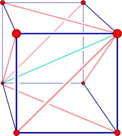
Figure 1: The cubic lattice, corresponding to the trajectory in moduli space given in eq. (4.34).

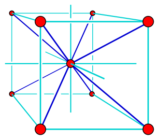
Figure 2: The $A_{3}^{*}$ lattice corresponding to the trajectory eq. (4.35). The eight nearest neighbor links (dark blue) emanating from the central site may be associated with the eight 3-vectors $\pm{\bf e}_{m}$. The six second-nearest-neighbor links (light blue) correspond to the six 3-vectors $\pm{\bf w}_{k}$ in eq. (4.39).

The site ${\bf n}$ is identified with the spacetime location

$${\bf R}=a\sum_{\nu=1}^{3}({\boldsymbol{\mu}}_{\nu}\cdot{\bf n}){\bf e}_{\nu}$$ (159)

and a lattice displacement of one unit in direction ${\boldsymbol{\mu}}_{m}$ corresponds to a spacetime translation $a{\bf e}_{m}$. It is easy to see that each of the four links occupied by four $z^{m}$ variables has length $|a{\bf e}_{m}|=\sqrt{\frac{3}{4}}\,a$, unlike the case of the less symmetric cubic lattice where $z^{4}$ resides on a link $\sqrt{3}$ times longer then the ones occupied by the three $z^{m}$.

A picture of the lattice is shown in Fig. 2. The dark blue links between nearest neighbor sites correspond to the eight 3-vectors $\pm{\bf e}_{m}$. It is helpful to also define the three orthonormal vectors

$${\bf w}_{k}\equiv{\bf e}_{4}+{\bf e}_{k}\ ,\qquad{\bf w}_{i}\cdot{\bf w}_{j}=\delta_{ij}\ ,\qquad i,j,k=1,\ldots,3\ .$$ (160)

The six $\pm{\bf w}_{k}$ vectors correspond to the light blue links between second nearest neighbors in Fig. 2. The $\mathbf{Z}^{m}$ and $\kern 0.6pt\overline{\kern-0.6pt\mathbf{Z}\kern-0.6pt}\kern 0.6pt_{m}$ superfields reside on the dark blue links; the $\boldsymbol{\Xi}^{k}$ and $\kern 0.6pt\overline{\kern-0.6pt\boldsymbol{\Xi}\kern-0.6pt}\kern 0.6pt_{k}$ superfields live on the light blue links, and the $\bf T$ and $\bf\Upsilon$ superfields live on the sites. However one should note that the superfields are not completely local, and contain terms looking like the square root of a plaquette.

In order to relate the lattice fields to continuum fields, we expand the lattice action around the point eq. (153). However, the structure of the lattice is dictated by $SU(4)\times U(1)\times U(1)$ and the continuum fields transform under $SO(3)\times SO(7)$. To make the connection between lattice and continuum fields clear, we introduce a $4\times 4$ real orthogonal matrix

$${\cal E}=\begin{pmatrix}\ \ \frac{1}{\sqrt{2}}&\ \ \frac{1}{\sqrt{6}}&\ \ \frac{1}{\sqrt{12}}&\ \ \frac{1}{2}\cr-\frac{1}{\sqrt{2}}&\ \ \frac{1}{\sqrt{6}}&\ \ \frac{1}{\sqrt{12}}&\ \ \frac{1}{2}\cr\ \ 0&-\frac{2}{\sqrt{6}}&\ \ \frac{1}{\sqrt{12}}&\ \ \frac{1}{2}\cr\ \ 0&\ \ 0&-\frac{3}{\sqrt{12}}&\ \ \frac{1}{2}\end{pmatrix}=\left({\cal E}^{T}\right)^{-1}$$ (161)

Note that ${\cal E}_{m\mu}$, with $\mu=1,\ldots 3$, are the components of the vectors ${\bf e}_{m}$ of eq. (157). This matrix has the property that

$$\left(\sum_{m=1}^{4}{\bf e}_{m}\,{\cal E}_{mn}\right)_{\mu}=\begin{cases}\delta_{n\mu}&n=1,\ldots,3\cr 0&n=4\ .\end{cases}$$ (162)

which serves as a bridge between the $SU(4)$ tensors of the lattice construction, and the $SO(3)$ representations of the continuum theory. In terms of this matrix we then define the expansion of $z^{m}$ about the point in moduli space eq. (153) to be

$$z^{m}=\frac{1}{a\sqrt{2}}+\sum_{m=1}^{4}{\cal E}_{mn}\Phi_{n}=\frac{1}{a\sqrt{2}}+\sum_{\mu=1}^{3}({\bf e}_{m})_{\mu}\Phi_{\mu}+\frac{1}{2}\Phi_{4}\ ,$$ (163)

with

$$\Phi_{\mu}\equiv\left(\frac{S_{\mu}+iV_{\mu}}{\sqrt{2}}\right)\ ,\quad\mu=1,\ldots,3\ ,\qquad\Phi_{4}\equiv\left(\frac{S_{4}+iS_{5}}{\sqrt{2}}\right)\ ,\qquad t\equiv\left(\frac{S_{6}+iS_{7}}{\sqrt{2}}\right)\ \$$ (164)

where $V_{\mu}$ and $S_{i}$ are hermitean $k\times k$ matrices, corresponding to gauge fields and scalars of the continuum theory.

We now will expand the action eq. (LABEL:eq:d3lat) to leading order in powers of the lattice spacing $a$, with the goal to show the equivalence in the continuum limit at tree level between our lattice action and the target theory action. Since the Jacobian of the transformation between lattice coordinates ${\bf n}$ and spacetime coordinates ${\bf R}$ in eq. (159) equals $a^{3}/2$, we first must rescale our coupling $g$ such that

$$\frac{1}{g^{2}}=\frac{a^{3}}{2\,g_{3}^{2}}\ ,\qquad\lim_{a\to 0}\frac{1}{g^{2}}\sum_{{\bf n}}=\frac{1}{g_{3}^{2}}\int d^{3}{\bf R}\ .$$ (165)

The analysis of the bosonic action of the lattice theory follows similarly to 3.5. None of the three types of bosonic terms are individually $SO(3)\times SO(7)$ invariant. However, upon adding them one gets the bosonic part of the target theory action,

$$S_{\text{boson}}=\frac{1}{g_{3}^{2}}\int d^{3}{\bf R}\,\operatorname{Tr\,}\,\left[\frac{1}{2}(D_{\mu}S_{a})^{2}+\frac{1}{4}V_{\mu\nu}^{2}-\frac{1}{4}[S_{a},S_{b}]^{2}\right]+O(a)\ ,$$ (166)

where in this section the indices $a,b=1,\ldots,7$ are $SO(7)$ indices, while $\mu,\nu=1,\ldots,3$ are spacetime indices. Notice that in this theory, two out of seven scalar arises from the site fields, whereas the other five scalar fields arise from the link variables transforming nontrivially under the lattice symmetries, yet they become in scalars under the $SO(3)$ spacetime rotations, transforming instead under the independent $SO(7)$ global $R$-symmetry that emerges in the continuum.

Similar to the analysis of fermionic terms in § 3.5, we can express the continuum limit of the fermion action eq. (LABEL:eq:d3lat) in terms of $\tilde{\omega}$ as

$$S_{\text{f}} = \frac{1}{g_{3}^{2}}\int d^{3}{\bf R}\,\operatorname{Tr\,}\,\frac{1}{2}\,\tilde{\omega}^{T}{\cal C}\,\bigl{(}\Gamma_{m}\,{\cal E}_{m\mu}D_{\mu}\tilde{\omega}+i\,\Gamma_{m+5}\,{\cal E}_{mn}[S_{n},\tilde{\omega}]+i\Gamma_{m}\,{\cal E}_{m4}[S_{5},\tilde{\omega}]$$ (168)

$$+i\Gamma_{10}\,[S_{6},\tilde{\omega}]+i\Gamma_{5}\,[S_{7},\tilde{\omega}]\bigr{)}$$

where the $\Gamma_{\alpha}$ are $SO(10)$ gamma matrices in the basis used to define the mother theory, eq. (6). Since ${\cal E}$ is an orthogonal matrix, we can define a new gamma matrix basis for $SO(10)$

$$\tilde{\Gamma}_{\mu}=\Gamma_{m}\,{\cal E}_{m\mu}\ ,\ \ \tilde{\Gamma}_{n+3}=\Gamma_{m+5}\,{\cal E}_{mn}\ ,\ \ \tilde{\Gamma}_{8}=\Gamma_{m}\,{\cal E}_{m4}\ ,\ \ \tilde{\Gamma}_{9}=\Gamma_{10}\ ,\ \ \tilde{\Gamma}_{10}=\Gamma_{5}\,\ .$$ (170)

In the new basis the charge conjugation matrix is unchanged, $\tilde{\cal C}={\cal C}$, given that we specified in eq. (4) that the $\Gamma_{m}$ be antisymmetric for $m=1,\ldots,5$ and symmetric for $m=6,\ldots,10$. Therefore, the above continuum limit of the lattice fermion action may be written as

$$S_{\text{fermion}} = \frac{1}{g_{3}^{2}}\int d^{3}{\bf R}\ \frac{1}{2}\,\operatorname{Tr\,}\,\Bigl{(}\tilde{\omega}^{T}\tilde{\cal C}\,\tilde{\Gamma}_{\mu}D_{\mu}\tilde{\omega}+i\,\tilde{\omega}^{T}\,\tilde{\cal C}\,\tilde{\Gamma}_{3+i}\,[S_{i},\tilde{\omega}]\Bigr{)}+O(a)$$ (171)

where the index $\mu$ is over $1\ldots 3$ and $i$ is over $1\ldots 7$. The chiral symmetry of the theory, $SO(7)$, which does not exist for any finite lattice spacing, emerged naturally in the continuum.

In conclusion, our construction of $A^{*}_{3}$ lattice with ${\cal Q}=2$ supersymmetry correctly reproduce the sixteen supercharge (${\cal N}=8$) SYM theory in $d=3$ dimensions. The discrete and continuous symmetries on the lattice, $S_{4}\ltimes Z_{2}\times(U(1)\times U(1))$ enhances to $SO(3)\times SO(7)$ symmetry in the continuum.

5 The two dimensional lattice

5.1 The mother theory with manifest ${\cal Q}=4$ supersymmetry in $SU(3)\times U(1)\times SO(4)$ multiplets

We now turn to the sixteen supercharge target theory in two dimensions, also known as ${\cal N}=(8,8)$ supersymmetry, which possesses an $SO(8)$ $R$-symmetry. In this case the lattice possesses four exact supercharges, and the multiplet structure is identical to that of the familiar ${\cal N}=1$ supersymmetric gauge theories in four dimensions, and we can use superfields reduced from four dimensions to describe the theory. Here we give an abbreviated version of the analysis, trusting that familiarity with the previous two sections of this paper will make it straight forward to fill in the missing details.

To create a two dimensional lattice, we orbifold the mother theory eq. (6) by a $Z_{N}\times Z_{N}$ symmetry. The two dimensional ${\bf r}$ charges generate the Cartan algebra of an $SU(3)$ subgroup of $SO(10)$ embedded in the natural way along the chain $SO(10)\to SO(4)\times SO(6)\to SO(4)\times SU(3)\times U(1)$. The $SO(4)\times U(1)\simeq SU(2)\times SU(2)\times U(1)$ symmetry will remain exact on the lattice, while the $SU(3)$ symmetry is broken to $U(1)\times U(1)$, by the orbifold projection, with fields assigned to links and sites according to their $SU(3)$ weights.

The ten bosons and the sixteen fermions of the mother theory decompose under the $SU(3)\times SU(2)\times SU(2)\times U(1)$ subgroup of $SO(10)$ as

$$v\sim{\bf 10}\ \longrightarrow\ z\oplus\kern 0.6pt\overline{\kern-0.6ptz\kern-0.6pt}\kern 0.6pt\oplus\tilde{v}\sim({\bf 3,1,1})_{\bf 1}\oplus({\bf\kern 0.6pt\overline{\kern-0.6pt3\kern-0.6pt}\kern 0.6pt,1,1})_{-{\bf 1}}\oplus({\bf 1,2,2})_{\bf 0}\ .$$ (173)

$$\omega\sim{\bf 16}\ \longrightarrow\ \psi\oplus\kern 0.6pt\overline{\kern-0.6pt\psi\kern-0.6pt}\kern 0.6pt\oplus\lambda\oplus\kern 0.6pt\overline{\kern-0.6pt\lambda\kern-0.6pt}\kern 0.6pt\sim({\bf 3,2,1})_{-\frac{\bf 1}{{\bf 2}}}\oplus({\bf\kern 0.6pt\overline{\kern-0.6pt3\kern-0.6pt}\kern 0.6pt,1,2})_{\frac{\bf 1}{{\bf 2}}}\oplus({\bf 1,2,1})_{\frac{\bf 3}{{\bf 2}}}\oplus({\bf 1,1,2})_{-\frac{\bf 3}{{\bf 2}}}\ \$$ (174)

The fermions are now doublets under the $SU(2)\times SU(2)$ symmetry, and we adopt the conventions of Wess and Bagger [32] adapted for Euclidean spacetime (see Appendix C). For a more explicit discussion of the above decomposition, see Appendix D.

After orbifolding, the location on the lattice of the above variables is determined as before by the ${\bf r}$ charges, as given in Table 3. We see that $\tilde{v}$ and $\lambda$ are site variables, while $z^{m}$, $\psi^{m}$, $\kern 0.6pt\overline{\kern-0.6ptz\kern-0.6pt}\kern 0.6pt_{m}$ and $\kern 0.6pt\overline{\kern-0.6pt\psi\kern-0.6pt}\kern 0.6pt_{m}$ are link variables, where the links are designated by ${\bf r}$ equaling one of the three vectors

$$\boldsymbol{\mu}_{1} = \{1,0\}\ ,$$ (175)

$$\boldsymbol{\mu}_{2} = \{0,1\}\,$$ (176)

$$\boldsymbol{\mu}_{3} = \{-1,-1\}\ .$$ (177)

	$SU(2)\times SU(2)\times U(1)$	$q_{1}\$	$q_{2}\$	$q_{3}\$		r
$z^{1}$	$({\bf 1,1})_{\bf 1}$	$\,\ 1$	$\,\ 0$	$\,\ 0$	$\{1,0\}$	=	$\ \ \boldsymbol{\mu}_{1}$
$z^{2}$	$({\bf 1,1})_{\bf 1}$	$\,\ 0$	$\,\ 1$	$\,\ 0$	$\{0,1\}$	=	$\ \ \boldsymbol{\mu}_{2}$
$z^{3}$	$({\bf 1,1})_{\bf 1}$	$\,\ 0$	$\,\ 0$	$\,\ 1$	$\{-1,-1\}$	=	$\ \ \boldsymbol{\mu}_{3}$
$\kern 0.6pt\overline{\kern-0.6ptz\kern-0.6pt}\kern 0.6pt_{1}$	$({\bf 1,1})_{\bf-1}$	$\,\ -1$	$\,\ 0$	$\,\ 0$	$\{-1,0\}$	=	$-\boldsymbol{\mu}_{1}$
$\kern 0.6pt\overline{\kern-0.6ptz\kern-0.6pt}\kern 0.6pt_{2}$	$({\bf 1,1})_{\bf-1}$	$\,\ 0$	$\,\ -1$	$\,\ 0$	$\{0,-1\}$	=	$-\boldsymbol{\mu}_{2}$
$\kern 0.6pt\overline{\kern-0.6ptz\kern-0.6pt}\kern 0.6pt_{3}$	$({\bf 1,1})_{\bf-1}$	$\,\ 0$	$\,\ 0$	$\,\ -1$	$\{1,1\}$	=	$-\boldsymbol{\mu}_{3}$
$\tilde{v}$	$({\bf 2,2})_{\bf 0}$	$\,\ 0$	$\,\ 0$	$\,\ 0$	$\{0,0\}$	=	0
$\lambda$	$({\bf 2,1})_{\bf\frac{3}{2}}$	$\ {\textstyle{\frac{1}{2}}}$	$\ {\textstyle{\frac{1}{2}}}$	$\ {\textstyle{\frac{1}{2}}}$	$\{0,0\}$	=	0
$\kern 0.6pt\overline{\kern-0.6pt\lambda\kern-0.6pt}\kern 0.6pt$	$({\bf 1,2})_{\bf-\frac{3}{2}}$	$-{\textstyle{\frac{1}{2}}}$	$-{\textstyle{\frac{1}{2}}}$	$-{\textstyle{\frac{1}{2}}}$	$\{0,0\}$	=	0
$\psi^{1}$	$({\bf 2,1})_{\bf-\frac{1}{2}}$	$\ {\textstyle{\frac{1}{2}}}$	$-{\textstyle{\frac{1}{2}}}$	$-{\textstyle{\frac{1}{2}}}$	$\{1,0\}$	=	$\ \ \boldsymbol{\mu}_{1}$
$\psi^{2}$	$({\bf 2,1})_{\bf-\frac{1}{2}}$	$-{\textstyle{\frac{1}{2}}}$	$\ {\textstyle{\frac{1}{2}}}$	$-{\textstyle{\frac{1}{2}}}$	$\{0,1\}$	=	$\ \ \boldsymbol{\mu}_{2}$
$\psi^{3}$	$({\bf 2,1})_{\bf-\frac{1}{2}}$	$-{\textstyle{\frac{1}{2}}}$	$-{\textstyle{\frac{1}{2}}}$	$\ {\textstyle{\frac{1}{2}}}$	$\{-1,-1\}$	=	$\ \ \boldsymbol{\mu}_{3}$
$\kern 0.6pt\overline{\kern-0.6pt\psi\kern-0.6pt}\kern 0.6pt_{1}$	$({\bf 1,2})_{\bf\frac{1}{2}}$	$-{\textstyle{\frac{1}{2}}}$	$\ {\textstyle{\frac{1}{2}}}$	$\ {\textstyle{\frac{1}{2}}}$	$\{-1,0\}$	=	$-\boldsymbol{\mu}_{1}$
$\kern 0.6pt\overline{\kern-0.6pt\psi\kern-0.6pt}\kern 0.6pt_{2}$	$({\bf 1,2})_{\bf\frac{1}{2}}$	$\ {\textstyle{\frac{1}{2}}}$	$-{\textstyle{\frac{1}{2}}}$	$\ {\textstyle{\frac{1}{2}}}$	$\{0,-1\}$	=	$-\boldsymbol{\mu}_{2}$
$\kern 0.6pt\overline{\kern-0.6pt\psi\kern-0.6pt}\kern 0.6pt_{3}$	$({\bf 1,2})_{\bf\frac{1}{2}}$	$\ {\textstyle{\frac{1}{2}}}$	$\ {\textstyle{\frac{1}{2}}}$	$-{\textstyle{\frac{1}{2}}}$	$\{1,1\}$	=	$-\boldsymbol{\mu}_{3}$

Table 3: The $SU(2)\times SU(2)\times U(1)$, ${q_{m}}$ and $r_{\mu}=(q_{\mu}-q_{3})$ representations of the bosonic variables $v$ and fermionic variables $\omega$ of the ${\cal Q}=16$ mother theory under the $SO(10)\supset SU(3)\times SU(2)\times SU(2)\times U(1)$ decomposition.

The mother theory may be most easily expressed in a manifestly ${\cal Q}=4$ supersymmetric form by writing the ${\cal N}=4$ SYM in four dimensions using ${\cal N}=1$ superfields, and then dimensionally reducing to zero dimensions. The result is the action

$$S = \frac{1}{g^{2}}\operatorname{Tr\,}\biggl{[}\int d^{2}\theta\;d^{2}\kern 0.6pt\overline{\kern-0.6pt\theta\kern-0.6pt}\kern 0.6pt\;\;\kern 0.6pt\overline{\kern-0.6pt\mathbf{Z}\kern-0.6pt}\kern 0.6pt_{m}e^{2{\bf V}}{\mathbf{Z}}^{m}e^{-2{\bf V}}+\;\frac{1}{4}\int d^{2}\theta\;{\bf W}^{\alpha}{\bf W}_{\alpha}+\frac{1}{4}\int d^{2}{\kern 0.6pt\overline{\kern-0.6pt\theta\kern-0.6pt}\kern 0.6pt}\;\kern 0.6pt\overline{\kern-0.6pt\bf W\kern-0.6pt}\kern 0.6pt_{{\dot{\alpha}}}\kern 0.6pt\overline{\kern-0.6pt\bf W\kern-0.6pt}\kern 0.6pt^{{\dot{\alpha}}}$$

$$+ \frac{\sqrt{2}}{3!}\epsilon_{mnp}\int d^{2}\theta\,{\mathbf{Z}}^{m}[\mathbf{Z}^{n},\mathbf{Z}^{p}]-\frac{\sqrt{2}}{3!}\epsilon^{mnp}\int d^{2}\kern 0.6pt\overline{\kern-0.6pt\theta\kern-0.6pt}\kern 0.6pt\,\kern 0.6pt\overline{\kern-0.6pt\mathbf{Z}\kern-0.6pt}\kern 0.6pt_{m}[\kern 0.6pt\overline{\kern-0.6pt\mathbf{Z}\kern-0.6pt}\kern 0.6pt_{n},\kern 0.6pt\overline{\kern-0.6pt\mathbf{Z}\kern-0.6pt}\kern 0.6pt_{p}]\biggr{]}$$

where $\mathbf{Z}^{m}$ and $\kern 0.6pt\overline{\kern-0.6pt\mathbf{Z}\kern-0.6pt}\kern 0.6pt_{m}$ are chiral and anti-chiral superfields respectively, and ${\bf V}$ is a vector multiplet, expanded in components as

$$\mathbf{Z}^{m} = z^{m}+\sqrt{2}\theta\psi^{m}+\theta\theta F^{m}$$ (179)

$${\kern 0.6pt\overline{\kern-0.6pt\mathbf{Z}\kern-0.6pt}\kern 0.6pt}_{m} = \kern 0.6pt\overline{\kern-0.6ptz\kern-0.6pt}\kern 0.6pt_{m}+\sqrt{2}\kern 0.6pt\overline{\kern-0.6pt\theta\kern-0.6pt}\kern 0.6pt\kern 0.6pt\overline{\kern-0.6pt\psi\kern-0.6pt}\kern 0.6pt_{m}+\kern 0.6pt\overline{\kern-0.6pt\theta\kern-0.6pt}\kern 0.6pt\kern 0.6pt\overline{\kern-0.6pt\theta\kern-0.6pt}\kern 0.6pt\kern 0.6pt\overline{\kern-0.6ptF\kern-0.6pt}\kern 0.6pt_{m}$$ (180)

$${\bf V} = -\theta\sigma_{a}\tilde{v}_{a}\kern 0.6pt\overline{\kern-0.6pt\theta\kern-0.6pt}\kern 0.6pt+\theta\theta\kern 0.6pt\overline{\kern-0.6pt\theta\kern-0.6pt}\kern 0.6pt\kern 0.6pt\overline{\kern-0.6pt\lambda\kern-0.6pt}\kern 0.6pt+\kern 0.6pt\overline{\kern-0.6pt\theta\kern-0.6pt}\kern 0.6pt\kern 0.6pt\overline{\kern-0.6pt\theta\kern-0.6pt}\kern 0.6pt\theta\lambda+{\textstyle{\frac{1}{2}}}\theta\theta\kern 0.6pt\overline{\kern-0.6pt\theta\kern-0.6pt}\kern 0.6pt\kern 0.6pt\overline{\kern-0.6pt\theta\kern-0.6pt}\kern 0.6pt\,d$$ (181)

$${\bf W}_{\alpha} = -\lambda_{\alpha}+(-(\sigma_{ab}v_{ab})_{\alpha}^{\ \ \beta}+\delta_{\alpha}^{\beta}d)\theta_{\beta}-\theta\theta(\sigma_{a})_{\alpha\dot{\beta}}[v_{a},\kern 0.6pt\overline{\kern-0.6pt\lambda\kern-0.6pt}\kern 0.6pt^{\dot{\beta}}]$$ (182)

$${\bf W}^{\dot{\alpha}} = -\kern 0.6pt\overline{\kern-0.6pt\lambda\kern-0.6pt}\kern 0.6pt^{\dot{\alpha}}+((\kern 0.6pt\overline{\kern-0.6pt\sigma\kern-0.6pt}\kern 0.6pt_{ab}v_{ab})^{\dot{\alpha}}_{\ \ \dot{\beta}}+\delta^{\dot{\alpha}}_{\dot{\beta}}d)\kern 0.6pt\overline{\kern-0.6pt\theta\kern-0.6pt}\kern 0.6pt^{\dot{\beta}}-\kern 0.6pt\overline{\kern-0.6pt\theta\kern-0.6pt}\kern 0.6pt\kern 0.6pt\overline{\kern-0.6pt\theta\kern-0.6pt}\kern 0.6pt(\kern 0.6pt\overline{\kern-0.6pt\sigma\kern-0.6pt}\kern 0.6pt_{a})^{\dot{\alpha}\beta}[v_{a},\lambda_{\beta}].$$ (183)

The ${\bf W}_{\alpha}$ and $\kern 0.6pt\overline{\kern-0.6pt\bf W\kern-0.6pt}\kern 0.6pt_{{\dot{\alpha}}}$ are the usual spinorial field strength chiral superfields that give rise in four dimensions to the kinetic terms for the gauge bosons and gauginos.

The off-shell supersymmetric variations of these components in terms of the four Grassmann parameters $\zeta$ and $\kern 0.6pt\overline{\kern-0.6pt\zeta\kern-0.6pt}\kern 0.6pt$ (transforming as $(2,1)$ and $(1,2)$ respectively under $SU(2)\times SU(2)$) are given by

$$\delta z^{m} = \sqrt{2}i\zeta\psi^{m},\qquad$$ (184)

$$\delta{\kern 0.6pt\overline{\kern-0.6ptz\kern-0.6pt}\kern 0.6pt}_{m} = -\sqrt{2}i{\kern 0.6pt\overline{\kern-0.6pt\zeta\kern-0.6pt}\kern 0.6pt}{\kern 0.6pt\overline{\kern-0.6pt\psi\kern-0.6pt}\kern 0.6pt}_{m}$$ (185)

$$\delta\psi^{m} = +\sqrt{2}i(\sigma_{a}){\kern 0.6pt\overline{\kern-0.6pt\zeta\kern-0.6pt}\kern 0.6pt}[\tilde{v}_{a},z^{m}]+\sqrt{2}i\zeta F^{m}$$ (186)

$$\delta{\kern 0.6pt\overline{\kern-0.6pt\psi\kern-0.6pt}\kern 0.6pt}_{m} = -\sqrt{2}i({\kern 0.6pt\overline{\kern-0.6pt\sigma\kern-0.6pt}\kern 0.6pt}_{a}){\zeta}[\tilde{v}_{a},{\kern 0.6pt\overline{\kern-0.6ptz\kern-0.6pt}\kern 0.6pt_{m}}]-\sqrt{2}i\kern 0.6pt\overline{\kern-0.6pt\zeta\kern-0.6pt}\kern 0.6pt{\kern 0.6pt\overline{\kern-0.6ptF\kern-0.6pt}\kern 0.6pt}_{m}$$ (187)

$$\delta\tilde{v}_{a} = +i\kern 0.6pt\overline{\kern-0.6pt\lambda\kern-0.6pt}\kern 0.6pt\kern 0.6pt\overline{\kern-0.6pt\sigma\kern-0.6pt}\kern 0.6pt_{a}\zeta-i{\kern 0.6pt\overline{\kern-0.6pt\zeta\kern-0.6pt}\kern 0.6pt}{\kern 0.6pt\overline{\kern-0.6pt\sigma\kern-0.6pt}\kern 0.6pt}_{a}\lambda$$ (188)

$$\delta\lambda = -i({\sigma}_{ab}\tilde{v}_{ab})\zeta+i\zeta d$$ (189)

$$\delta\kern 0.6pt\overline{\kern-0.6pt\lambda\kern-0.6pt}\kern 0.6pt = -i({\kern 0.6pt\overline{\kern-0.6pt\sigma\kern-0.6pt}\kern 0.6pt}_{ab}\tilde{v}_{ab})\kern 0.6pt\overline{\kern-0.6pt\zeta\kern-0.6pt}\kern 0.6pt-i\kern 0.6pt\overline{\kern-0.6pt\zeta\kern-0.6pt}\kern 0.6ptd$$ (190)

$$\delta d = i\zeta\sigma_{a}[\tilde{v}_{a},\kern 0.6pt\overline{\kern-0.6pt\lambda\kern-0.6pt}\kern 0.6pt]+i[\tilde{v}_{a},\lambda]\sigma_{a}\kern 0.6pt\overline{\kern-0.6pt\zeta\kern-0.6pt}\kern 0.6pt\$$ (191)

$$\delta F^{m} = -i\sqrt{2}\kern 0.6pt\overline{\kern-0.6pt\zeta\kern-0.6pt}\kern 0.6pt\kern 0.6pt\overline{\kern-0.6pt\sigma\kern-0.6pt}\kern 0.6pt_{a}[\tilde{v}_{a},\psi^{m}]+2i[z^{m},\kern 0.6pt\overline{\kern-0.6pt\lambda\kern-0.6pt}\kern 0.6pt]\kern 0.6pt\overline{\kern-0.6pt\zeta\kern-0.6pt}\kern 0.6pt$$ (192)

$$\delta\kern 0.6pt\overline{\kern-0.6ptF\kern-0.6pt}\kern 0.6pt_{m} = -i\sqrt{2}\zeta\sigma_{a}[\tilde{v}_{a},\kern 0.6pt\overline{\kern-0.6pt\psi\kern-0.6pt}\kern 0.6pt_{m}]+2i[\kern 0.6pt\overline{\kern-0.6ptz\kern-0.6pt}\kern 0.6pt_{m},\lambda]\zeta\ .$$ (193)

where the auxiliary fields satisfy the equations of motion

$$d = -[\kern 0.6pt\overline{\kern-0.6ptz\kern-0.6pt}\kern 0.6pt_{m},z^{m}]\ ,$$ (194)

$$F^{m} = -\frac{1}{\sqrt{2}}\epsilon^{mnp}[\kern 0.6pt\overline{\kern-0.6ptz\kern-0.6pt}\kern 0.6pt_{n},\kern 0.6pt\overline{\kern-0.6ptz\kern-0.6pt}\kern 0.6pt_{p}]$$ (195)

$$\kern 0.6pt\overline{\kern-0.6ptF\kern-0.6pt}\kern 0.6pt_{m} = +\frac{1}{\sqrt{2}}\epsilon_{mnp}[z^{n},z^{p}]\ .$$ (196)

5.2 The $d=2$, ${\cal Q}=4$ lattice theory

The steps for constructing the $d=2$, ${\cal Q}=4$ lattice for the $(8,8)$ target theory are similar to those followed in previous sections. After the $Z_{N}\times Z_{N}$ orbifold projection of the mother theory, one obtains the lattice action, written with manifest ${\cal Q}=4$ supersymmetry

$$S= \frac{1}{g^{2}}\sum_{{\bf n}}\operatorname{Tr\,}\biggl{[}\int d^{2}\theta\;d^{2}\kern 0.6pt\overline{\kern-0.6pt\theta\kern-0.6pt}\kern 0.6pt\;\;\kern 0.6pt\overline{\kern-0.6pt\mathbf{Z}\kern-0.6pt}\kern 0.6pt_{m}({\bf n})e^{2{\bf V}({{\bf n}})}{\mathbf{Z}}^{m}({\bf n})e^{-2{\bf V}({\bf n}+\boldsymbol{\mu}_{m})}$$ (197)

$$+\;\frac{1}{4}\int d^{2}\theta\;{\bf W}^{\alpha}({\bf n}){\bf W}_{\alpha}({\bf n})+\frac{1}{4}\int d^{2}{\kern 0.6pt\overline{\kern-0.6pt\theta\kern-0.6pt}\kern 0.6pt}\;\kern 0.6pt\overline{\kern-0.6pt\bf W\kern-0.6pt}\kern 0.6pt_{{\dot{\alpha}}}({\bf n})\kern 0.6pt\overline{\kern-0.6pt\bf W\kern-0.6pt}\kern 0.6pt^{{\dot{\alpha}}}({{\bf n}})$$

$$+\frac{\sqrt{2}}{3!}\epsilon_{mnp}\int d^{2}\theta\,{\mathbf{Z}}^{m}({\bf n})(\mathbf{Z}^{n}({\bf n}+\boldsymbol{\mu}_{m})\mathbf{Z}^{p}({\bf n}-\boldsymbol{\mu}_{p})-\mathbf{Z}^{p}({\bf n}+\boldsymbol{\mu}_{m})\mathbf{Z}_{n}({\bf n}-\boldsymbol{\mu}_{n}))$$

$$+\frac{\sqrt{2}}{3!}\epsilon^{mnp}\int d^{2}\kern 0.6pt\overline{\kern-0.6pt\theta\kern-0.6pt}\kern 0.6pt\,\kern 0.6pt\overline{\kern-0.6pt\mathbf{Z}\kern-0.6pt}\kern 0.6pt_{m}({\bf n})(\kern 0.6pt\overline{\kern-0.6pt\mathbf{Z}\kern-0.6pt}\kern 0.6pt_{n}({\bf n}-\boldsymbol{\mu}_{n})\kern 0.6pt\overline{\kern-0.6pt\mathbf{Z}\kern-0.6pt}\kern 0.6pt_{p}({\bf n}+\boldsymbol{\mu}_{m})-\kern 0.6pt\overline{\kern-0.6pt\mathbf{Z}\kern-0.6pt}\kern 0.6pt_{p}({\bf n}-\boldsymbol{\mu}_{p})\kern 0.6pt\overline{\kern-0.6pt\mathbf{Z}\kern-0.6pt}\kern 0.6pt_{n}({\bf n}+\boldsymbol{\mu}_{m}))\biggr{]}$$

One then expands the theory about a particular trajectory in moduli space. For a square lattice, the expansion is about

$$z^{m}({\bf n})=\kern 0.6pt\overline{\kern-0.6ptz\kern-0.6pt}\kern 0.6pt_{m}({\bf n})=\frac{1}{a{\sqrt{2}}}{\bf 1}_{k},\,\,\,m=1\ldots 2,\qquad z^{3}({\bf n})=\kern 0.6pt\overline{\kern-0.6ptz\kern-0.6pt}\kern 0.6pt_{3}({\bf n})=0.$$ (198)

With this choice $\boldsymbol{\mu}_{1}$, $\boldsymbol{\mu}_{2}$ and $\boldsymbol{\mu}_{3}$ get mapped to the lattice vectors $\hat{\bf x}$, $\hat{\bf y}$ and $-(\hat{\bf x}+\hat{\bf y})$ respectively, and the lattice appears as in Fig. 4. A more symmetric alternative is the expansion about

$$z_{m}({\bf n})=\kern 0.6pt\overline{\kern-0.6ptz\kern-0.6pt}\kern 0.6pt^{m}({\bf n})=\frac{1}{a{\sqrt{2}}}{\bf 1}_{k},\,\,\,m=1\ldots 3,$$ (199)

which treats all bosonic link fields on equal footing and gives rise to the $A_{2}^{*}$ (triangular) lattice shown in Fig. 4.

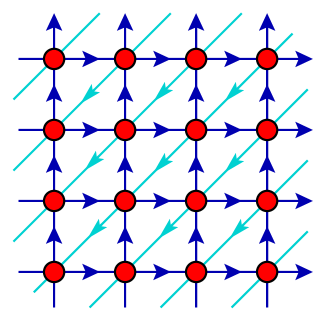
Figure 3: The square $d=2$ lattice following from the expansion eq. (5.9). The ${\bf r}=\boldsymbol{\mu}_{1,2}$ variables in Table 3. reside on the $\hat{\bf x}$ and $\hat{\bf y}$ links respectively, while charge ${\bf r}=\boldsymbol{\mu}_{3}$ maps variables onto the diagonal links; $\tilde{v}$ and $\lambda$, $\kern 0.6pt\overline{\kern-0.6pt\lambda\kern-0.6pt}\kern 0.6pt$ have ${\bf r}={\bf 0}$ and reside at the sites.

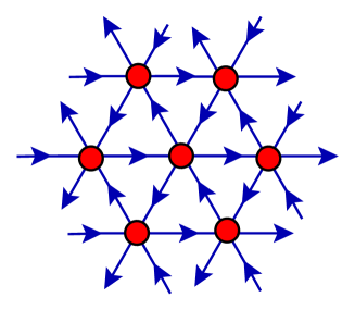
Figure 4: The triangular $d=2$ lattice ($A_{2}^{*}$) corresponding to expansion about the symmetric point in moduli space, eq. (5.10). The ${\bf r}=\pm\boldsymbol{\mu}_{m}$ variables $z^{m}$, $\kern 0.6pt\overline{\kern-0.6ptz\kern-0.6pt}\kern 0.6pt_{m}$, $\psi^{m}$ and $\kern 0.6pt\overline{\kern-0.6pt\psi\kern-0.6pt}\kern 0.6pt_{m}$ reside on the links, while $\tilde{v}$ and $\lambda$, $\kern 0.6pt\overline{\kern-0.6pt\lambda\kern-0.6pt}\kern 0.6pt$ have ${\bf r}={\bf 0}$ and reside at the sites.

To analyze the continuum limit of the $A_{2}^{*}$ lattice, we introduce three two dimensional vectors to relate the point ${\bf n}$ to a spacetime point. These lattice vectors can be chosen as

$${\bf e_{1}} = (\frac{1}{\sqrt{2}},\frac{1}{\sqrt{6}})\ ,$$ (200)

$${\bf e_{2}} = (-\frac{1}{\sqrt{2}},\frac{1}{\sqrt{6}})\ ,$$ (201)

$${\bf e_{3}} = (0,-\frac{2}{\sqrt{6}})\ ,$$ (202)

and satisfy the relations

$$\sum_{m=1}^{3}{\bf e}_{m}=0,\qquad{\bf e}_{m}\cdot{\bf e}_{n}=\delta_{mn}-{\textstyle{\frac{1}{3}}}\qquad\sum_{m=1}^{3}({\bf e}_{m})_{\mu}({\bf e}_{m})_{\nu}=\delta_{\mu\nu}$$ (203)

The lattice vectors are the $SU(3)$ weights of the $\bf 3$ representation, and they form a 2-simplex (equilateral triangle) in two dimensions. The matrix ${\bf e}_{m}\cdot{\bf e}_{n}$ is the Gram matrix of $A_{2}^{*}$ [30], also known as hexagonal lattice.

The site ${\bf n}$ is identified with the spacetime location

$${\bf R}=a\sum_{\nu=1}^{2}({\boldsymbol{\mu}}_{\nu}\cdot{\bf n}){\bf e}_{\nu}=$$ (204)

and a lattice displacement of one unit in direction ${\boldsymbol{\mu}}_{m}$ corresponds to a spacetime translation $a{\bf e}_{m}$. Each of the three links occupied by three $z^{m}$ variables has length $|a{\bf e}_{m}|=\sqrt{\frac{2}{3}}\,a$, unlike the case of the less symmetric square lattice where $z^{3}$ resides on a link $\sqrt{2}$ times longer then the ones occupied by the three $z^{m},\ m=1,2$.

In order to relate the lattice fields to continuum fields, we expand the lattice action around the point eq. (153). However, the structure of the lattice is dictated by $SU(3)$ and the continuum fields transform under $SO(2)\times SO(8)$ where $SO(2)$ Euclidean analog of the Lorentz symmetry and $SO(8)$ is the global R-symmetry. To make the connection between lattice and continuum fields, we introduce a $3\times 3$ real orthogonal matrix

$${\cal E}=\begin{pmatrix}\ \ \frac{1}{\sqrt{2}}&\ \ \frac{1}{\sqrt{6}}&\ \ \frac{1}{\sqrt{3}}\cr-\frac{1}{\sqrt{2}}&\ \ \frac{1}{\sqrt{6}}&\ \ \frac{1}{\sqrt{3}}\cr\ \ 0&-\frac{2}{\sqrt{6}}&\ \ \frac{1}{\sqrt{3}}\end{pmatrix}=\left({\cal E}^{T}\right)^{-1}$$ (205)

Note that ${\cal E}_{m\mu}$, with $\mu=1,2$, are the components of the vectors ${\bf e}_{m}$ of eq. (157). This matrix has the property that

$$\left(\sum_{m=1}^{3}{\bf e}_{m}\,{\cal E}_{mn}\right)_{\mu}=\begin{cases}\delta_{n\mu}&n=1,\ldots,2\cr 0&n=3\ .\end{cases}$$ (206)

which serves as a bridge between the $SU(3)$ tensors of the lattice construction, and the $SO(2)$ representations of the continuum theory. In terms of this matrix we then define the expansion of $z^{m}$ about the point in moduli space eq. (199) to be

$$z^{m}=\frac{1}{a\sqrt{2}}+\sum_{m=1}^{3}{\cal E}_{mn}\Phi_{n}=\frac{1}{a\sqrt{2}}+\sum_{\mu=1}^{2}({\bf e}_{m})_{\mu}\Phi_{\mu}+\frac{1}{\sqrt{3}}\Phi_{3}\ ,$$ (207)

with

$$\Phi_{\mu}\equiv\left(\frac{S_{\mu}+iV_{\mu}}{\sqrt{2}}\right),\ \mu=1,2\ ,\qquad\Phi_{3}\equiv\left(\frac{S_{3}+iS_{4}}{\sqrt{2}}\right),$$ (208)

and

$$\{\tilde{v}_{0},\tilde{v}_{1},\tilde{v}_{2},\tilde{v}_{3}\}\equiv\,\{S_{8},S_{5},S_{6},S_{7}\}\ .$$ (209)

where $V_{\mu}$ and $S_{a}$ are hermitean $k\times k$ matrices, corresponding to the two gauge fields and eight scalars of the continuum theory.

We expand the action eq. (197) to leading order in powers of the lattice spacing $a$ to obtain the continuum limit at tree level. Since the Jacobian of the transformation between lattice coordinates ${\bf n}$ and spacetime coordinates ${\bf R}$ in eq. (204) equals $a^{2}/\sqrt{3}$, we first must rescale our coupling $g$ such that

$$\frac{1}{g^{2}}=\frac{a^{2}}{\sqrt{3}\,g_{2}^{2}}\ ,\qquad\lim_{a\to 0}\frac{1}{g^{2}}\sum_{{\bf n}}=\frac{1}{g_{2}^{2}}\int d^{2}{\bf R}\ .$$ (210)

The analysis of the bosonic action of the lattice theory gives in the continuum $SO(2)\times SO(8)$ invariant action.

$$S_{\text{boson}}=\frac{1}{g_{2}^{2}}\int d^{2}{\bf R}\,\operatorname{Tr\,}\,\left[\frac{1}{2}(D_{\mu}S_{a})^{2}+\frac{1}{4}V_{\mu\nu}^{2}-\frac{1}{4}[S_{a},S_{b}]^{2}\right]+O(a)$$ (211)

where $\mu,\nu=1,2$ and $a,b=1\ldots 8$.

Similar to the analysis of fermionic terms in § 3.5, we can express the continuum limit of the fermion action eq. (197) in terms of $\tilde{\omega}$ as

$$S_{\text{fermion}} = \frac{1}{g_{2}^{2}}\int d^{2}{\bf R}\,\operatorname{Tr\,}\,\frac{1}{2}\,\tilde{\omega}^{T}{\cal C}\,\Bigl{(}\Gamma_{m}\,{\cal E}_{m\mu}D_{\mu}\tilde{\omega}+i\,\Gamma_{m+5}\,{\cal E}_{mn}[S_{n},\tilde{\omega}]+i\Gamma_{m}\,{\cal E}_{m3}[S_{4},\tilde{\omega}]$$ (213)

$$+i\sum_{i=1}^{2}\left(\Gamma_{11-i}\,[S_{2i+3},\tilde{\omega}]+\Gamma_{6-i}\,[S_{2i+4},\tilde{\omega}]\right)\Bigr{)}$$

where the $\Gamma_{\alpha}$ are $SO(10)$ gamma matrices in the basis used to define the mother theory, eq. (6). Since ${\cal E}$ is an orthogonal matrix, we can define a new gamma matrix basis for $SO(10)$

$$\tilde{\Gamma}_{\mu}=\Gamma_{m}\,{\cal E}_{m\mu}\ ,\ \ \tilde{\Gamma}_{n+2}=\Gamma_{m+5}\,{\cal E}_{mn}\ ,\ \ \tilde{\Gamma}_{6}=\Gamma_{m}\,{\cal E}_{m3},\ \$$ (214)

$$\tilde{\Gamma}_{2i+5}=\Gamma_{11-i}\ ,\ \ \tilde{\Gamma}_{2i+6}=\Gamma_{6-i}\ ,\qquad i=1,2\ .\$$

In the new basis the charge conjugation matrix is unchanged. Therefore, the above continuum limit of the lattice fermion action may be written as

$$S_{\text{fermion}} = \frac{1}{g_{2}^{2}}\int d^{2}{\bf R}\ \frac{1}{2}\,\operatorname{Tr\,}\,\Bigl{(}\tilde{\omega}^{T}\tilde{\cal C}\,\tilde{\Gamma}_{\mu}D_{\mu}\tilde{\omega}+i\,\tilde{\omega}^{T}\,\tilde{\cal C}\,\tilde{\Gamma}_{2+a}\,[S_{a},\tilde{\omega}]\Bigr{)}+O(a)\ .$$ (215)

The chiral symmetry of the theory, $SO(8)$, which does not exist for any finite lattice spacing, emerges naturally in the continuum. Combining $S_{\text{fermion}}+S_{\text{boson}}$ correctly reproduce the sixteen supercharge ${\cal N}=(8,8)$ SYM theory in $d=2$ dimensions.

6 The one dimensional lattice; or Euclidean path integrals for M-theory

The sixteen supercharge $U(N)$ matrix quantum mechanics is interesting because it has been argued that the large $N$ limit corresponds to $M$-theory [9]. Because of this limit, a Hamiltonian approach to the theory is not very practical (as one would expect for a theory that is supposed to contain higher dimensional physics), and so a path integral approach may prove to be more promising. Here we construct a version of the theory on a one-dimensional lattice in the Euclidean time direction, which possesses eight exact supersymmetries. The other eight appear in the continuum limit.

The theory continuum theory has a one-component gauge boson $V$ which is not dynamical, but which is rather a Lagrange multiplier. Integrating it out enforces the constraint on physical states that they be gauge invariant. The $R$-symmetry of the theory is $SO(9)$, under which the scalars transform as the ${\bf 9}$ dimensional vector representation and the fermions as the ${\bf 16}$ dimensional spinor representation. The action of the target theory is

$$S_{\text{target}}=\frac{1}{g_{1}^{2}}\,\int d{\tau}\,\operatorname{Tr\,}\Bigl{(}\frac{1}{2}(D_{\tau}S_{a})^{2}-\frac{1}{4}\left[S_{a},S_{b}\right]^{2}+\frac{1}{2}\tilde{\omega}^{T}\,\tilde{{\cal C}}\,D_{\tau}\,\tilde{\Gamma}_{1}\,\tilde{\omega}+\frac{i}{2}\,\tilde{\omega}^{T}\,\tilde{{\cal C}}\,\tilde{\Gamma}_{1+a}\,[S_{a},\tilde{\omega}]\Bigr{)}$$ (217)

(218)

where we introduced $SO(10)$ gamma matrices $\tilde{\Gamma}_{\alpha}$ and $SO(9)$ indices $a,b=1,\ldots,9$. The $SO(9)$ symmetry of the action is manifest.

6.1 The lattice action

To create the $d=1$ lattice we decompose $SO(10)$ multiplets along the chain $SO(10)\supset SO(4)\times SO(6)\supset SU(2)\times SO(6)\times U(1)$:

$$v\sim{\bf 10}\ \longrightarrow\ ({\bf 2,1})_{\bf 1}\oplus({\bf 2,1})_{-{\bf 1}}\oplus({\bf 1,6})_{\bf 0}\ .$$ (219)

$$\omega\sim{\bf 16}\ \longrightarrow\ ({\bf 2,4})_{{\bf 0}}\oplus({\bf 1,\kern 0.6pt\overline{\kern-0.6pt4\kern-0.6pt}\kern 0.6pt})_{{\bf 1}}\oplus({\bf 1,\kern 0.6pt\overline{\kern-0.6pt4\kern-0.6pt}\kern 0.6pt})_{-{\bf 1}}$$ (220)

We can then orbifold by the $Z_{N}$ contained within the above $U(1)$ symmetry, creating a one dimensional lattice, while leaving intact the $SU(2)\times SO(6)$ global symmetry, and eight of the original sixteen supercharges.

To describe this $d=1$ theory it is convenient to use the ${\cal N}=1$ superfield language of four dimensions employed in § 5 for the $d=2$ lattice, at the price of only having manifest only four of the eight exact supercharges, and an $SO(4)$ subgroup of the global $SO(6)$ symmetry. The chiral superfields $Z^{m}$ and $\kern 0.6pt\overline{\kern-0.6ptZ\kern-0.6pt}\kern 0.6pt_{m}$ with $m=1,2$ from the $d=2$ lattice are taken to have ${\bf r}=+\boldsymbol{\mu}_{m}$ and ${\bf r}=-\boldsymbol{\mu}_{m}$ respectively, where we define

$$\boldsymbol{\mu}_{1} = +1\ ,$$ (221)

$$\boldsymbol{\mu}_{2} = -1\ .$$ (222)

We see then that $z^{1}$ and $\kern 0.6pt\overline{\kern-0.6ptz\kern-0.6pt}\kern 0.6pt_{2}$ oriented along the forward $\boldsymbol{\mu}_{1}=-\boldsymbol{\mu}_{2}$ link and comprise the $(2,1)_{1}$ boson representation, while $z^{2}$ and $\kern 0.6pt\overline{\kern-0.6ptz\kern-0.6pt}\kern 0.6pt_{1}$ reside on the backward link $\boldsymbol{\mu}_{2}=-\boldsymbol{\mu}_{1}$ and form the $(2,1)_{-1}$. The fermions $\psi^{1}$ and $\kern 0.6pt\overline{\kern-0.6pt\psi\kern-0.6pt}\kern 0.6pt_{2}$ similarly live on the forward link; they each have two components and form the $(1,4)_{1}$ representation, while $\psi^{2}$ and $\kern 0.6pt\overline{\kern-0.6pt\psi\kern-0.6pt}\kern 0.6pt_{1}$ live on the backward link and are the $(1,\kern 0.6pt\overline{\kern-0.6pt4\kern-0.6pt}\kern 0.6pt)_{-1}$. In terms of superfields, $Z^{1}$ and $\kern 0.6pt\overline{\kern-0.6ptZ\kern-0.6pt}\kern 0.6pt_{2}$ live on the forward link and form a hypermultiplet of the exact ${\cal Q}=8$ supersymmetry, while $Z^{2}$ and $\kern 0.6pt\overline{\kern-0.6ptZ\kern-0.6pt}\kern 0.6pt_{1}$ form a hypermultiplet along the backward link.

The site variables on our $d=1$ lattice are the vector superfield $V$ and the chiral superfield $Z^{3}$ from the $d=2$ lattice discussion of § 5. Together the six real bosons in $z^{3}$, $\kern 0.6pt\overline{\kern-0.6ptz\kern-0.6pt}\kern 0.6pt_{3}$ and $\tilde{v}_{a}$, $a=0,\ldots,3$ form the $(1,6)_{0}$, while the eight fermion components in $\lambda$, $\kern 0.6pt\overline{\kern-0.6pt\lambda\kern-0.6pt}\kern 0.6pt$, $\psi^{3}$ and $\kern 0.6pt\overline{\kern-0.6pt\psi\kern-0.6pt}\kern 0.6pt_{3}$ form the $(2,4)_{0}$. Together the $V$ and $Z^{3}$, $\kern 0.6pt\overline{\kern-0.6ptZ\kern-0.6pt}\kern 0.6pt_{3}$ superfields form an extended vector multiplet of ${\cal Q}=8$ supersymmetry.

The one dimensional lattice action with eight exact supersymmetry may be written in manifestly ${\cal Q}=4$ multiplets as

$$S= \frac{\operatorname{Tr\,}}{g^{2}}\sum_{{\bf n}}\biggl{[}\int d^{2}\theta\;d^{2}\kern 0.6pt\overline{\kern-0.6pt\theta\kern-0.6pt}\kern 0.6pt\;\;\kern 0.6pt\overline{\kern-0.6pt\mathbf{Z}\kern-0.6pt}\kern 0.6pt_{3}({\bf n})e^{2{\bf V}({\bf n})}{\mathbf{Z}}^{3}({\bf n})e^{-2{\bf V}({\bf n})}+\kern 0.6pt\overline{\kern-0.6pt\mathbf{Z}\kern-0.6pt}\kern 0.6pt_{m}({\bf n})e^{2{\bf V}({\bf n})}{\mathbf{Z}}^{m}({\bf n})e^{-2{\bf V}({\bf n}+\boldsymbol{\mu}_{m})}$$ (223)

$$+\;\frac{1}{4}\int d^{2}\theta\;{\bf W}^{\alpha}({{\bf n}}){\bf W}_{\alpha}({\bf n})+{\rm a.h.}$$

$$+\frac{\epsilon_{mn}}{2\sqrt{2}}\int d^{2}\theta\,{\mathbf{Z}}^{3}({\bf n})(\mathbf{Z}^{m}({\bf n})\mathbf{Z}^{n}({\bf n}+\boldsymbol{\mu}_{m})-\mathbf{Z}^{n}({\bf n})\mathbf{Z}^{m}({\bf n}-\boldsymbol{\mu}_{n}))+{\rm a.h.}\biggr{]}$$

where a.h. stands for anti-holomorphic integrals over antichiral superfields. The ${\cal Q}=4$ chiral superfields and the vector multiplet are given by

$$\mathbf{Z}^{m} = z^{m}+\sqrt{2}\theta\psi^{m}+\theta\theta F^{m},\qquad$$ (224)

$$\mathbf{Z}^{3} = z^{3}+\sqrt{2}\theta\psi^{3}+\theta\theta F^{3},\qquad$$ (225)

$${\bf V} = -\theta\sigma_{a}\tilde{v}_{a}\kern 0.6pt\overline{\kern-0.6pt\theta\kern-0.6pt}\kern 0.6pt+\theta\theta\kern 0.6pt\overline{\kern-0.6pt\theta\kern-0.6pt}\kern 0.6pt\kern 0.6pt\overline{\kern-0.6pt\lambda\kern-0.6pt}\kern 0.6pt+\kern 0.6pt\overline{\kern-0.6pt\theta\kern-0.6pt}\kern 0.6pt\kern 0.6pt\overline{\kern-0.6pt\theta\kern-0.6pt}\kern 0.6pt\theta\lambda+{\textstyle{\frac{1}{2}}}\theta\theta\kern 0.6pt\overline{\kern-0.6pt\theta\kern-0.6pt}\kern 0.6pt\kern 0.6pt\overline{\kern-0.6pt\theta\kern-0.6pt}\kern 0.6pt\,d$$ (226)

6.2 The continuum limit for $d=1$ lattice

We expand the action about the point

$$z^{m}({\bf n})=\kern 0.6pt\overline{\kern-0.6ptz\kern-0.6pt}\kern 0.6pt_{m}({\bf n})=\frac{1}{a{\sqrt{2}}}{\bf 1}_{k},\,\,\,m=1,2$$ (227)

To make the connection between lattice and continuum fields, we introduce a $2\times 2$ real orthogonal matrix

$${\cal E}=\begin{pmatrix}\ \ \frac{1}{\sqrt{2}}&\ \ \frac{1}{\sqrt{2}}\cr-\frac{1}{\sqrt{2}}&\ \ \frac{1}{\sqrt{2}}\end{pmatrix}=\left({\cal E}^{T}\right)^{-1}$$ (228)

In terms of this matrix we then define the expansion of the link bosons $z^{m}$ about the point in moduli space eq. (227) to be

$$z^{m}=\frac{1}{a\sqrt{2}}+\sum_{n=1}^{2}{\cal E}_{mn}\Phi_{n}$$ (229)

with

$$\Phi_{1}\equiv\left(\frac{S_{1}+iV}{\sqrt{2}}\right)\ ,\quad\Phi_{2}\equiv\left(\frac{S_{2}+iS_{3}}{\sqrt{2}}\right)\$$ (230)

while the site bosons are rewritten as

$$z^{3}=\left(\frac{S_{8}+iS_{9}}{\sqrt{2}}\right)\ ,\qquad\{\tilde{v}_{0},\tilde{v}_{1},\tilde{v}_{2},\tilde{v}_{3}\}=\{S_{7},S_{4},S_{5},S_{6}\},$$ (231)

where $V$ and $S_{a}$ ($a=1,\ldots,9$) are hermitean $k\times k$ matrices, corresponding to the nondynamical gauge field and nine scalars of the continuum theory.

We expand the action eq. (197) to leading order in powers of the lattice spacing $a$ after performing the rescaling

$$\frac{1}{g^{2}}=\frac{a}{\sqrt{2}\,g_{1}^{2}}\ ,\qquad\lim_{a\to 0}\frac{1}{g^{2}}\sum_{{\bf n}}=\frac{1}{g_{1}^{2}}\int d\tau\ .$$ (232)

to obtain the continuum limit at tree level.

Expanding the bosonic action of the lattice theory yields the continuum $SO(9)$ invariant action

$$S_{\text{boson}}=\frac{1}{g_{1}^{2}}\int d\tau\,\operatorname{Tr\,}\,\left[\frac{1}{2}(D_{\tau}S_{a})^{2}-\frac{1}{4}[S_{a},S_{b}]^{2}\right]+O(a)\ .$$ (233)

We can express the continuum limit of the fermion action in terms of the same $\tilde{\omega}$ as in §5

$$S_{\text{fermion}} = \frac{1}{g_{1}^{2}}\int d\tau\,\operatorname{Tr\,}\,\frac{1}{2}\,\tilde{\omega}^{T}{\cal C}\,\Bigl{(}\Gamma_{m}\,{\cal E}_{m1}D_{\tau}\tilde{\omega}+i\,\Gamma_{m+5}\,{\cal E}_{mn}[S_{n},\tilde{\omega}]+i\Gamma_{m}\,{\cal E}_{m2}[S_{3},\tilde{\omega}]$$ (235)

$$+i\sum_{i=1}^{3}\left(\Gamma_{11-i}\,[S_{2i+2},\tilde{\omega}]+\Gamma_{6-i}\,[S_{2i+3},\tilde{\omega}]\right)\Bigr{)}$$

where the $\Gamma_{\alpha}$ are $SO(10)$ gamma matrices in the basis used to define the mother theory, eq. (6). Since ${\cal E}$ is an orthogonal matrix, we can define a new gamma matrix basis for $SO(10)$

$$\tilde{\Gamma}_{1}=\Gamma_{m}\,{\cal E}_{m1}\ ,\ \ \tilde{\Gamma}_{n+1}=\Gamma_{m+5}\,{\cal E}_{mn}\ ,\ \ \tilde{\Gamma}_{4}=\Gamma_{m}\,{\cal E}_{m2},\ \ \ m,n=1,2\ \$$ (236)

$$\tilde{\Gamma}_{2i+3}=\Gamma_{11-i}\ ,\ \ \tilde{\Gamma}_{2i+4}=\Gamma_{6-i}\ ,\ \ \ i=1,2,3$$

In the new basis the charge conjugation matrix is unchanged. Therefore, the above continuum limit of the lattice fermion action may be written as

$$S_{\text{fermion}} = \frac{1}{g_{1}^{2}}\int d\tau\ \frac{1}{2}\,\operatorname{Tr\,}\,\Bigl{(}\tilde{\omega}^{T}\tilde{\cal C}\,\tilde{\Gamma}_{1}D_{\tau}\tilde{\omega}+i\,\tilde{\omega}^{T}\,\tilde{\cal C}\,\tilde{\Gamma}_{1+i}\,[S_{i},\tilde{\omega}]\Bigr{)}+O(a)$$ (237)

where $\mu=1$ is the continuous Euclidean time and $i$ is over $1\ldots 9$. The global R-symmetry $SO(9)$ is manifest in the continuum action, and we conclude that our construction of one-dimensional lattice with ${\cal Q}=8$ supersymmetry correctly reproduce the Euclidean action for sixteen supercharge matrix quantum mechanics.

7 Discussion and Prospects

We have exploited the technique of deconstruction [27, 28] to create supersymmetric lattices in Euclidean spacetime which serve as nonperturbative regulators for SYM theories with sixteen supercharges in $d\leq 4$ dimensions. As argued in the introduction, the target theories are in many ways the most interesting quantum field theories that have ever been constructed. Recently the first nonperturbative construction of these theories was accomplished on a spatial lattice (Relevant for a Hamiltonian formulation) [11]; in this paper we provide a formulation of Euclidean spacetime lattices, appropriate for a nonperturbative construction of the path integral for these theories. Our lattices look very unconventional; the structure is not the usual hypercubic lattice with scalars and fermions living at sites and gauge fields on links. In fact fermions and scalars live on both sites and links, while the interactions are most symmetrically described in $d$ dimensions by an $A_{d}^{*}$ lattice. Despite their bizarre formulation, with spinless fields of the continuum represented by variables which transform nontrivially under the point group of the lattice, we have shown that at tree level our lattices correctly reproduce the desired target theories.

An important problem not addressed here is whether fine tuning is required when the effects of radiative corrections are included, in order to attain the target theory in the continuum limit. It is known from previous work that the exact supersymmetry on the lattice greatly reduces or entirely eliminates the number of counterterms that may be required. In fact, it is expected that the combination of exact supersymmetry and super-renormalizability will result in no fine-tuning at all for the theories in $d\leq 3$. For the $d=4$ theory, ${\cal N}=4$ SYM, standard power counting arguments used in [11, 12, 13] suggest that at worst logarithmic fine tuning could be required. However, whether or not such fine-tuning is actually required requires a subtle analysis. The undesirable counterterms will violate the shift symmetry of the moduli space. The only possible source for this symmetry violation are those terms that must be added by hand at finite volume in order to fix the lattice spacing, the vacuum value for the trace of our link variables $\mathbf{z}$ about which expand. Such terms which fix the trace of $\mathbf{z}$ are analogous to the external ${\bf B}$ field needed to study magnetization in finite volume, and they can be removed in the infinite volume limit. Therefore any dangerous counterterm will have to depend on this source which lifts the vacuum degeneracy, and therefore will involve IR physics in a nontrivial way. It seems plausible to the authors that the continuum (UV) and large volume (IR) limits of the lattice theory could be coordinated in such a way as to obviate the need for any fine tuning. Such an analysis has yet to be done.

A alternative and potentially fruitful line of inquiry would be to analyze the anomalous dimensions of the undesirable operators (Lorentz violating, in general) in the gravitational dual to our lattices, as suggested in ref. [34].

Questions about the continuum limits of our lattices aside, the reader might ask of what use are these lattices we have constructed? There is little prospect for their numerical simulation in the near future, as they entail both massless fermions as well as a sign problem from the fermion determinant, both of which render current Monte Carlo simulation methods impractical. In the long run we hope of course that such technical barriers can be surmounted, in which case the lattices given here could provide a rigorous window not only onto supersymmetric gauge dynamics, but into the behavior of quantum gravity and string theory as well.

In the meantime, we believe there is value in simply showing that such a nonperturbative construction exists, in a formulation in which supersymmetry plays a major role. However, we have higher ambitions for these constructions, namely that analytic study of the supersymmetric lattices could provide valuable insights. Beyond the analysis of radiative corrections outlined above, several topics one might explore include:

• Chiral symmetry. One interesting feature of our lattices is how global chiral symmetries emerge without fine-tuning, and without resort to the standard constructions of chiral lattice fermions [36, 37]; it would be interesting to understand whether fermion propagators on our lattice obey the Ginsparg-Wilson relation [38], or whether some new mechanism is at play.

• Gauge duality. It may be possible to analyze these lattices along the lines of ref. [39] in order to try to shed light on the fascinating dualities present in ${\cal N}=4$ SYM theory in four [3] and three [40, 41, 42] dimensions.

• The large $N_{c}$ limit and the gravity dual. It may also be possible to analyze the large $N_{c}$ limit of these lattice gauge theories with the hope of learning more about the gravity/string theory dual [34], exploiting the AdS/CFT correspondence [5].

We have no doubt that other interesting directions to explore exist which have not occurred to us at present.

Appendix A An explicit gamma matrix basis

Here we give an explicit chiral basis for the $SO(10)$ gamma matrices used in this paper, which can be useful for explicit computations. They are given in the form of a direct product of Pauli matrices, and have the symmetry property eq. (4) that the first five are antisymmetric, and the second five are symmetric:

$$\Gamma_{1} = \sigma_{2}\otimes\sigma_{1}\otimes 1\otimes 1\otimes 1$$ (239)

$$\Gamma_{2} = \sigma_{2}\otimes\sigma_{3}\otimes\sigma_{1}\otimes 1\otimes 1$$ (240)

$$\Gamma_{3} = \sigma_{2}\otimes\sigma_{3}\otimes\sigma_{3}\otimes\sigma_{1}\otimes 1$$ (241)

$$\Gamma_{4} = \sigma_{2}\otimes\sigma_{3}\otimes\sigma_{3}\otimes\sigma_{3}\otimes\sigma_{1}$$ (242)

$$\Gamma_{5} = \sigma_{2}\otimes\sigma_{3}\otimes\sigma_{3}\otimes\sigma_{3}\otimes\sigma_{3}$$ (243)

$$\Gamma_{6} = \sigma_{2}\otimes\sigma_{2}\otimes 1\otimes 1\otimes 1$$ (245)

$$\Gamma_{7} = \sigma_{2}\otimes\sigma_{3}\otimes\sigma_{2}\otimes 1\otimes 1$$ (246)

$$\Gamma_{8} = \sigma_{2}\otimes\sigma_{3}\otimes\sigma_{3}\otimes\sigma_{2}\otimes 1$$ (247)

$$\Gamma_{9} = \sigma_{2}\otimes\sigma_{3}\otimes\sigma_{3}\otimes\sigma_{3}\otimes\sigma_{2}$$ (248)

$$\Gamma_{10} = -\sigma_{1}\otimes 1\otimes 1\otimes 1\otimes 1$$ (249)

$$\Gamma_{11} = \sigma_{3}\otimes 1\otimes 1\otimes 1\otimes 1$$ (251)

$$C = -\sigma_{2}\otimes\sigma_{1}\otimes\sigma_{2}\otimes\sigma_{1}\otimes\sigma_{2}\ .$$ (253)

The five fermionic raising and lowering operators $\hat{A}_{m}={\textstyle{\frac{1}{2}}}(\Gamma_{m}-i\Gamma_{m+5})$ defined in eq. (12) are given in this basis by

$$\hat{A}_{1} = \sigma_{2}\otimes\sigma_{-}\otimes 1\otimes 1\otimes 1$$ (254)

$$\hat{A}_{2} = \sigma_{2}\otimes\sigma_{3}\otimes\sigma_{-}\otimes 1\otimes 1$$ (255)

$$\hat{A}_{3} = \sigma_{2}\otimes\sigma_{3}\otimes\sigma_{3}\otimes\sigma_{-}\otimes 1$$ (256)

$$\hat{A}_{4} = \sigma_{2}\otimes\sigma_{3}\otimes\sigma_{3}\otimes\sigma_{3}\otimes\sigma_{-}$$ (257)

$$\hat{A}_{5} = -i\left(\sigma_{-}\otimes P_{+}+\sigma_{+}\otimes P_{-}\right)\ ,$$ (258)

where

$$\sigma_{\pm}=\frac{\sigma_{1}\pm i\sigma_{2}}{2}\ ,\qquad P_{\pm}\equiv\frac{\left(1\otimes 1\otimes 1\otimes 1\right)\pm\left(\sigma_{3}\otimes\sigma_{3}\otimes\sigma_{3}\otimes\sigma_{3}\right)}{2}\ .$$ (259)

As described in § 2, the $\hat{A}$ operators can be used to decompose the spinor representation of $SO(10)$ under its $SU(5)$ subgroup. In this basis the highest weight spinor $\nu+$ satisfying

$$\Gamma_{11}\nu_{+}=\nu_{+}\ ,\qquad{\hat{A}}_{m}^{\dagger}\nu_{+}=0$$ (260)

corresponds to the state $|\uparrow\uparrow\uparrow\uparrow\uparrow\rangle$, or in a single index notation takes the simple form $(\nu_{+})_{\alpha}=\delta_{\alpha 1}$. Using the latter form, the decomposition eq. (32) becomes in this basis

$$\omega=\left(\lambda+\xi_{mn}\,{\textstyle{\frac{1}{2}}}\hat{A}^{m}\hat{A}^{n}-\psi^{m}\,\frac{\epsilon_{mnpqr}}{24}\hat{A}^{n}\hat{A}^{p}\hat{A}^{q}\hat{A}^{r}\right)\nu_{+}=\begin{pmatrix}\lambda\cr\xi_{45}\cr\xi_{35}\cr\xi_{34}\cr\xi_{25}\cr\xi_{24}\cr\xi_{23}\cr-\psi^{1}\cr\xi_{15}\cr\xi_{14}\cr\xi_{13}\cr\psi^{2}\cr\xi_{12}\cr-\psi^{3}\cr\psi^{4}\cr-\psi^{5}\cr{\bf 0}\end{pmatrix}$$ (261)

where the bold ${\bf 0}$ at the bottom of the spinor represents a column of sixteen zeros.

Appendix B Absence of doublers on the $d=4$ lattice

In this appendix we examine the free boson spectrum of the lattice action for the four dimensional $A_{4}^{*}$ lattice and show that the formulation does not have any boson doublers at corners of the Brillouin zone. It then follows from supersymmetry that there are no fermion doublers either, saving one a somewhat more tedious calculation. The generalization to other dimensions is straightforward.

To find the spectrum, we use the decomposition

$$z^{m}=\frac{1}{\sqrt{2}}\left(\frac{1}{a}+x_{m}+iy_{m}\right)\ ,\quad\kern 0.6pt\overline{\kern-0.6ptz\kern-0.6pt}\kern 0.6pt_{m}=\frac{1}{\sqrt{2}}\left(\frac{1}{a}+x_{m}-iy_{m}\right)\ ,\qquad m=1,\ldots,5\ .$$ (262)

These are related to the continuum variables $S$ and $V$ (respectively the six scalars and four gauge fields of the ${\cal N}=4$ SYM theory in four dimensions) via the orthogonal matrix ${\cal E}$ of eq. (75) as

$$x_{m}={{\cal E}}_{mn}S_{n}\ ,\qquad y_{m}={{\cal E}}_{mn}\begin{pmatrix}V_{\mu}\cr S_{6}\end{pmatrix}_{n}\ .$$ (263)

At quadratic order in $x$ and $y$, the lattice action eq. (LABEL:eq:d4lat) is

$$\frac{1}{2g^{2}}\sum_{{\bf R}}\sum_{m,n=1}^{5}\,\operatorname{Tr\,}\left[\left(\frac{x_{m}({\bf R})-x_{m}({\bf R}-{{{\bf e}}_{n}})}{a}\right)^{2}+{\textstyle{\frac{1}{2}}}\left(\frac{y_{m}({\bf R})-y_{m}({\bf R}-{{\bf e}}_{n})}{a}-m\leftrightarrow n\right)^{2}\right]$$ (264)

where ${\bf R}=a\,\sum_{\nu=1}^{4}\,n_{\nu}{\bf e}_{\nu}$ is the coordinate of an lattice site, the $n_{\nu}$ being integers and the ${\bf e}_{\nu}$ being the $A_{4}^{*}$ lattice vectors of eq. (71). We compute the spectrum by means of a Fourier transform,

$$\phi({\bf R})=\frac{1}{N^{2}}\sum_{{\bf p}}e^{i{\bf p\cdot{\bf R}}}\phi({\bf p})\ .$$ (266)

It is convenient to expand the momenta as

$${\bf p}=\sum_{\nu=1}^{4}p_{\nu}{\bf g_{\nu}}\ ,$$ (267)

in terms of the reciprocal lattice vectors ${\bf g}_{\nu}$ defined by

$${\bf e}_{\mu}\cdot{\bf g}_{\nu}=\delta_{\mu\nu},\qquad\mu,\nu=1,\ldots,4\$$ (268)

so that $p_{\nu}={\bf p}\cdot{\bf e}_{\nu}$. The ${\bf g}_{\nu}$ generate an $A_{4}$ lattice and are given by the simple roots of $SU(5)$. The coefficients of $\bf p$ take on the discrete values in the Brillouin zone, $p_{\nu}=2\pi{\hat{p}}_{\nu}/Na$, with ${\hat{p}}_{\nu}$ being an integer in the interval $(-N/2,N/2]$. Note that since the lattice vectors ${\bf e}_{\nu}$ are not orthonormal, $p^{2}={\bf p}\cdot{\bf p}\neq\sum_{\nu=1}^{4}p_{\nu}p_{\nu}$; rather if we define $p_{5}={\bf p}\cdot{\bf e}_{5}=-\sum_{\nu=1}^{4}p_{\nu}$ then

$$\sum_{m=1}^{5}p_{m}^{2}=\sum_{m=1}^{5}({\bf p}\cdot{\bf e}_{m})^{2}=p^{2}\ ,$$ (269)

where we used the property eq. (72) that $\sum_{m=1}^{5}({\bf e}_{m})_{\mu}({\bf e}_{m})_{\nu}=\delta_{\mu\nu}$.

The kinetic terms for the bosonic action then take the form

$$\frac{1}{2g^{2}}\operatorname{Tr\,}\sum_{\bf p}\big{[}x_{m}({\bf p})\,M({\bf p})^{2}\,x_{m}({-\bf p})+y_{m}({\bf p})\,G_{mn}({\bf p})\,y_{n}({\bf p})\big{]}$$ (270)

where we have defined

$$M({\bf p})^{2}=\sum_{m=1}^{5}{{\cal P}}_{m}^{2}\ ,\qquad G_{mn}({\bf p})=\left(M({\bf p})^{2}\delta_{mn}-{{\cal P}}_{m}{{\cal P}}_{n}e^{-ia({\bf p}\cdot{\bf e}_{m}-{\bf p}\cdot{\bf e}_{n})/2}\right)\ ,$$ (271)

with

$${\cal P}_{m}\equiv\left(\frac{2}{a}\right)\,\sin\frac{a\,p_{m}}{2}\ ,\quad m=1,\ldots,5\ .$$ (272)

It is important for our investigation of doublers that ${\cal P}_{\nu}\neq 0$ at the edge of the Brillouin zone, $p_{\nu}=\pi/a$.

Note that the second term in the definition of $G$ is a rank one matrix (as it is a product of vectors) with eigenvalue $-M({\bf p})^{2}$ (as easily computed from the trace of the matrix). Therefore $G$ is rank four with four degenerate eigenvalues equal to $M({\bf p})^{2}$. The zero eigenmode of $G$ is proportional to ${\cal P}_{n}$ and is a consequence of gauge invariance. The remaining nine bosonic modes are degenerate for a given momentum, with eigenvalue $M({\bf p})^{2}$, which is seen to vanish only at ${\bf p}=0$ and not at the corners of the Brillouin zone. Therefore we have shown that there are no bosonic doublers, and that our procedure in the body of this paper of finding the continuum theory by expanding about ${\bf p}=0$ is justified. A similar analysis for the fermions is possible but unnecessary, as the exact supersymmetry precludes fermion doublers in the absence of their bosonic counterparts.

It is a matter of a few lines to show that the continuum limit of action we found above is

$$V\int\frac{{\rm d}^{4}{\bf p}}{(2\pi)^{4}}\,\frac{1}{2g^{2}}\operatorname{Tr\,}\left[\sum_{a=1}^{6}S_{a}({\bf p})p^{2}S_{a}(-{\bf p})+\sum_{\mu,\nu=1}^{4}V_{\mu}\left(p^{2}\delta_{\mu\nu}-p_{\mu}p_{\nu}\right)V_{\nu}(-{\bf p})\right]\ .$$ (273)

as one would expect.

Appendix C Spinor notation in Euclidean space

In this appendix we give our spinor notation for the ${\cal Q}=4$ exact supersymmetries in Euclidean space, which possesses an $SO(4)\simeq SU(2)_{L}\times SU(2)_{R}$ symmetry.

Spinors in the $({\textstyle{\frac{1}{2}}},0)$ representation of $SU(2)_{L}\times SU(2)_{R}$ are unbarred and carry undotted indices; the $(0,{\textstyle{\frac{1}{2}}})$ representation is barred and carries dotted indices. In Euclidean space, complex conjugation does not take one representation into the other. Indices are raised and lowered with the $\epsilon$ tensor:

$$\epsilon^{ij}=-\epsilon^{ji}=-\epsilon_{ij}=\epsilon_{ji}\ ,\qquad\epsilon^{12}=-\epsilon_{12}=1\ ,$$ (274)

with

$$\psi^{\alpha} =\epsilon^{\alpha\beta}\psi_{\beta}\ ,\qquad\psi_{\alpha}=\epsilon_{\alpha\beta}\psi^{\beta}$$ (275)

$$\kern 0.6pt\overline{\kern-0.6pt\psi\kern-0.6pt}\kern 0.6pt^{\dot{\alpha}} =\epsilon^{\dot{\alpha}\dot{\beta}}\kern 0.6pt\overline{\kern-0.6pt\psi\kern-0.6pt}\kern 0.6pt_{\dot{\beta}}\ ,\qquad\kern 0.6pt\overline{\kern-0.6pt\psi\kern-0.6pt}\kern 0.6pt_{\dot{\alpha}}=\epsilon_{\dot{\alpha}\dot{\beta}}\kern 0.6pt\overline{\kern-0.6pt\psi\kern-0.6pt}\kern 0.6pt^{\dot{\beta}}\ .$$ (276)

Singlets composed of two spinors are then represented by

$$\psi\chi=\psi^{\alpha}\chi_{\alpha}=(\psi_{1}\chi_{2}-\psi_{2}\chi_{1})=-\psi_{\alpha}\chi^{\alpha}=\chi_{\alpha}\psi^{\alpha}=\chi\psi$$ (277)

$$\kern 0.6pt\overline{\kern-0.6pt\psi\kern-0.6pt}\kern 0.6pt\kern 0.6pt\overline{\kern-0.6pt\chi\kern-0.6pt}\kern 0.6pt=\kern 0.6pt\overline{\kern-0.6pt\psi\kern-0.6pt}\kern 0.6pt_{\dot{\alpha}}\kern 0.6pt\overline{\kern-0.6pt\chi\kern-0.6pt}\kern 0.6pt^{\dot{\alpha}}=(\kern 0.6pt\overline{\kern-0.6pt\psi\kern-0.6pt}\kern 0.6pt_{\dot{2}}\kern 0.6pt\overline{\kern-0.6pt\chi\kern-0.6pt}\kern 0.6pt_{\dot{1}}-\kern 0.6pt\overline{\kern-0.6pt\psi\kern-0.6pt}\kern 0.6pt_{\dot{1}}\kern 0.6pt\overline{\kern-0.6pt\chi\kern-0.6pt}\kern 0.6pt_{\dot{2}})=-\kern 0.6pt\overline{\kern-0.6pt\chi\kern-0.6pt}\kern 0.6pt^{\dot{\alpha}}\kern 0.6pt\overline{\kern-0.6pt\psi\kern-0.6pt}\kern 0.6pt_{\dot{\alpha}}=\kern 0.6pt\overline{\kern-0.6pt\chi\kern-0.6pt}\kern 0.6pt_{\dot{\alpha}}\kern 0.6pt\overline{\kern-0.6pt\psi\kern-0.6pt}\kern 0.6pt^{\dot{\alpha}}=\kern 0.6pt\overline{\kern-0.6pt\chi\kern-0.6pt}\kern 0.6pt\kern 0.6pt\overline{\kern-0.6pt\psi\kern-0.6pt}\kern 0.6pt$$ (278)

The 4-vector representation is the $({\textstyle{\frac{1}{2}}},{\textstyle{\frac{1}{2}}})$ which can be represented as a matrix with one dotted and one undotted index. The invariant tensors are

$$(\sigma_{a})_{\alpha\dot{\beta}}=(1,i\vec{\sigma})_{\alpha\dot{\beta}}\ ,\qquad(\kern 0.6pt\overline{\kern-0.6pt\sigma\kern-0.6pt}\kern 0.6pt_{a})^{\dot{\alpha}\beta}=(1,-i\vec{\sigma})^{\dot{\alpha}\beta}\ ,$$ (279)

where the vector index $a=0,\ldots,3$ are never raised in Euclidean space. These matrices satisfy the relations

$$(\kern 0.6pt\overline{\kern-0.6pt\sigma\kern-0.6pt}\kern 0.6pt_{a})^{\dot{\alpha}\alpha}=\epsilon^{\dot{\alpha}\dot{\beta}}\epsilon^{\alpha\beta}(\sigma_{a})_{\beta\dot{\beta}}\ ,\qquad\operatorname{Tr\,}\sigma_{a}\kern 0.6pt\overline{\kern-0.6pt\sigma\kern-0.6pt}\kern 0.6pt_{b}=2\delta_{ab},\qquad(\sigma_{a})^{\alpha\dot{\alpha}}(\kern 0.6pt\overline{\kern-0.6pt\sigma\kern-0.6pt}\kern 0.6pt_{a})_{\dot{\beta}\beta}=2\delta_{\alpha}^{\ \beta}\delta_{\dot{\alpha}}^{\ \dot{\beta}}$$ (280)

The $SU(2)_{L}$ and $SU(2)_{R}$ generators respectively are given by

$$(\sigma_{ab})_{\alpha}^{\ \ \beta}=\frac{i}{4}\left(\sigma_{a}\kern 0.6pt\overline{\kern-0.6pt\sigma\kern-0.6pt}\kern 0.6pt_{b}-\sigma_{b}\kern 0.6pt\overline{\kern-0.6pt\sigma\kern-0.6pt}\kern 0.6pt_{a}\right)_{\alpha}^{\ \ \beta}\ ,\qquad(\kern 0.6pt\overline{\kern-0.6pt\sigma\kern-0.6pt}\kern 0.6pt_{ab})^{\dot{\alpha}}_{\ \ \dot{\beta}}=\frac{i}{4}\left(\kern 0.6pt\overline{\kern-0.6pt\sigma\kern-0.6pt}\kern 0.6pt_{a}\sigma_{b}-\kern 0.6pt\overline{\kern-0.6pt\sigma\kern-0.6pt}\kern 0.6pt_{a}\sigma_{b}\right)^{\dot{\alpha}}_{\ \ \dot{\beta}}\ .$$ (281)

Appendix D Fermion decomposition for the $d=2$ and $d=1$ lattices

To be explicit on how we define the $SO(10)\supset SO(4)\times SO(6)$ decomposition used in the $d=2$ lattice construction (whose structure is inherited by the $d=1$ lattice as well), we define the $\gamma$ matrices of the global $SO(4)$ symmetry in terms of the $SO(10)$ $\Gamma_{\alpha}$ matrices of the mother theory to be

$$\gamma_{0}=-\Gamma_{4}\ ,\quad\gamma_{1}=\Gamma_{10}\ ,\quad\gamma_{2}=\Gamma_{5}\ ,\quad\gamma_{3}=\Gamma_{9}\ ,$$ (282)

and the $SO(4)$ generators

$$J_{\alpha\beta}=\frac{1}{4i}\left[\gamma_{\alpha},\gamma_{\beta}\right]\ .$$ (283)

Then $SO(4)\simeq SU(2)_{L}\times SU(2)_{R}$ is defined by the $SU(2)$ generators $L_{i}$ and $R_{i}$, $i=1,2,3$ defined by

$$L_{i}={\textstyle{\frac{1}{2}}}\left({\textstyle{\frac{1}{2}}}\epsilon_{ijk}J_{jk}+J_{0i}\right)\ ,R_{i}={\textstyle{\frac{1}{2}}}\left({\textstyle{\frac{1}{2}}}\epsilon_{ijk}J_{jk}-J_{0i}\right)\ ,$$ (284)

which satisfy the $SU(2)_{L}\times SU(2)_{R}$ commutation relations

$$[L_{i},L_{j}]=i\epsilon_{ijk}L_{k}\ ,\quad[R_{i},R_{j}]=i\epsilon_{ijk}R_{k}\ ,\quad[L_{i},R_{j}]=0\ .$$ (285)

With these conventions, it is possible then to relate we can express them in terms of the $\lambda$, $\xi_{mn}$ and $\psi^{m}$ variables defined for the $d=4$ lattice in eq. (32). The $SU(3)$ triplet fermions are

$$\psi^{m}_{\alpha}=(3,2,1)=\begin{pmatrix}\psi^{m}\cr{\textstyle{\frac{1}{2}}}\epsilon^{mnp}\xi_{np}\end{pmatrix}_{\alpha}\ ,\quad\kern 0.6pt\overline{\kern-0.6pt\psi\kern-0.6pt}\kern 0.6pt_{m}^{\dot{\alpha}}=(\kern 0.6pt\overline{\kern-0.6pt3\kern-0.6pt}\kern 0.6pt,1,2)=\begin{pmatrix}\ \xi_{m5}\cr-\xi_{m4}\end{pmatrix}^{\dot{\alpha}}\ ,\quad m=1,2,3\ ,$$ (286)

where the $\psi$ variables on the left side of the equation are those used in the $d=1,2$ lattices, while those on the right are the variables of eq. (32). Similarly, the $SU(3)$ singlet fermions are given by

$$\lambda_{\alpha}=(1,2,1)=\begin{pmatrix}\ \xi_{45}\cr-\lambda\end{pmatrix}_{\alpha}\ ,\qquad\kern 0.6pt\overline{\kern-0.6pt\lambda\kern-0.6pt}\kern 0.6pt^{\dot{\alpha}}=(1,1,2)=\begin{pmatrix}\psi^{4}\cr\psi^{5}\end{pmatrix}^{\dot{\alpha}}\ .$$ (287)

Thus, for example, in the particular basis of §A, the ${\bf 16}$ of the mother theory is given by the spinor in eq. (261), followed by the above substitutions to express it in terms of variables appropriate to the $d=2,1$ lattices.

The decomposition of the bosons is simpler, with

$$z^{m}=(3,1,1)\ ,\quad\kern 0.6pt\overline{\kern-0.6ptz\kern-0.6pt}\kern 0.6pt_{m}=(\kern 0.6pt\overline{\kern-0.6pt3\kern-0.6pt}\kern 0.6pt,1,1)\ ,$$ (288)

and

$$(\tilde{v}_{a}\sigma_{a})_{\alpha\dot{\beta}}=(1,2,2)=i\sqrt{2}\,\begin{pmatrix}\kern 0.6pt\overline{\kern-0.6ptz\kern-0.6pt}\kern 0.6pt_{4}&\ \kern 0.6pt\overline{\kern-0.6ptz\kern-0.6pt}\kern 0.6pt_{5}\cr z_{5}&-z_{4}\end{pmatrix}=\begin{pmatrix}\ \ (v_{4}+iv_{9})&(v_{5}+iv_{10})\cr(-v_{5}+iv_{10})&(v_{4}-iv_{9})\end{pmatrix}\ ,$$ (289)

with $(\psi^{m})^{\alpha}(\tilde{v}_{a}\sigma_{a})_{\alpha\dot{\beta}}\kern 0.6pt\overline{\kern-0.6pt\psi\kern-0.6pt}\kern 0.6pt_{m}^{\dot{\beta}}$ being an $SU(3)\times SU(2)_{L}\times SU(2)_{R}$ singlet.

References

- [1] E. Witten and D. I. Olive, Supersymmetry algebras that include topological charges, Phys. Lett. B78 (1978) 97.
- [2] H. Osborn, Topological charges for n=4 supersymmetric gauge theories and monopoles of spin 1, Phys. Lett. B83 (1979) 321.
- [3] C. Montonen and D. I. Olive, Magnetic monopoles as gauge particles?, Phys. Lett. B72 (1977) 117.
- [4] P. Goddard, J. Nuyts, and D. I. Olive, Gauge theories and magnetic charge, Nucl. Phys. B125 (1977) 1.
- [5] J. M. Maldacena, The large n limit of superconformal field theories and supergravity, Adv. Theor. Math. Phys. 2 (1998) 231–252, [hep-th/9711200].
- [6] S. S. Gubser, I. R. Klebanov, and A. M. Polyakov, Gauge theory correlators from non-critical string theory, Phys. Lett. B428 (1998) 105–114, [hep-th/9802109].
- [7] E. Witten, Anti-de sitter space and holography, Adv. Theor. Math. Phys. 2 (1998) 253–291, [hep-th/9802150].
- [8] N. Seiberg, Notes on theories with 16 supercharges, Nucl. Phys. Proc. Suppl. 67 (1998) 158–171, [http://arXiv.org/abs/hep-th/9705117].
- [9] T. Banks, W. Fischler, S. H. Shenker, and L. Susskind, M theory as a matrix model: A conjecture, Phys. Rev. D55 (1997) 5112–5128, [hep-th/9610043].
- [10] N. Ishibashi, H. Kawai, Y. Kitazawa, and A. Tsuchiya, A large-n reduced model as superstring, Nucl. Phys. B498 (1997) 467–491, [hep-th/9612115].
- [11] D. B. Kaplan, E. Katz, and M. Unsal, Supersymmetry on a spatial lattice, JHEP 05 (2003) 037, [hep-lat/0206019].
- [12] A. G. Cohen, D. B. Kaplan, E. Katz, and M. Unsal, Supersymmetry on a euclidean spacetime lattice i: A target theory with four supercharges, http://arXiv.org/abs/hep-lat/0302017.
- [13] A. G. Cohen, D. B. Kaplan, E. Katz, and M. Unsal, Supersymmetry on a euclidean spacetime lattice. ii: Target theories with eight supercharges, JHEP 12 (2003) 031, [hep-lat/0307012].
- [14] D. B. Kaplan, Recent developments in lattice supersymmetry, hep-lat/0309099.
- [15] D. B. Kaplan, Lattice supersymmetry, lectures at EU IHP ‘Workshop on Fermion Actions and Chiral Symmetry’ (October 16-19, 2002).
- [16] D. B. Kaplan, Lattice supersymmetry, seminars at Princeton, Rutgers, MIT, and Stanford (November 4-21, 2002).
- [17] T. Banks and P. Windey, Supersymmetric lattice theories, Nucl. Phys. B198 (1982) 226–236.
- [18] S. Catterall and S. Karamov, Exact lattice supersymmetry: the two-dimensional n=2 wess- zumino model, http://arXiv.org/abs/hep-lat/0108024.
- [19] S. Catterall and S. Karamov, A two-dimensional lattice model with exact supersymmetry, Nucl. Phys. Proc. Suppl. 106 (2002) 935–937, [http://arXiv.org/abs/hep-lat/0110071].
- [20] S. Catterall and S. Ghadab, Lattice sigma models with exact supersymmetry, hep-lat/0311042.
- [21] S. Catterall, Lattice supersymmetry and topological field theory, hep-lat/0301028.
- [22] F. Sugino, A lattice formulation of super yang-mills theories with exact supersymmetry, JHEP 01 (2004) 015, [hep-lat/0311021].
- [23] J. Giedt and E. Poppitz, Lattice supersymmetry, superfields and renormalization, JHEP 09 (2004) 029, [hep-th/0407135].
- [24] F. Sugino, Various super yang-mills theories with exact supersymmetry on the lattice, JHEP 01 (2005) 016, [hep-lat/0410035].
- [25] S. Catterall, A geometrical approach to n = 2 super yang-mills theory on the two dimensional lattice, JHEP 11 (2004) 006, [hep-lat/0410052].
- [26] M. R. Douglas and G. W. Moore, D-branes, quivers, and ale instantons, http://arXiv.org/abs/hep-th/9603167.
- [27] N. Arkani-Hamed, A. G. Cohen, and H. Georgi, (de)constructing dimensions, Phys. Rev. Lett. 86 (2001) 4757–4761, [http://arXiv.org/abs/hep-th/0104005].
- [28] N. Arkani-Hamed, A. G. Cohen, D. B. Kaplan, A. Karch, and L. Motl, Deconstructing (2,0) and little string theories, http://arXiv.org/abs/hep-th/0110146.
- [29] I. Rothstein and W. Skiba, Mother moose: Generating extra dimensions from simple groups at large n, Phys. Rev. D65 (2002) 065002, [http://arXiv.org/abs/hep-th/0109175].
- [30] J. H. Conway and N. J. A. Sloane, Sphere packings, lattices and groups, 3rd ed., . New York, USA: Springer-Verlag (1991) 703 P. (Grundlehren der mathematischen Wissenschaften 290).
- [31] E. Witten, Phases of n = 2 theories in two dimensions, Nucl. Phys. B403 (1993) 159–222, [http://arXiv.org/abs/hep-th/9301042].
- [32] J. Wess and J. Bagger, Supersymmetry and supergravity, . Princeton, USA: Univ. Pr. (1992) 259 p.
- [33] M. F. Sohnius, Introducing supersymmetry, Phys. Rept. 128 (1985) 39–204.
- [34] S. Hellerman, Lattice gauge theories have gravitational duals, hep-th/0207226.
- [35] W. Krauth, H. Nicolai, and M. Staudacher, Monte carlo approach to m-theory, Phys. Lett. B431 (1998) 31–41, [hep-th/9803117].
- [36] D. B. Kaplan, A method for simulating chiral fermions on the lattice, Phys. Lett. B288 (1992) 342–347, [http://arXiv.org/abs/hep-lat/9206013].
- [37] H. Neuberger, Exactly massless quarks on the lattice, Phys. Lett. B417 (1998) 141–144, [http://arXiv.org/abs/hep-lat/9707022].
- [38] P. H. Ginsparg and K. G. Wilson, A remnant of chiral symmetry on the lattice, Phys. Rev. D25 (1982) 2649.
- [39] A. Ukawa, P. Windey, and A. H. Guth, Dual variables for lattice gauge theories and the phase structure of z(n) systems, Phys. Rev. D21 (1980) 1013.
- [40] A. Kapustin and M. J. Strassler, On mirror symmetry in three dimensional abelian gauge theories, JHEP 04 (1999) 021, [hep-th/9902033].
- [41] T. Kitao, K. Ohta, and N. Ohta, Three-dimensional gauge dynamics from brane configurations with (p,q)-fivebrane, Nucl. Phys. B539 (1999) 79–106, [hep-th/9808111].
- [42] T. Kitao and N. Ohta, Spectrum of maxwell-chern-simons theory realized on type iib brane configurations, Nucl. Phys. B578 (2000) 215–238, [hep-th/9908006].
- [43] S. Catterall, Lattice formulation of super yang-mills theory, hep-lat/0503036.