Monte Carlo study of glueball masses in the Hamiltonian limit of SU(3) lattice gauge theory

Abstract

Using Standard Euclidean Monte Carlo techniques, we discuss in detail the extraction of the glueball masses of 4-dimensional SU(3) lattice gauge theory in the Hamiltonian limit, where the temporal lattice spacing is zero. By taking into account the renormalization of both the anisotropy and the Euclidean coupling, we calculate the string tension and masses of the scalar, axial vector and tensor states using standard Wilson action on increasingly anisotropic lattices, and make an extrapolation to the Hamiltonian limit. The results are compared with estimates from various other Hamiltonian and Euclidean studies. We find that more accurate determination of the glueball masses and the mass ratios has been achieved and the results are a significant improvement upon previous Hamiltonian estimates. The continuum predictions are then found by extrapolation of results obtained from smallest values of spatial lattice spacing. For the lightest scalar, tensor and axial vector states we obtain masses of $m_{0^{++}}=1654\pm 83$ MeV, $m_{2^{++}}=2272\pm 115$ MeV and $m_{1^{+-}}=2940\pm 165$ MeV, respectively. These are consistent with the estimates obtained in the previous studies in the Euclidean limit. The consistency is a clear evidence of universality between Euclidean and Hamiltonian formulations. From the accuracy of our estimates, we conclude that the standard Euclidean Monte Carlo method is a reliable technique for obtaining results in the Hamiltonian version of the theory, just as in Euclidean case.

I INTRODUCTION

In lattice QCD, Monte Carlo (MC) simulations on an Euclidean lattice is the most popular method and is the preferred technique for ab initio calculations in QCD in the low energy regime. The calculation of the glueball spectrum is of major importance as it may allow an interesting comparison of QCD predictions derived from the first principles with the experimental candidates for the glueball states such as the $f_{0}(1710)$, $f_{2}(2400)$ or the $\eta(1440)$. Whilst Euclidean lattice gauge theory (LGT) is expected to give the most reliable estimates for QCD spectroscopy, the MC esults for glueball masses have still been an issue under debate Morningstar99 ; Morningstar97 ; Norman98 ; Teper98 ; Gupta91 ; Michael88 ; Michael87 ; Bali93 ; Vaccarino99 ; Weingarten93 ; Lee99 . There are other areas where Euclidean MC methods have been less successful. Examples are QCD at finite temperature and density, glue thermodynamics and heavy-quark spectra. Despite been rather neglected in comparison to Euclidean LGT, the Hamiltonian framework offers an interesting alternative Luo:1996ha ; Luo:96 ; Luo:1998dx ; Gregory:1999pm ; Luo:2000xi ; Fang:2002rk ; Luo:2004mc that needs to be explored. Hamiltonian formulation of lattice QCD has an appealing aspect in reducing LGT to many-body problem such that techniques familiar from quantum many-body theory and condensed matter physics, such as the series expansions Hamer89 , the $t$-expansion Horn84 ; Lana91 and the plaquette expansion Hollenberg93 ; Hollenberg98 can be used to address the problem. Another advantage of this formulation is that from a numerical point of view, the reduction in the dimensionality of the lattice from four to three dimensions provides a significant reduction in computational overheads.

Owing to the success of MC methods in the Euclidean formulation, one might expect similar levels of success in Hamiltonian regime. However MC approaches to the Hamiltonian version of QCD have been less successful and lag at least a decade behind the Euclidean calculations. While the studies of the SU(N) glueball spectrum in 2+1 dimensions are definitely feasible, the accurate studies of the SU(3) glueball spectrum in 3+1 dimensions may be some way off in Hamiltonian LGT. A number of quantum MC methods have been applied to Hamiltonian LGT in the past, with somewhat mixed results. One of the first attempts at such a calculation was performed using a Green’s function MC approach pioneered by Hey and Stump for U(1) Heys83 ; Heys85 and SU(2) Heys84 and later extended by Chin et al for SU(3) Chin86 ; Chin88 ; Chin88a . However the later investigations Hamer00 showed that this approach requires the use of a “trial wave function” to guide random walkers in the ensemble towards the preferred regions of configuration space. This introduces a variational element into the procedure, in that the results may exhibit a systematic dependence on the trial wave function. A projector MC approach Blankenbecler83 ; DeGrand85 and related “stochastic truncation” method Allton89 using a strong coupling representation for the gauge field run into difficulties for non-Abelian models, in that it requires Clebsch-Gordon coefficients for SU(3) which are not even known at high orders. The introduction of these coefficients cause destructive interference between the transition amplitudes and a version of the “minus-sign problem” rears its head Hamer94 . In the lack of any clear success of these methods, we are forced to pursue an alternative approach.

In our previous studies, we used standard Euclidean MC techniques to extract the Hamiltonian limit for the 3-dimensional U(1) model Mushe03 ; Mushe03a ; Mushe04 and SU(3) lattice gauge theory in 3+1 dimensions on anisotropic lattices Mushe04a . The idea is to measure observables on increasingly anisotropic lattices and then extrapolate to the Hamiltonian limit, corresponding to $\Delta\tau=a_{t}/a_{s}\rightarrow 0$, where $a_{t}$ and $a_{s}$ are lattice spacings in temporal and spatial directions. Applications of this method to the above problems have been extremely successful Mushe04 ; Mushe04a and have given rise to the great optimism about the possibility of obtaining results relevant to continuum physics from MC simulations of lattice version of the corresponding theory. The objective of this work is to demonstrate the efficiency of this method to determine the glueball masses in the Hamiltonian limit of the SU(3) LGT on anisotropic lattices. In numerical simulations on the anisotropic lattice one needs the information upon the renormalization of anisotropy and couplings. The importance of taking into account the difference of scales on anisotropic lattices in these studies has already been discussed by Klassen Klassen98 , through the renormalization of anisotropy. In our case, the renormalization of Euclidean coupling $\beta_{E}$ is also important in extracting our results. This may be of some relevance to other studies on anisotropic lattices. We find that the anisotropic Euclidean results converge to the Hamiltonian estimates, once the difference of scales Hasenfratz81 has been taken into account. Specifically we find that this is particularly important at finite anisotropy Karsch82 in the extrapolation procedure.

The rest of the paper is organized as follows: In Sec. II, we briefly discuss SU(3) gauge theory as defined on anisotropic lattices. We also discuss our extrapolation procedure to the Hamiltonian limit. The details of the simulations, the methods used to extract the observables and the analysis of the data, are described in Sec. III. In this section we also discuss our techniques for calculating static potential, string tension and glueball masses from Wilson loop operators. The determination of hadronic scale $r_{0}$ in terms of the lattice spacing using the static potential is also outlined. We present and discuss our results in Sec. IV: the glueball mass estimates are presented; finite-volume effects are studied; results in the Hamiltonian limit are extracted. extrapolations of our Hamiltonian estimates to the continuum limit and the conversion of our results into the physical units are made in Sec. V. Conclusions are given in Sec. VI.

II ANISOTROPIC DISCRETIZATION OF SU(3) THEORY

II.1 Action

The SU(3) gauge theory on the anisotropic lattice has the action Klassen98

$$S_{g}[U]=\frac{\beta_{s}}{\xi}\sum_{x}\sum_{i<j}\left[1-P_{ij}(x)\right]+\beta_{\tau}\xi\sum_{x}\sum_{i}\left[1-P_{i4}(x)\right],$$ (1)

where the spatial and temporal plaquettes are given by

$$P_{ij} = \frac{1}{3}\mbox{ReTr}\left[U_{i}(x)U_{j}(x+\hat{i})U^{\dagger}_{i}(x+\hat{j})U^{\dagger}_{j}(x)\right],$$

$$P_{i4} = \frac{1}{3}\mbox{ReTr}\left[U_{i}(x)U_{4}(x+\hat{i})U^{\dagger}_{i}(x+\hat{4})U^{\dagger}_{4}(x)\right],$$ (2)

with $x$ being the sites of the lattice, $i,j$ the spatial directions, and $U_{i}(x)$ and $U_{4}$ the link variables in spatial and temporal directions respectively. The couplings $\beta_{s}$ and $\beta_{\tau}$ are defined by

$$\beta_{s}=\frac{6}{g^{2}_{s}},\hskip 28.45274pt\beta_{\tau}=\frac{6}{g^{2}_{\tau}},$$ (3)

and the anisotropy factor $\xi$ is defined by

$$\xi=\frac{1}{\Delta\tau}=\frac{a_{s}}{a_{t}}.$$ (4)

Due to quantum fluctuations, the couplings and the anisotropy deviate from their bare values. The $\xi$ dependence of the couplings $g_{s}$ and $g_{\tau}$ leads to an energy sum rule for the glueball mass, which differs in an important way from that which one would expect naively. In the weak-coupling limit, the relation between the scales of the couplings in Euclidean and Hamiltonian formulations has been determined analytically from the effective actions Klassen98 ; Dashen81 ; Hasenfratz81 ; Hamer95 ; Karsch82 . Using the background field technique of Dashen and Gross Dashen81 , Hasenfratz and Hasenfratz Hasenfratz81 , and Karsch Karsch82 obtained a mapping between the equivalent couplings of the Euclidean and anisotropic actions

$$\frac{1}{g^{2}_{s}} = \frac{1}{g^{2}_{E}}+c_{s}(\xi)+O(g^{2}_{E}),$$

$$\frac{1}{g^{2}_{\tau}} = \frac{1}{g^{2}_{E}}+c_{\tau}(\xi)+O(g^{2}_{E}).$$ (5)

For $\xi=1$ (Euclidean limit), one recovers the Euclidean theory where $g_{s}=g_{\tau}=g_{E}$. In the limit $\xi\rightarrow\infty$, Eqs. (5) reduce to the Hamiltonian values as obtained in Refs. Hasenfratz81 ; Hamer95 .

It is convenient to write Eq. (1) in a more symmetric way:

$$S_{g}[U]=\frac{\beta_{\xi}}{\xi_{0}}\sum_{x}\sum_{i<j}\left[1-P_{ij}(x)\right]+\beta_{\xi}\xi_{0}\sum_{x,i}\left[1-P_{it}(x)\right],$$ (6)

where

$$\beta_{\xi}=6/g^{2}_{\xi},\hskip 28.45274pt\eta=\xi/\xi_{0}.$$ (7)

In the limit $\xi\rightarrow\infty$, $\beta_{\xi}$ goes to the Hamiltonian coupling $\beta_{H}$. For our calculations we use

$$\beta_{\xi} = \beta_{E}+3\left[c_{s}(\xi)+c_{\tau}(\xi)\right]+O(\beta^{-1}_{E}),$$

$$\eta = 1+\frac{3}{\beta_{E}}\left[c_{s}(\xi)-c_{\tau}(\xi)\right]+O(\beta^{-2}_{E}),$$ (8)

where $\beta_{E}=6/g^{2}_{E}$. Therefore for every ($\beta_{E},\xi$) pair there is a corresponding pair of parameters ($\beta_{\xi},\xi_{0}$). For our simulations, we determine $\beta_{\xi}$ by evaluating the factors $c_{s}(\xi)$ and $c_{\tau}(\xi)$ by directly calculating them in terms of the integrals given in Ref. Karsch82 . The values of renormalization factor $\eta$ can be determined non-perturbatively by matching Wilson loops in temporal and spatial directionsKlassen98 . In our case this is however only half the story, as there is also the renormalization of coupling.

II.2 Hamiltonian limit

To obtain the Hamiltonian estimates we measure physical quantities on increasingly anisotropic lattices, and make an extrapolation to the extreme anisotropic limit $\xi\rightarrow\infty$. In the naive extrapolation procedure, one might assume classical values of the couplings, i.e., $\beta=\beta_{s}=\beta_{\tau}$ in Eq. (1) and extrapolate the physical quantities to the $\xi\rightarrow\infty$ limit at constant $\beta$. Such a procedure is not strictly correct, however, at the quantum level because $\beta\neq\beta_{s}\neq\beta_{\tau}$ due to renormalization Karsch82 ; Klassen98 . The correct procedure is to extrapolate the physical observables to $\xi\rightarrow\infty$ at constant $\beta_{E}$. The procedure is summarized as follows:

(i) Choose several anisotropies $\xi$ for a particular $\beta_{E}$.

(ii) Calculate the corresponding values of $\beta_{\xi}$ and $\xi_{0}$, using Eq. (8).

(iii) Use these couplings in Eq. (6) to do simulations and calculate physical observables.

(iv)Perform a polynomial fit to the data in the inverse square anisotropy $\Delta\tau^{2}$ at constant $\beta_{E}$ and extrapolate measured quantities to $\Delta\tau\rightarrow 0$ ($\xi\rightarrow\infty$).

As can be seen from Table 1, the difference between bare and renormalized couplings reaches a maximum around $\xi=4(\Delta\tau\approx 0.25)$, where the discrepancy reaches nearly $\beta_{\xi}-\beta_{E}\approx 0.20$. Since the most anisotropic lattices we use are in this vicinity significant discrepancies begin to creep in if the correct procedure is not used.

III METHOD

III.1 Simulations parameters

To evaluate string tension and glueball masses, we ran simulations on four sets of lattices of different spatial extents. One such set is listed in Table 1. Configurations are generated using the mixture of Cabibbo-Marinari (CM) Cabibbo82 pseudo-heat bath (where one updates SU(2) subgroups of the SU(N) matrices) and over-relaxation sweeps (which involves a large change in the link matrix to increase the rate at which phase-space is traversed) with a ratio Adler88 ; Brown87 . We define a compound sweep as one CM update followed by five over-relaxation sweeps. Configurations are given a hot start and then 100 compound sweeps in order to equilibrate. After thermalization, configurations are stored every 50 compound sweeps. We find that for physical observables, such as static-quark potential and glueball masses, a suitable mixture of heat bath and over-relaxation sweeps decorrelates field configurations significantly, faster than a pure heat bath. The successive configurations were found sufficiently independent to justify the cost of evaluating glueball operators.

Table 1: Run parameters used in the glueball simulations.

Volume	$\beta_{E}$	$\xi$	$\beta_{\xi}$	$\xi_{0}$
$8^{3}\times 12$	5.5	1.5	5.5943	1.4128
$8^{3}\times 16$	5.5	2.0	5.6379	1.8261
$8^{3}\times 20$	5.5	2.5	5.6986	2.2403
$8^{3}\times 24$	5.5	3.0	5.6849	2.6683
$8^{3}\times 32$	5.5	4.0	5.6881	3.5101
$8^{3}\times 12$	5.6	1.5	5.6443	1.4143
$8^{3}\times 16$	5.6	2.0	5.7495	1.8325
$8^{3}\times 20$	5.6	2.5	5.7764	2.2525
$8^{3}\times 24$	5.6	3.0	5.7850	2.6736
$8^{3}\times 32$	5.6	4.0	5.7882	3.5179
$8^{3}\times 12$	5.8	1.5	5.8943	1.4117
$8^{3}\times 16$	5.8	2.0	5.9495	1.8378
$8^{3}\times 20$	5.8	2.5	5.9764	2.2602
$8^{3}\times 24$	5.8	3.0	5.9850	2.6837
$8^{3}\times 32$	5.8	4.0	5.9882	3.5326
$8^{3}\times 12$	6.0	1.5	6.0943	1.4197
$8^{3}\times 16$	6.0	2.0	6.1495	1.8428
$8^{3}\times 20$	6.0	2.5	6.1764	2.2675
$8^{3}\times 24$	6.0	3.0	6.1850	2.6933
$8^{3}\times 32$	6.0	4.0	6.1882	2.5464
$8^{3}\times 12$	6.2	1.5	6.2943	1.4226
$8^{3}\times 16$	6.2	2.0	6.3379	1.8442
$8^{3}\times 20$	6.2	2.5	6.3986	2.2669
$8^{3}\times 24$	6.2	3.0	6.3849	2.7020
$8^{3}\times 32$	6.2	4.0	6.3881	3.5593
$8^{3}\times 12$	6.4	1.5	6.4943	1.4245
$8^{3}\times 16$	6.4	2.0	6.5379	1.8487
$8^{3}\times 20$	6.4	2.5	6.5986	2.2735
$8^{3}\times 24$	6.4	3.0	6.5849	2.7105
$8^{3}\times 32$	6.4	4.0	6.5881	3.7167

III.2 Static quark potential and string tension

In order to convert the lattice observables into physical units, one needs to set the scale by determining the lattice spacing for each $\beta_{E}$ value, where the mass of the a low-lying particle is typically used. Since the experimental determinations of glueball masses are not clear, we use another purely gluonic quantity, i.e., hadronic scale parameter $r_{0}$, instead. This quantity can be measured very accurately on the lattice. To determine $r_{0}$, in terms of the lattice spacing $a_{s}$, we measure the static-quark potential $V({\vec{r}})$ for various spatial separations ${\vec{r}}$ from the expectation values of the Wilson loops. The Wilson loops are expected to behave like

$$W({\vec{r}},t)=\sum_{l}A_{l}({\vec{r}})\mbox{exp}\left[-V_{l}({\vec{r}})t\right],$$ (9)

where the summation is over the excited state contributions to the expected value, and $l=1$ corresponds to the contribution from the ground state. To obtain the optimal signal-to-noise ratio, it is necessary to minimize the contamination from the excited states. This is done by using APE smearing method Albanese87 ; Falcioni85 which is implemented by the iterative replacement of the original link by a smeared link. Following the single-link procedure, a particular spatial link is replaced by

$$U_{i}(x) \rightarrow P\left[(1-\alpha)U_{i}(x)+\frac{\alpha}{4}\sum_{j\neq i}\bigg{(}U_{j}(x)U_{i}(x+\hat{j})\right.$$ (10)

$$\left.\times U^{\dagger}_{j}(x+\hat{i})+U^{\dagger}_{j}(x)U_{i}(x-\hat{j})U_{i}(x-\hat{j})\right.$$

$$\left.\times U_{j}(x-\hat{j}+\hat{i})\bigg{)}\right],$$

where the $P$ denotes a projection back onto SU(3) and $\alpha$ is the smearing parameter. The parameter $\alpha$ is fixed to 0.7 and six iterations of the smearing process are used. The optimum value of smearing is found by looking for a value that minimizes the statistical variation of the effective potential

$$V({\vec{r}},t)=-\mbox{ln}\left[\frac{W({\vec{r}},t)}{W({\vec{r}},t+1)}\right]$$ (11)

in the plateau region, while maintaining a good signal-to-noise ratio. A plot of the static quark potential $V({\vec{r}})$ as a function of separation $r$ at $\beta_{E}=5.8$ and $\Delta\tau=0.333$ is shown in Fig. 1. The data in this plot were obtained by looking for the plateau in the effective potential.

The string tension is then extracted by fitting with the form

$$V({\vec{r}})=V_{0}+Kr-\frac{e_{c}}{r},$$ (12)

where $V_{0}$, $K$ and $e_{c}$ are fit parameters. The string tension $\sigma$ is found according to $K=a^{2}_{s}\sigma$. Only the on-axis potential were used to extract the string tension. The errors in the fit parameters were obtained using bootstrap method. We see that the data are fitted very well, in this instance giving $K=0.199(4)$, $V_{0}=0.682(9)$ and $e_{c}=0.162(1)$.

Figure 1: Static quark potential $V({\vec{r}})$ as a function of separation $r$. The solid line is a fit Eq. (12).

The hadronic scale $r_{0}$ is then determined using

$$\frac{r_{0}}{a_{s}}=\sqrt{\frac{(1.65-e_{c})}{\sigma a^{2}_{s}}}.$$ (13)

Table 2 shows the results for $r_{0}/a_{s}$ along with the results for the string tension. Using these results, we can express the measured quantities in terms of $r_{0}$.

III.3 Glueball masses

Our calculations are entirely conventional and follow essentially the methods described in Ref. Morningstar97 ; Morningstar99 . The glueball estimates are obtained from the time-like correlations between space-like Wilson loops $\Phi(t)$,

$$C(t)=\langle\bar{\Phi}^{\dagger}(t)\bar{\Phi}(t_{0})\rangle.$$ (14)

where

$$\bar{\Phi}(t)=\Phi(t)-\langle 0\mid\Phi(t)\mid 0\rangle,$$ (15)

$\Phi$ is a gauge invariant operator capable of creating a glueball out of vacuum. At large $t$, and with periodic boundary conditions, the correlator tends to behave as

$$C(t) = Z\left[\mbox{exp}\left(-m(t-t_{0})\right)+\mbox{exp}\left(-m\left(T-\left(t-t_{0}\right)\right)\right)\right]$$ (16)

$$+\mbox{excited state contributions},$$

where $m$ is the effective mass of the lowest glueball state which can be created by the operator $\bar{\Phi}(t)$. In the present study, we concentrate on scalar, tensor and axial vector glueballs by measuring the masses in the representations $A_{1}^{++}$, $T_{2}^{++}$, $E^{++}$ and $T_{1}^{+-}$ respectively.

To determine mass $m$, $C(t)$ must be calculated for large $t$ such that it is well approximated by its asymptotic form. In principal we can use in Eq. (16) any operator with the desired quantum numbers. However, in a numerical calculation the statistical errors are finite, and because $C(t)$ decreases roughly exponentially in $t$, it will at large enough $t$, disappear into the statistical noise. Thus the use of a glueball operator for which $C(t)$ attains its asymptotic form as quickly as possible is essential for extracting glueball mass. This requires the need to use operators that are close to the wave-function of the state in question. To obtain the optimal signal-to-noise ratio we need large smooth operators $\phi_{i}$ on the lattice scale. An optimized operator is found by exploiting link smearing procedure Falcioni85 ; Albanese87 and variational techniques Morningstar97 ; Morningstar99 . Such operators have very good overlap with the ground state.

Using a combination of single-link and double-link procedures, glueball operators in each of the $J^{PC}$ channels studied here, are constructed from smeared links $U^{s}_{j}(x)$ and fuzzy super-links $U^{s}_{j}(x)$. A set of basic operators $\phi_{i}$ were constructed using the linear combinations of the gauge-invariant path ordered products of the smeared links about various space-like loops. In our simulations, these Wilson loops were measured from six smearing schemes, each scheme being a sequence of single-link and double-link mappings, making 24 basic operators in all in each of the channels investigated here. The optimized glueball operator was then found as a linear combination of the basic operators $\phi_{i}$

$$\Phi(t)=\sum_{i}v_{i}\phi_{i}(t),$$ (17)

where the coefficients $v_{i}$ were determined using the variational technique. We computed $24\times 24$ correlation matrices

$$\tilde{C}^{(R)}_{ij}(t) = \sum_{t_{0}}\left[\langle\phi^{(R)}_{i}(t+t_{0})\phi^{(R)}_{j}(t_{0})\rangle\right.$$ (18)

$$\left.-\langle\phi^{(R)}_{i}(t+t_{0})\rangle\langle\phi^{(R)}_{j}(t_{0})\rangle\right],$$

for $R=A_{1}^{++}$, $T_{2}^{++}$ (or $E^{++}$), and $T_{1}^{+-}$ which correspond to $0^{++},2^{++}$ and $1^{+-}$ states respectively. We expect that

$$\tilde{C}^{(R)}_{jk}(t) = \langle\phi^{(R)}_{j}\mid\mbox{e}^{-Ht}\mid\phi^{(R)}_{k}\rangle$$ (19)

$$=\sum_{i}\langle\phi_{j}^{(R)}\mid\phi_{i}\rangle\langle\phi_{i}\mid\phi^{(R)}_{k}\rangle\mbox{e}^{-m_{i}^{(R)}t},$$

where $\mid\phi_{i}\rangle$ are the eigenstates of the Hamiltonian. At large temporal separation, the lowest mass $m^{(R)}$ dominates; it belongs to a glueball state which in the continuum limit will have the lowest spin contained in the representation $R$.

The coefficients $v^{(R)}_{i}$ in Eq. (18) were determined by minimizing the effective mass

$$\tilde{m}^{(R)}(t)=-{1\over t-t_{0}}\mbox{ln}\left[\frac{\sum_{ij}v^{(R)}_{i}v^{(R)}_{j}\tilde{C}^{(R)}_{ij}(t)}{\sum_{ij}v^{(R)}_{i}v^{(R)}_{j}\tilde{C}^{(R)}_{ij}(t_{0})}\right].$$ (20)

III.4 Analysis details

In the analysis phase, the glueball masses were extracted using a two-step procedure. First we solved the generalized eigenvalue problem

$$\tilde{C}(t){\bf{v}}^{(R)}=\omega(t)\tilde{C}(t_{0}){\bf{v}}^{(R)},$$ (21)

derived from minimization of Eq. (20). The correlation matrices $\tilde{C}$ are then projected to the space of eigenvectors corresponding to the $N$ maximum eigenvalues with which satisfy the condition

$$\omega_{i}(t)>\varepsilon,~{}~{}i=1,\cdots,N,$$ (22)

where $\varepsilon$ is a small adjustable parameter. The reduced correlator is

$$C^{N}(t)={\bf{v}^{T}}\tilde{C}^{N}(t){\bf{v}}.\hskip 14.22636pt$$ (23)

The parameter $\varepsilon$ is chosen appropriately so that we get rid of the unphysical modes caused by negative and very small eigenvalues. We read the effective glueball mass directly from the largest eigenvalue corresponding to the lowest energy

$$m_{eff}=-\mbox{ln}\left[\frac{\omega_{0}(t+1)}{\omega_{0}(t)}\right].$$ (24)

Alternatively, one can obtain the effective mass from

$$m_{eff}=-\mbox{ln}\left[\frac{C^{N}(t+1)}{C^{N}(t)}\right],$$ (25)

by setting $t-t_{0}=1$ in Eq. (23), as Refs. Morningstar99 ; Morningstar97 .

Fig. 2 graphs an effective mass showing the results of a single exponential to the optimized correlation function for the $A_{1}^{++},T_{1}^{+-}$ and $T_{2}^{++}$ channels for $\beta_{E}=5.8$ and $\Delta\tau=0.5$. The signal is seen out to the time slice 7 and reaches a plateau region for $1\leq t\leq 7$ in each channel. The data are little noisy for $t>7$. It can be seen that two different evaluations of Eqs. (24) and (25) yield very consistent results within statistical errors.

Figure 2: Effective mass plot for $A_{1}^{++},T_{2}^{++}$. The open and filled symbols correspond to Eqs. (24) and (25) respectively.

IV SIMULATION RESULTS

Here we focus on the lightest states because the correlations mediated by heavier states decrease so rapidly with $t$ that it becomes hard to know whether we have indeed isolated the asymptotic exponential decay. Moreover, glueballs that are heavy enough will decay into lighter glueballs and this may require more careful analysis. The variationally optimized glueball correllators were calculated on the all lattices given in Table 1. For each glueball channel we find a region $t\in[t_{min},t_{max}]$ in which the correlation function was well described by its asymptotic form Eq. (16). To extract the masses from our data sets, we examine the onset of the plateaus in all effective masses. In most cases, acceptable fit results were obtained from the fit interval $t\in[2,6]$.

Fig. 3 shows the effective scalar mass and scalar mass fit as a function of $t$ for $\beta_{E}$=6.0 and 6.2 at $\Delta\tau=0.333$. As a result of the link-smearing and variational techniques, a significant signal is found and an impressive plateau is observed in the effective mass plot.

Figure 3: Effective mass plot for $A_{1}^{++}$ channel at $\beta_{E}=6.0$ (solid triangles) and $6.2$ (solid diamond) for $\Delta\tau=0.333$.

Fig. 4 shows the effective mass plot for tensor and axial vector glueballs for $\beta_{E}=6.0$ and $\Delta\tau=0.333$. The data at lower $\beta_{E}$ values ($\beta_{E}<5.4$) turned out to be too noisy to allow for reliable estimates of the masses, with no clear plateau visible and errors much larger than the data. A possible reason for this faster exponential drop-off of the correlation functions is that at the strong coupling (smaller $\beta_{E}$, and so larger $a$), the statistical errors overwhelm the signal at smaller values of $t$ and no useful effective mass beyond $t=2$ is obtained. In these cases one simply assumes that $m_{eff}(t=2)$ provides a good mass estimate. The effective mass plateau for the heavier states becomes less significant due to very large statistical errors at smaller $t$ values. We have not included our estimates for tensor and axial vector glueballs for $\beta_{E}<5.4$ in our final analysis of mass gaps and mass ratios. The signal improves and the plateau becomes more visible as we walk towards the weak-coupling region. One, however, does expect large finite-size correction as one moves towards the weak coupling region. We comment on this below. We measure both the $E^{++}$ and $T_{2}^{++}$ to check the expected degeneracy and the restoration of rational invariance, since these states contribute to $J^{PC}=2^{++}$ in the continuum $O(3)$ symmetry group.

Figure 4: Effective mass plot showing the results of a single exponential fit of glueball correlation functions for $T_{2}^{++}$ and $T_{1}^{+-}$ channels for $\beta_{E}=6.0$ and $\Delta\tau=0.333$.

Our results for the glueball masses in the lattice units for various $\beta_{E}$ at $\Delta\tau=0.50$ and $0.25$ are shown in Tables 3 and 4 respectively. All errors were obtained by jackknife method.

Table 2: Results for the string tension $K=a_{s}^{2}\sigma$, hadronic scale parameter $r_{0}$ in terms of lattice spacing $a_{s}$ and the Coulomb coupling $e_{c}$ from $\Delta\tau=0.50$ simulations.

$\beta_{E}$	$e_{c}$	$K(=a_{s}^{2}\sigma)$	$a_{s}/r_{0}$
5.0	0.3611(8)	0.81(5)	0.79(4)
5.2	0.341(2)	0.73(2)	0.75(1)
5.4	0.4127(6)	0.601(7)	0.699(7)
5.5	0.329(3)	0.431(4)	0.571(6)
5.6	0.296(2)	0.273(2)	0.449(4)
5.8	0.283(2)	0.1103(8)	0.284(2)
6.0	0.265(1)	0.0683(5)	0.222(1)
6.2	0.302(2)	0.0364(2)	0.164(1)
6.4	0.298(2)	0.0227(1)	0.129(1)

Table 3: Glueball masses in the lattice units from $\Delta\tau=0.50$ simulations.

$\beta_{E}$	$a_{t}m_{A_{1}^{++}}$	$a_{t}m_{T_{2}^{++}}$	$a_{t}m_{E^{++}}$	$a_{t}m_{T_{1}^{+-}}$
5.0	2.12(3)
5.2	1.74(4)
5.4	1.43(2)	2.11(2)	2.06(3)	2.48(4)
5.5	1.274(8)	1.68(3)	1.62(4)	1.93(3)
5.6	1.133(6)	1.51(2)	1.48(3)	1.72(2)
5.8	0.87(2)	1.11(2)	1.075(8)	1.35(2)
6.0	0.663(6)	0.890(8)	0.85(4)	1.154(8)
6.2	0.564(4)	0.721(3)	0.684(4)	0.942(5)
6.4	0.433(3)	0.647(4)	0.614(6)	0.730(2)

Table 4: Glueball masses in the lattice units from $\Delta\tau=0.25$ simulations.

$\beta_{E}$	$a_{t}m_{A_{1}^{++}}$	$a_{t}m_{T_{2}^{++}}$	$a_{t}m_{E^{++}}$	$a_{t}m_{T_{1}^{+-}}$
5.0	2.01(1)
5.2	1.64(2)
5.4	1.427(8)	2.10(1)	1.99(3)	2.37(2)
5.5	1.182(5)	1.603(9)	1.536(7)	1.92(1)
5.6	1.027(3)	1.37(1)	1.26(2)	1.56(1)
5.8	0.81(1)	1.08(1)	1.02(2)	1.31(2)
6.0	0.598(3)	0.841(3)	0.80(4)	1.116(6)
6.2	0.511(1)	0.690(3)	0.624(4)	0.892(3)
6.4	0.410(1)	0.563(3)	0.514(4)	0.727(3)

Among the lattice artifacts, the finite volume effects pose a major problem in the glueball mass determinations from coarse lattice simulations. The mass of particles confined in a box with periodic boundary conditions can differ appreciably from their infinite-volume values. It is being suggested that finite-size effects can also induce a mass splitting of the $E$ and $T$ polarizations.

To measure the systematic errors in our estimates from finite volume, we calculate masses on volumes $a_{s}L_{1}$ and $a_{s}L_{2}$ which are both significantly larger than hadronic length scale and measure the changes in the glueball masses as the volume is changed. Essentially it tells us that if the change in masses is small when we go from $L_{1}$ to $L_{2}$, then we can be confident that masses calculated on the largest volume are identical, within statistical errors, to the infinite volume limit masses. This strategy to control finite volume corrections, however, requires large simulations over a number of $\beta_{E}$ values on a range of lattice volumes. In practice one chooses a couple of $\beta_{E}$ values to perform analysis on large volumes. This allows one to establish what volumes are large enough that any mass shift becomes visible within statistical errors.

In order to ascertain the volume effect on our glueball measurements, we performed extra simulations at $\beta_{E}=6.0,6.2$ and $6.4$ over a range of anisotropies, $\Delta\tau=0.666-0.25$ (since we also intend to examine the Hamiltonian limit at these couplings). The spatial length varies from $L=10$ to $L=16$ which corresponds to a variation from 0.90 - 1.5 fm, a range of sizes that satisfies the naive condition that spatial extent should be around or greater than $2r_{0}$. The input parameters used in these runs are same as those used in the $8^{3}\times T$ volume simulations. The results from the $L=10,12$ and 16 runs for the glueball masses in lattice units are given in Tables 5, 6 and 7. We plot the masses against the spatial size in Fig. 5.

Figure 5: Variation of effective glueball masses with the spatial size $L$.

Table 5: The glueball masses in the lattice units for various spatial extensions from $\beta_{E}=6.0$ and $\Delta\tau=0.333$ simulations.

$L$	$a_{t}m_{A_{1}^{++}}$	$a_{t}m_{T_{2}^{++}}$	$a_{t}m_{E^{++}}$	$a_{t}m_{T_{1}^{+-}}$
8	0.63(1)	0.89(2)	0.83(2)	1.19(2)
10	0.69(2)	0.99(3)	0.94(3)	1.26(3)
12	0.73(2)	1.05(3)	1.00(3)	1.31(3)
16	0.76(3)	1.06(4)	1.04(4)	1.30(4)

There are few observations we can make from Fig. 5 and Tables 5, 6 and 7.

(i) We do indeed observe substantial finite size effects, as our results at $\beta_{E}=$ 6.0, 6.2 and 6.4 were found to differ appreciably from those obtained on larger volumes.

(ii) The $T_{2}^{++}$ and $E^{++}$ states show a separation at small volume, indicating the breaking of rotational symmetry. This separation, however, decreases as $L$ increases. This has been observed for tensor glueball mass for SU(2) Michael88 . The reason for this change lies in the possible contamination of the small lattice glueball configurations by those due to torelon states (flux excitations encircling the toroidal lattice) Michael87 . Thus $E^{++}$ state seems to behave more like a torelon state for small spatial size.

(iii) We infer from Fig. 5 that the results from larger volume differ very little. We find that for $\beta_{E}\geq 6.0$ a spatial size of $L\geq 12$ is large enough for the lightest glueballs to be free of finite size effects within our statistical errors.

Table 6: Glueball masses in the lattice units for various spatial extensions from $\beta_{E}=6.2$ and $\Delta\tau=0.25$ simulations.

$L$	$a_{t}m_{A_{1}^{++}}$	$a_{t}m_{T_{2}^{++}}$	$a_{t}m_{E^{++}}$	$a_{t}m_{T_{1}^{+-}}$
8	0.511(1)	0.690(3)	0.62(2)	0.892(3)
10	0.570(6)	0.747(7)	0.709(5)	0.974(8)
12	0.598(8)	0.783(9)	0.768(6)	1.05(1)
16	0.582(1)	0.79(1)	0.78(2)	1.06(1)

Table 7: Glueball masses in the lattice units for various spatial extensions from $\beta_{E}=6.4$ and $\Delta\tau=0.333$ simulations.

$L$	$a_{t}m_{A_{1}^{++}}$	$a_{t}m_{T_{2}^{++}}$	$a_{t}m_{E^{++}}$	$a_{t}m_{T_{1}^{+-}}$
8	0.418(1)	0.597(2)	0.567(2)	0.716(4)
10	0.470(4)	0.647(5)	0.636(5)	0.774(6)
12	0.462(3)	0.653(3)	0.648(6)	0.789(5)
16	0.467(3)	0.643(2)	0.641(4)	0.775(4)

For sufficiently large $L$, the scalar and tensor glueball masses $m_{0}(L)$ and $m_{2}(L)$ deviate from their infinite volume limits, $m_{0}(\infty)$ and $m_{2}(\infty)$, respectively, by Luscher86

$$a_{t}m_{0,2}(L) = a_{t}m_{0,2}(\infty)\left[1-\rho_{G}\frac{\mbox{exp}\big{(}-\sqrt{3}m_{0}L/2\big{)}}{m_{0}L}\right.$$ (26)

$$\left.-O\bigg{(}\frac{\mbox{exp}(-m_{0}L)}{m_{0}L}\bigg{)}\right],$$

where $\rho_{G}$ is related to the strength of an effective triple scalar glueball interaction vertex. The mass shift in above equation arises from the exchange of scalar glueballs across the boundaries of the lattice.

Fitting the data at larger volumes to the first two leading terms of Eq. (26) yields the glueball mass in the infinite volume limit. We did the $A_{1}^{++}$ fit first using the above fit function with $a_{t}m_{0}(\infty)$ and $\rho_{G}$ as fitting parameters. A fit to the scalar data at $\beta_{E}=6.0$ and $\Delta\tau=0.25$ yields $a_{t}m_{0^{++}}(\infty)=0.735\pm 0.011$ and $\rho_{0}=184\pm 27$. The best-fit values for $a_{t}m_{0^{++}}(\infty)$ was then used in the fits to the results for other two channels. A similar fit the tensor data gives $a_{t}m_{2^{++}}=1.049\pm 0.022$ and $\rho_{2}=144\pm 19$. We also used Eq. (26) for the axial vector. Overall, it appears that at $\beta_{E}=6.0$, $a_{t}m_{0,1,2}(8)-a_{t}m_{0,1,2}(\infty)$ is of the order of $10-15\%$. The results of these fits are summarized in Table 8.

Table 8: The glueball estimates in the infinite volume limit for $\Delta\tau=0.25$ at various $\beta_{E}$ values.

$\beta_{E}$	$a_{t}m_{A_{1}^{++}}(\infty)$	$a_{t}m_{T_{2}^{++}}(\infty)$	$a_{t}m_{T_{1}^{+-}}(\infty)$
6.0	0.73(1)	1.04(2)	1.33(2)
6.2	0.58(1)	0.78(3)	1.06(4)
6.4	0.483(5)	0.637(8)	0.779(8)

The mass estimates in $L\to\infty$ at various anisotropies are then extrapolated to the Hamiltonian limit, $\Delta\tau\rightarrow 0$. To maintain the accuracy of the final results we choose all anisotropic points on the larger volumes and make an extensive analysis. This allows us to stay close to the Hamiltonian limit and translate to $\Delta\tau\rightarrow 0$. With the extrapolation procedure used here, the results are almost as accurate at large anisotropies as in the isotropic and the extrapolation can be made with confidence.

V FINAL RESULTS FOR STRING TENSION AND GLUEBALL MASSES

V.1 Extrapolation to the Hamiltonian limit

The extrapolation of the string tension to the Hamiltonian limit, performed in the powers of $\Delta\tau^{2}$, is shown in Fig. 6. Unlike our previous estimates Mushe04a where we observed a trend towards a strong curvature in the extrapolation for the intermediate values of $\beta_{E}$, we see a fairly smooth variation of the string tension with $\Delta\tau^{2}$. In the weak-coupling region $K$ remains rather independent of $\Delta\tau^{2}$, thus enabling reliable extrapolation to the Hamiltonian limit.

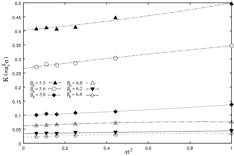
Figure 6: Extrapolation of the string tension to the Hamiltonian limit $\Delta\tau\rightarrow 0$. The curves are the quadratic fits in $\Delta\tau^{2}$.

To check the accuracy of our method, we compare our extrapolated estimates with Hamiltonian estimates obtained by using an exact linked cluster expansion (ELCE) Hamer86 . However, for such a comparison we must take into account the difference of scales between Euclidean and Hamiltonian regimes. The Hamiltonian coupling parameter $\lambda=6/g^{4}_{H}$, where $g_{H}=\lim_{\xi\rightarrow\infty}g_{\xi}$ may be related to $\beta_{E}$ through the relation Hasenfratz81

$$\beta_{E}=\sqrt{6\lambda}-0.07848.$$ (27)

We see that our results agree well with those obtained from ELCE although less accurate in the small $\beta_{E}$ region. We do not expect precise agreement in this region, since ELEC results correspond to the energy per unit length of a “string” of flux along one axis, whereas our estimates refer to the decay exponent of space-like Wilson loops. We do not show here the GFMC results Hamer00 , which were obtained from Creutz ratios on very small loops, and therefore subjected to large finite-size effects. Our results in the Hamiltonian limit for the string tension $K$, hadronic scale $r_{0}$ in terms of the lattice spacing $a_{s}$ and the Coulomb coupling $e_{c}$ are shown in Table 9. Also are shown, for comparison, the previous Hamiltonian estimates from ELCE.

Table 9: Results for the string tension $K$ and hadronic scale $r_{0}$ and the Coulomb coupling $e_{c}$ in the Hamiltonian limit.

$\lambda$	$K$	$e_{c}$	$a_{s}/r_{0}$	$K$ from ELCE Hamer86
4.2991	0.76(3)	0.393(4)	0.7790	0.664(6)
4.6437	0.67(2)	0.403(4)	0.7354	0.563(5)
5.0022	0.56(1)	0.367(3)	0.7120	0.404(3)
5.1865	0.395(9)	0.324(3)	0.5158	0.34(2)
5.3741	0.265(4)	0.220(1)	0.4311	0.24(4)
5.7594	0.096(3)	0.203(1)	0.2580	0.107(8)
6.1580	0.061(2)	0.245(2)	0.2090
6.5698	0.033(2)	0.262(2)	0.1542
6.9951	0.021(1)	0.251(2)	0.1219

To obtain estimates of glueball masses in the Hamiltonian limit, an extrapolation of the data points obtained at constant $\beta_{E}$ for various anisotropies ($\Delta\tau=1-0.25$) is performed in powers of $\Delta\tau^{2}$. Error estimates for the extrapolation may be obtained by the “linear, quadratic, cubic” extrapolation method Pradeep00 . Figure 7 shows our estimates for the scalar glueballs as a function of $\Delta\tau^{2}$ for various fixed $\beta_{E}$ values. Unlike the string tension, the scalar mass depends rather strongly on $\Delta\tau$. This can be seen from the slope and the curvature in the extrapolation to the Hamiltonian limit in the plot. This may be due to the presence of the $O(a_{t}^{2})$ errors in the standard Wilson action. In the large $\beta_{E}$ region we, however, see a smooth variation of the scalar mass with $\Delta\tau^{2}$.

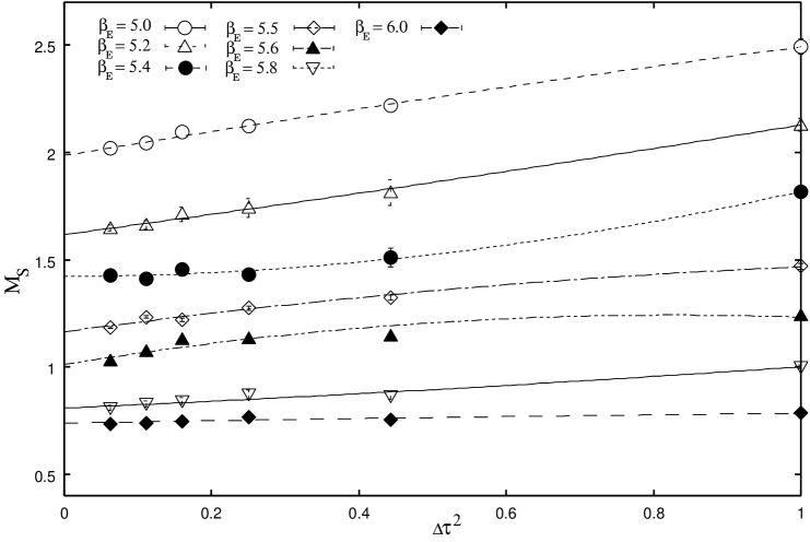
Figure 7: Extrapolation of the scalar glueball mass (in lattice units) to the Hamiltonian limit $\Delta\tau\rightarrow 0$, for fixed $\beta_{E}$. The lines show quadratic fits to the data in $\Delta\tau^{2}$.

The extrapolation of axial vector and tensor glueball masses to the Hamiltonian limit is shown in Figs. 8 and 9 respectively. This is performed again in powers of $\Delta\tau^{2}$, in a fashion similar to the scalar glueball. In both these channels we note that both show a strong dependence on $\Delta\tau$: in the intermediate $\beta_{E}$ region there is a factor of 2 - 3 difference between the values at $\Delta\tau=0$ and $\Delta\tau=1$. Since the leading discretization errors in the tensor glueball masses are expected to be $O(a_{t}^{2},a_{s}^{2},\alpha_{s}a_{s}^{2})$, this difference may be attributed to the presence of $O(a_{t}^{2})$ errors. However, in the extreme anisotropic region, the results differ very little; this is obvious since the expected $O(a_{t}^{2})$ errors decrease as aspect ratio $\xi=1/\Delta\tau$ is increased.

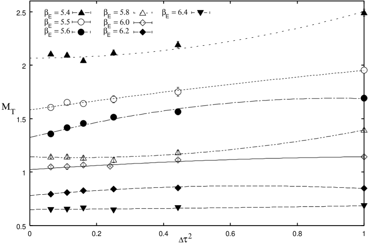
Figure 8: Extrapolation of the tensor glueball mass (in lattice units) to the Hamiltonian limit $\Delta\tau\rightarrow 0$, for fixed $\beta_{E}$. The lines show quadratic fits to the data in $\Delta\tau^{2}$.

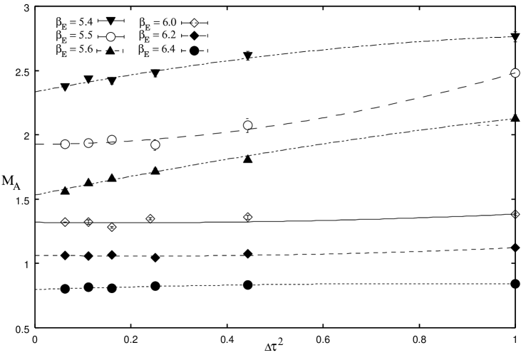
Figure 9: Extrapolation of the axial glueball mass (in lattice units) to the Hamiltonian limit $\Delta\tau\rightarrow 0$, for fixed $\beta_{E}$. The lines show quadratic fits to the data in $\Delta\tau^{2}$.

Our Hamiltonian estimates for the scalar $M_{S}(=a_{t}m_{0^{++}})$, axial vector $M_{A}(=a_{t}m_{1^{+-}})$ and tensor $M_{T}(=a_{t}m_{2^{++}})$ glueballs together with the Hamiltonian coupling $\lambda$, calculated from Eq. (27) are shown in Table 10.

Table 10: Glueball masses in the Hamiltonian limit.

$\lambda$	$M_{S}$	$M_{A}$	$M_{T}$
4.2991	1.98(1)
4.6437	1.61(1)
5.0022	1.42(1)	2.09(2)	2.33(2)
5.1865	1.16(2)	1.58(1)	1.80(1)
5.3741	1.01(2)	1.40(1)	1.79(1)
5.7594	0.84(1)	1.14(2)	1.41(2)
6.1580	0.738(9)	1.034(9)	1.32(1)
6.5698	0.58(1)	0.78(1)	1.06(1)
6.9951	0.47(1)	0.64(1)	0.79(1)

V.2 Asymptotic scaling

An interesting question concerns the onset of “scaling”, which is often interpreted to mean that the physical quantities should become independent of the coupling in the weak-coupling regime. Here, we examine more closely the asymptotic scaling, given by the two-loop perturbative $\beta$-function Osterwnlder78

$$am=C_{m}\mbox{exp}\bigg{(}-\frac{1}{2b_{0}g^{2}}\bigg{)}\big{(}b_{0}g^{2}\big{)}^{-b_{1}/2b_{0}^{2}}\left[1+O(g^{2})\right],$$ (28)

where

$$b_{0}=\frac{11}{16\pi^{2}},\hskip 14.22636ptb_{1}=\frac{102}{(16\pi^{2})^{2}},$$

with the aim to establish that results approach the expected scaling form in the weak-coupling regime. The coupling $g$ refers to the Hamiltonian coupling $g_{H}$ in this case. In general, the most accurately calculated physical quantity is the string tension $K$, and hence the dimensionless ratio $m/\sqrt{K}$, since the leading corrections to such a ratio are known to be of the order $O(1/\zeta)^{2}$ Teper98 , where $\zeta$ is some length scale. However, it is well known that behavior of the string tension is quite different over the range of coupling: it follows neither two-loop nor three-loop scaling at these couplings and there is no universal Callan-Symanzik functions that can accommodate both string tension and glueball mass down to this coupling range.

Fig. 10 shows the asymptotic scaling behavior of scalar glueball mass, $M_{S}$, as a function of $\sqrt{\lambda}$. The dotted-line is the Hamiltonian strong-coupling expansion to the order $\beta_{H}^{7}$ Hamer89 and the solid line represents a fit to the Hamiltonian weak-coupling asymptotic form (28). It can be seen that our estimates appear to match nicely onto the strong and weak coupling expansions in their respective limits. The strong coupling series is not well behaved as the approximants begin to diverge as the crossover region is reached, hence allowing only rough estimates. For comparison we also show the results obtained from plaquette expansion Hollenberg98 , which are found to converge quickly in the strong coupling region and diverge as the transition region is approached. The results are somewhat lower than our estimates, but are almost compatible within errors.

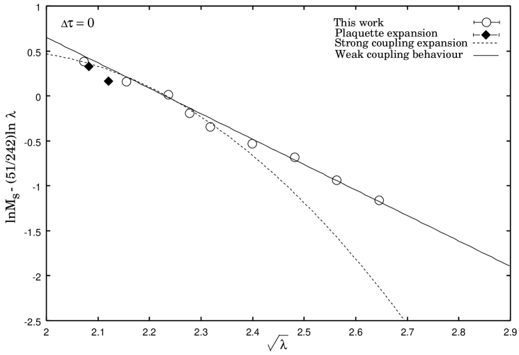
Figure 10: The asymptotic scaling behavior of scalar mass gap as a function of Hamiltonian coupling. The errors are smaller than the data points.

In the weak-coupling region, the scalar glueball mass appears to adhere accurately to the expected asymptotic scaling behavior. An unconstrained fit of the form (28) to the data in the range $2.3\leq\sqrt{\lambda}\leq 2.65$, which corresponds to $5.6\leq\beta_{E}\leq 6.4$, gives a scaling slope of $2.83\pm 0.17$ which is consistent, within errors, with the predicted value of 2.90. It is interesting to note that our estimate of $C_{m}=260\pm 10$ agrees well with the value found in plaquette expansion when the curves are matched onto the scaling form at $\sqrt{\lambda}=2.02$.

V.3 Extrapolation to the continuum limit

To extrapolate the results given in Table 10 to zero lattice spacing, we combine the glueball mass estimates with the determinations of the hadronic scale $r_{0}/a_{s}$. Fig. 11 shows the dimensionless product of $r_{0}$ and the scalar glueball mass estimates as a function of $(a_{s}/r_{0})^{2}$. Also are shown for comparison the earlier Hamiltonian estimates from the series expansion Hamer89 , t-expansion Lana91 and the plaquette expansion Hollenberg98 .

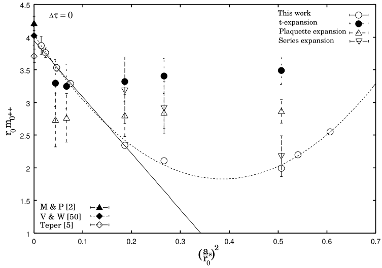
Figure 11: Scalar glueball mass estimates in terms of $r_{0}$ as a function of the lattice spacing $(a_{s}/r_{0})^{2}$. The solid and dashed lines represent linear and quadratic extrapolation of the data to the continuum limit. Results from different methods are also shown for comparison.

It can be seen from Fig. 11 that scalar glueball mass shows a peculiar feature. There is no clear sign of the dimensionless quantity $r_{0}m_{0^{++}}$ reaching to a constant value. As $a_{s}$ is increased from zero, the scalar mass first decreases, reaching a minimum near $a_{s}/r_{0}\approx 0.6$, the mass then gradually increases with $a_{s}$.

The origin of the “dip” in the scalar glueball mass is attributed to the sensitivity of this state to discretization errors in the standard Wilson gauge action. The dip is reduced by about half when classically improved action Norman98 is used and further reduced when the classical improvement is supplemented by tadpole improvement Morningstar97 ; Morningstar99 . This implies that the origin of the dip lies, at least in part, in discretization errors. If this picture is correct then one might expect the dip to be further reduced (or even eliminated ) if one accounts for the perturbative renormalization of action. This would remove the leading $O(\alpha_{s}a^{2})$ discretization errors in the tree-level, tadpole-improved action. However before making a definitive conclusion regarding the observed sensitivity, one needs to compute the full radiative corrections to the action. Such calculations are under investigation and we intend to report on these studies in future. The fact that the scalar glueball is less sensitive to the finite-volume effects (Fig. 5) than the tensor state and somewhat larger lattice spacing dependence in the scalar mass could indicate that scalar glueball is smaller in size.

To extract the results in the continuum limit we fit the mass measurements by the following three-parameter fitting function:

$$\varphi(a_{s})=r_{0}m_{G}+c_{1}(a_{s}/r_{0})^{2}+c_{2}(a_{s}/r_{0})^{4},$$ (29)

where $r_{0}m_{G}$, $c_{1}$ and $c_{2}$ are fit parameters. The function yields a continuum limit $r_{0}m_{0^{++}}=4.03\pm 0.05$ MeV. An extrapolation of the data, in the range $0.014\leq(a_{s}/r_{0})^{2}\leq 0.18$ (with $5.6\leq\beta_{E}\leq 6.4$), using a linear fit of the form

$$\varphi_{1}(a_{s})=r_{0}m_{G}+c_{0}(a_{s}/r_{0})^{2}$$ (30)

yields $r_{0}m_{0^{++}}=3.94\pm 0.02$.

A comparison with previous continuum limit estimates obtained by Morningstar and Peardon Morningstar99 using tadpole improved action, Vaccarino and Weingarten Vaccarino99 and Teper Teper98 using standard Wilson action on isotropic lattice shows that our result for the scalar mass is lower than that obtained by Morningstar and Peardon Morningstar99 but in good agreement with result obtained by Vaccarino and Weingarten Vaccarino99 and more accurate than the results obtained in Ref. Teper98 . We, however, do not expect a complete agreement with the results obtained in Ref. Morningstar99 which were computed for a different action. A comparison with the earlier Hamiltonian results shows that our present estimates are higher than those obtained previously. The $t$-expansion Lana91 results, obtained from 1/3 D-Pade approximants, reach a constant value near the continuum and are higher than the plaquette expansion estimates Hollenberg98 , obtained by taking the average of the curves for various values of set parameter. A continuum extrapolation of the $t$-expansion estimates leads to $r_{0}m_{0^{++}}=3.24\pm 0.025$ whereas the plaquette expansion estimates give $2.75\pm 0.018$. We observe that our result is an excellent improvement over all previous Hamiltonian results.

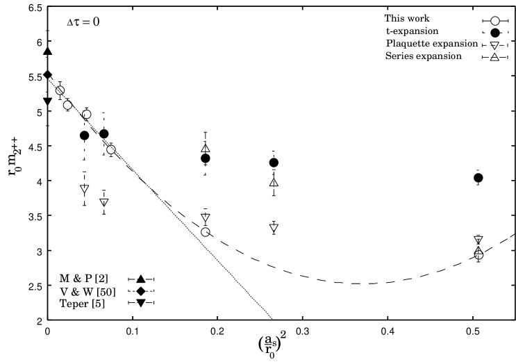
Figure 12: Same as Fig. figCona1pp but for the tensor glueball.

Figs. 12 and 13 show, respectively, the continuum limit extrapolation of the tensor and axial vector glueball masses in terms of $r_{0}$ against lattice spacing $(a_{s}/r_{0})^{2}$. Although the leading discretization errors in the tensor glueball mass are expected to be $O(a_{t}^{2},a_{s}^{2},\alpha_{s}a_{s}^{2})$, the tensor glueball data show less significant finite-spacing errors in contrast to the scalar mass. This could indicate that the tensor glueball has a larger size. For our final estimates of the tensor and axial vector glueball masses, we perform fits using Eq. (29) while constraining the fit parameters to be the same for both the fitting functions. The fits yields $r_{0}m(2^{++})=5.54\pm 0.06$ and $r_{0}m(1^{+-})=7.17\pm 0.17$ for the tensor and axial vector glueballs respectively. These results are in agreement with the estimates obtained in Ref. Vaccarino99 , however, lower than the results obtained in Ref. Morningstar99 . This is most probably due to the strong curvature in our extrapolations for the tensor and axial vector glueballs. In the large $a_{s}$ region our results for the tensor glueballs are in good agreement with plaquette expansion estimates and comparable within errors to the $t$-expansion results in the small $a_{s}$ region. Near the continuum our estimates are higher than previous Hamiltonian estimates. A linear fits to the $t$-expansion data yield continuum values $4.61\pm 0.08$ and $5.56\pm 0.11$ for $r_{0}m_{2^{++}}$ and $r_{0}m_{1{+-}}$ respectively.

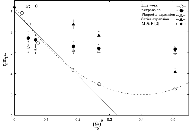
Figure 13: Same as Fig. figCona1pp but for the axial vector glueball mass.

The continuum extrapolation of the dimensionless mass ratio, $R_{T}=m_{2^{++}}/m_{0^{++}}$, which is expected to be more easily amenable, as a function of $(a_{s}/r_{0})^{2}$ is shown in Figs. 14. The mass ratio $R_{T}$ decreases slightly as we move from larger to smaller $a_{s}$ and appears to reach a level near the continuum, but within statistical errors, they can be fitted by a straight limit, giving $R_{T}=1.36\pm 0.01$ at $a_{s}\to 0$. In the continuum limit, our results agree well with the Hamiltonian results Hamer89 ; Lana91 ; Hollenberg98 . This is in excellent agreement with results from the previous studies on Euclidean lattices. Since the Hamiltonian formulation is thought of as a very asymmetric Euclidean theory, this agreement provides a test of universality between the two formulations. It is interesting to note that mass ratio $R_{T}$ in SU(2) QCD exhibits similar features as that in SU(3) theory: the SU(2) $R_{T}$ rises to a value of approximately 1.5 over the intermediate volume region Teper98 . Our estimates for the glueball masses and mass ratio are shown and compared with previous results from various other studies in Table 11.

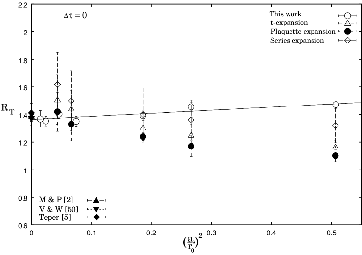
Figure 14: Extrapolation of the mass ratios to the continuum limit. The solid line is a linear fit to the data.

We see the evidence that the axial vector mass is definitely greater than the scalar and tensor masses for all couplings analyzed here. This is in accordance with the claim made by Hamer Hamer89 that corresponding mass ratios are strictly greater than one for all finite couplings.

Table 11: Glueball masses and the mass ratio in the continuum limit. The values indicated in bold are our final continuum mass estimates. The fitting function to the data is given in Eq. (29).

Reference	$r_{0}m_{0^{++}}$	$r_{0}m_{2^{++}}$	$r_{0}m_{1^{+-}}$	$R_{T}$
This work	4.03(5)	5.54(6)	7.2(2)	1.36(2)
M $\&$ P Morningstar99	4.21(11)	5.85(2)	7.18(4)	1.39(4)
V $\&$ W Vaccarino99	4.0(1)	5.5(2)		1.37(5)
Teper Teper98	3.65(11)	5.1(3)		1.41(7)
UKQCD Bali93	3.78(12)	5.53(24)	6.90(8)	1.44(6)
Hamiltonian Hamer89 ; Lana91	3.0 - 3.3	4.25 - 4.60	5.40 - 5.80	1.2-1.6

Finally, we convert our glueball mass estimates into physical units by assigning value to the hadronic scale. The estimate for $r_{0}$ was obtained by combining the results from various quenched lattice simulations with the standard Wilson action Morningstar97 . The simple average $r_{0}^{-1}=410\pm 20$ MeV of the determinations in Ref. Morningstar97 was taken as our estimate of the hadronic scale. For the lowest-lying scalar glueball we obtain $m(0^{++})=1654\pm 83\pm 70$ MeV. The tensor and axial vector masses, for which the extrapolation to zero lattice spacing encountered no problems, are $m(2^{++})=2272\pm 115\pm 125$ MeV and $m(1^{+-})=2940\pm 165\pm 120$ MeV, where the first error comes from uncertainty in $r_{0}m_{G}$ and second error comes from the uncertainty in $r_{0}^{-1}$. Our estimates are in good agreement with those found in Ref. Vaccarino99 but are under the predicted values for the resonances $f_{0}(1710)$, $f_{2}(2400)$ by about 10-15$\%$. However, for direct comparison with the experiment, we have to take into account the contribution from corrections due to the light quark effects and mixing with conventional hadrons: the quenched approximation will easily lead to an underestimate of the simulated values. A possible solution to this problem is to construct a QCD Hamiltonian that couples conventional hadrons and glueballs of identical $J^{PC}$ so that physical states are a linear combination of hadron and glueball states. This will shed some light on the contents and dominant components of the predicted resonances in the scalar and excited glueball states. The glueball with exotic quantum numbers will, however, not mix with the conventional hadrons and would be ideal for establishing the existence of glueballs.

VI CONCLUSIONS

In this work we used standard Euclidean MC methods to extract the Hamiltonian limit of 4-dimensional SU(3) LGT. By taking the renormalization of both the anisotropy and couplings we have calculated the string tension and glueball masses in the extreme anisotropic limit. We have found that the renormalization of the couplings and anisotropy has a large influence on extrapolating our results to the Hamiltonian limit $\Delta\tau\rightarrow 0$. It has been suggested that this renormalization has a much smaller effect for improved actions Morningstar97 ; Morningstar99 , however later calculations Sakai00 showed that the discrepancy between the couplings $\beta_{\xi}$ and $\beta_{E}$ reach a maximum near high anisotropies ($\Delta\tau\leq 0.333$). It would be interesting to see how this renormalization influences the extrapolation of the results for improved actions to the Hamiltonian limit.

Estimates for the scalar, tensor and axial vector glueballs were extrapolated to the continuum limit and the results are presented in terms of the hadronic scale $r_{0}^{-1}$. Extrapolation of the scalar glueball mass to the continuum limit was problematic than those of tensor and axial vector masses. In the continuum limit the mass ratio $R_{T}$ was observed to scale to $1.36\pm 0.2$. We have demonstrated that there is a broad agreement between our results and the results obtained in the Euclidean limit of the theory and a substantial improvement over previously known estimates calculated within the Hamiltonian formulation. This demonstrates clear evidence of the universality between the Euclidean and Hamiltonian formulations. Our main aim for examining anisotropic lattice was to investigate alternative MC procedures for obtaining reliable results in the Hamiltonian limit, in view of the lack of a reliable numerical method for Hamiltonian LGT. We have found that standard Euclidean MC approach is more successful than other quantum MC methods, in particular the Greens Function MC techniques.

From the accuracy of the results obtained here we conclude that standard MC approach is a preferred technique for calculating physical observables in the Hamiltonian limit, just as in the Euclidean formulation. In order to make the Euclidean MC method a more valuable tool in the Hamiltonian LGT, it will be crucial to show that it allows one to treat eventually matter fields in the non-Abelian case. The major disadvantage of this approach is the cost in computer time, as several configuration sets must be generated to obtain one data point.

- (1) C. J. Morningstar and M. J. Peardon, Phys. Rev. D 60, 034509 (1999); Nucl. Phys. B (Prog. Suppl.) 73, 927 (1999).
- (2) C. J. Morningstar and M. J. Peardon, Phys. Rev. D 56, 4043 (1997).
- (3) N. H. Shakespeare and H. D. Trottier, Phys. Rev. D 59, 014502 (1999).
- (4) M. Teper, Phys. Lett. B 397, 223 (1997) [arXiv:hep-lat/9701003].
- (5) R. Gupta et al., Phys. Rev. D 43, 2301 (1991).
- (6) A. Vaccarino and D. Weingarten, Phys. Rev. D 60, 114501 (1999).
- (7) C. Michael, G. Tickle and M. Teper, Phys. Lett. B 207, 313 (1988).
- (8) C. Michael, J. Phys. G 13, 1001 (1987).
- (9) UKQCD Collaboration, G. Bali et al., Phys. Lett. B 309, 378 (1993).
- (10) D. Weingarten, Nucl. Phys. B (Prog. Suppl.) 34, 29 (1993).
- (11) W. Lee and D. Weingarten, Nucl. Phys. B (Prog. Suppl.) 73, 249 (1999).
- (12) X.Q. Luo, and Q. Chen, Mod. Phys. Lett. A 11, 2435 (1996) [arXiv:hep-ph/9604395].
- (13) X.Q. Luo, Q. Chen, S. Guo, X. Fang, and J. Liu, Nucl. Phys. B (Proc. Suppl.)53, 243 (1997).
- (14) X. Q. Luo, S. H. Guo, H. Kroger and D. Schutte, Phys. Rev. D 59, 034503 (1999).
- (15) E. B. Gregory, S. H. Guo, H. Kröger and X. Q. Luo, Phys. Rev. D 62, 054508 (2000).
- (16) X. Q. Luo, E. B. Gregory, S. H. Guo and H. Kröger hep-ph/0011120.
- (17) Y. Fang and X. Q. Luo, Phys. Rev. D 69, 114501 (2004).
- (18) X. Q. Luo, Phys. Rev. D 70, 091504 (2004) (Rapid Commun.).
- (19) C. Hamer, Phys. Lett. B 224, 339 (1989).
- (20) D. Horn and M. Weinstein, Phys. Rev. D 30, 1256 (1984).
- (21) D. Horn and G. Lana, Phys. Rev. D 44, 2864 (1991).
- (22) L. Hollenberg, Phys. Rev. D 47, 1640 (1993).
- (23) M. Wilson and C. Hollenberg, Austral. J. Phys. 51, 35 (1998).
- (24) D. W. Heys and D. R. Stump, Phys. Rev. D 28, 2067 (1983).
- (25) D. W. Heys and D. R. Stump, Nucl. Phys. B 257, 19 (1985).
- (26) D.W. Heys and D.R. Stump, Phys. Rev. D 30, 2674 (1984).
- (27) S. A. Chin, C. Long and D. Robson, Phys. Rev. Lett. 57, 2779 (1986).
- (28) S. A. Chin, C. Long and D. Robson, Phys. Rev. D 37, 3001 (1988).
- (29) C. Long, D. Robson and S. A. Chin, Phys. Rev. D 37, 3006 (1988).
- (30) C. J. Hamer, M. Samaras and R. J. Bursill, Phys. Rev. D 62, 074506 (2000).
- (31) R. Blankenbecler and R.L. Sugar, Phys. Rev. D 27, 1304 (1983).
- (32) T. A. DeGrand and J. Potvin, Phys. Rev. D 31, 871 (1985).
- (33) C. R. Allton, C. M. Yung and C. J. Hamer, Phys. Rev. D 39, 3772 (1989).
- (34) C. J. Hamer, K. C. Wang and P. F. Price, Phys. Rev. D 50, 4693 (1994).
- (35) M. Loan, M. Brunner, C. Sloggett and C. Hamer, Phys. Rev. D 68, 034504 (2003).
- (36) M. Loan, T. Byrnes and C. Hamer, Eur. Phys. J. C 31, 397 (2003) [arXiv:hep-lat/0303011].
- (37) M. Loan and C. Hamer, Phys. Rev. D 70, 014504 (2004).
- (38) T. Byrnes el at, Phys. Rev. D 69, 074509 (2004).
- (39) T. R. Klassen, Nucl. Phys. B 533, 557 (1998) [arXiv:hep-lat/9803010].
- (40) R. F. Dashen and D. J. Gross, Phys. Rev. D 23, 2340 (1981).
- (41) A. Hasenfratz and P. Hasenfratz, Nucl. Phys. B 193, 210 (1981).
- (42) F. Karsch, Nucl. Phys. B 205, 285 (1982).
- (43) C. Hamer, Phys. Rev. D 50, 1657 (1995).
- (44) N. Cabibbo and E. Marinari, Phys. Lett. B 119, 387 (1982).
- (45) S. L. Adler, Phys. Rev. D 37, 458 (1988). M. Creutz, Phys. Rev. D 36, 515 (1987).
- (46) F. R. Brown and T. J. Woch, Phys. Rev. Lett. 58, 2394 (1987).
- (47) M. Albanese et al. [APE Collaboration], Phys. Lett. B 192, 163 (1987).
- (48) M. Falcioni, M. L. Paciello, G. Parisi and B. Taglienti, Nucl. Phys. B 251, 624 (1985).
- (49) M. Luscher, Commun. Math. Phys. 104, 177 (1986).
- (50) C. J. Hamer, A. C. Irving and T. E. Preece, Nucl. Phys. B 270, 553 (1986).
- (51) A. Hasenfratz, E. Hasenfratz and P. Hasenfratz, Nucl. Phys. B 180, 353 (1981).
- (52) M. Luscher, Nucl. Phys. B 180, 317 (1981).
- (53) P. Sriganesh, R. Bursill and C. J. Hamer, Phys. Rev. D 62, 034508 (2000).
- (54) K. Osterwalder and E. Seiler, Annals Phys. 110, 440 (1978).
- (55) Particle Data Group, Euro. Phys. J. C3, 1 (1998).
- (56) S. Sakai, T. Saito and A. Nakamura, Nucl. Phys. B 584, 528 (2000).