Excited Baryon Spectroscopy from Lattice QCD:
Finite Size Effect and Hyperfine Mass Splitting

Abstract

A study of the finite-size effect is carried out for spectra of both ground-state and excited-state baryons in quenched lattice QCD using Wilson fermions. Our simulations are performed at $\beta=6/g^{2}=6.2$ with three different spatial sizes, $La\sim$ 1.6, 2.2 and 3.2 fm. It is found that the physical lattice size larger than 3 fm is required for $\Delta$ states in all spin-parity ($J^{P}=1/2^{\pm},3/2^{\pm}$) channels and also negative-parity nucleon ($N^{*}$) state ($J^{P}=1/2^{-}$) even in the rather heavy quark mass region ($M_{\pi}\sim 1.0$ GeV). We also find a peculiar behavior of the finite-size effect on the hyperfine mass splittings between the nucleon and the $\Delta$ in both parity channels.

I Introduction

In the past several years, many lattice studies on excited baryon spectroscopy have been made within the quenched approximation after the pioneering attempts NstarPioneers . Although these calculations gave results of negative-parity baryon masses in gross agreement with experiments Sasaki:2001nf ; Gockeler:2001db ; Melnitchouk:2002eg ; Zanotti:2003fx ; Mathur:2003zf ; Nemoto:2003ft ; Brommel:2003jm ; Burch:2004he ; Guadagnoli:2004wm , the higher precision study requires accurate controls of systematic errors, which may arise from the quenched approximation, chiral extrapolation, nonzero lattice spacing and finite-size effect. The first and second errors might appear most seriously in spectra of the excited states and should be entangled with each other due to possible decay processes. This complicated issue, however, ought to be postponed since the current dynamical simulations are still limited even for the ground-state baryons. It is worth emphasizing that the quenched lattice QCD is still useful to investigate several long standing puzzles in excited baryon spectroscopy, such as the level ordering problem between the negative-parity nucleon $N^{*}(1535)$ and the Roper resonance $N^{\prime}(1440)$, the structure of the $\Lambda(1405)$ and so on Leinweber:2004it .

Instead of using small lattice spacing, many calculations have adopted sophisticated lattice discretization schemes for fermions, the improved fermion actions Gockeler:2001db ; Melnitchouk:2002eg ; Zanotti:2003fx ; Nemoto:2003ft or chiral fermions Sasaki:2001nf ; Mathur:2003zf ; Brommel:2003jm ; Burch:2004he , in excited baryon spectroscopy to reduce the cutoff effect and improve the chiral behavior. However, there is not so much attention paid to the finite-size effect. Indeed, most of all simulations are performed with spatial lattice sizes $La\sim 1.6-2.2$ fm. This is because the finite-size study has been hardly done due to large computational costs. In this study, we utilize the standard Wilson fermion action, the computational requirements of which are relatively cheap. Therefore, we systematically perform the finite-size study for excited baryon spectroscopy.

For the finite-size effect, after the pioneering analytic consideration Luscher:1985dn , where the finite-size behavior of hadron masses obeys the exponential form $M_{\infty}-M_{L}\simeq L^{-1}\exp(-L/L_{0})$, it has been found that this behavior is rather described by a power law $\simeq L^{-n}$ with $n=2-3$ Fukugita:1992jj . This power-law behavior can be interpreted by the “wave function” squeezed on a finite lattice from the phenomenological point of view. The dependence of the finite-size effect on the spatial boundary condition which is found earlier Gupta:1982hu ; Martinelli:1982bm , can also be explained by this interpretation Aoki:1993gi . Ref. Aoki:1993gi reported that the lattice size $La>2.5$ fm is required for the nucleon ground-state ($N$) in quenched lattice QCD.

In the non-relativistic quark model with a harmonics-oscillator potential $H=\frac{1}{2m}\hat{p}^{2}+\frac{1}{2}m\omega^{2}\hat{r}^{2}$, the energy level and the root mean square radius can be estimated as $E_{N}=\hbar\omega(N+\frac{3}{2})$ and $r_{\rm rms}=\sqrt{\frac{\hbar}{m\omega}(N+\frac{3}{2})}$, respectively. The negative-parity nucleon ($N^{*}$) is identified as $N=1$ state, which corresponds to the first orbital excitation. It turns out that a ratio of the root mean square radii between the $N^{*}$ and the $N$ states is estimated as $r_{\rm rms}^{N^{*}}/r_{\rm rms}^{N}=\sqrt{5/3}\sim 1.3$. This means that the finite-size effect stemming from the hadron size squeezed is expected to become much serious for the excited-state baryons rather than the ground-state baryon. According to a crude estimate with this simple model, the lattice size $La>2.5\times 1.3\sim 3.2$ fm might be required for the excited baryon spectroscopy.

The organization of our paper is as follows. In Sec.II, we first review the basic idea of the parity projection in lattice simulations. In recent years, the parity projection technique is greatly appreciated in determining the parity of the pentaquark state in lattice QCD Sasaki:2004vz ; Sasaki:2003gi . Unfortunately, however, there are some initial confusions about the parity assignment Sasaki:2004vz . Thus, we describe details of the precise parity projection, which is always adopted by one of authors in excited baryon spectroscopy Sasaki:2001nf ; Sasaki:2003gi ; Sasaki:2003xc . For the spectroscopy of the spin-3/2 state, i.e. the $\Delta$ baryon, appropriate spin projections are also described. Sec. III gives details of our Monte Carlo simulations and results of the finite-size study for various baryon states, such as the nucleon states in both parity channel ($J^{P}=1/2^{\pm}$) and the $\Delta$ states in all spin-parity channels ($J^{P}=1/2^{\pm},3/2^{\pm}$). Then, we discuss about mass splittings between hyperfine partners in both parity channels. Finally, in Sec. IV we summarize the present work.

II General Analytic Framework

II.1 Parity projection

In general, the local baryon operator should couple to both parity states. The local baryon operator is defined by the trilinear composite operator, which is composed of a local diquark operator and a spectator-like quark field Ioffe:1981kw as

$${\cal O}_{B}(x)=\varepsilon_{abc}\left(q_{a,i}^{T}(x)C\Gamma q_{b,j}(x)\right)\Gamma^{\prime}q_{c,k}(x)$$ (1)

where $\Gamma$ and $\Gamma^{\prime}$ stand for possible 16 Dirac matrices and $C$ is the charge conjugation matrix. The superscript $T$ denotes transpose. Indices $abc$ and $ijk$ have meanings as color and flavor respectively. The intrinsic parity of this operator is defined by the parity transformation of internal quark fields ${\cal P}q({\vec{x}},t){\cal P}^{{\dagger}}=+\gamma_{4}q(-{\vec{x}},t)$ as

$${\cal P}{\cal O}_{B}^{(\eta)}({\vec{x}},t){\cal P}^{{\dagger}}=\eta\gamma_{4}{\cal O}_{B}^{(\eta)}(-{\vec{x}},t),$$ (2)

where $\eta$ denotes the intrinsic parity of ${\cal O}_{B}^{(\eta)}$. However, due to the simple relation between the positive- and negative-parity operators: ${\cal O}_{B}^{(+)}(x)=\gamma_{5}{\cal O}_{B}^{(-)}(x)$ for the local baryon operator, the resulting two-point correlation functions are also related with each other Sasaki:2001nf as

$$\langle 0|{\cal O}^{(+)}_{B}(x)\overline{\cal O}_{B}^{(+)}(y)|0\rangle=-\gamma_{5}\langle 0|{\cal O}^{(-)}_{B}(x)\overline{\cal O}_{B}^{(-)}(y)|0\rangle\gamma_{5}\;.$$ (3)

This means that the two-point correlation function constructed from the local baryon operator has overlap with both parity states. Next, we consider the spin-1/2 baryon case as a typical example for the precise parity projection. The zero-momentum two-point function is given by the sum over all spatial coordinates ${\vec{x}}$,

$$G^{(\eta)}_{B}(t)=\sum_{\vec{x}}\langle 0|T\{{\cal O}^{(\eta)}_{B}({\vec{x}},t)\overline{\cal O}_{B}^{(\eta)}({\vec{0}},0)\}|0\rangle\;.$$ (4)

This two-point correlation has the asymptotic form Fucito:1982ip

$$G^{(\eta)}_{B}(t)=\frac{A_{\eta}}{2}\left(1+{\rm sgn}(t)\gamma_{4}\right)e^{-M_{\eta}|t|}-\frac{A_{-\eta}}{2}\left(1-{\rm sgn}(t)\gamma_{4}\right)e^{-M_{-\eta}|t|}$$ (5)

at large Euclidean time $t$. Here $M_{\eta}$ and $M_{-\eta}$ denote masses of the lowest-lying state in each parity channel. The amplitude $A_{\eta}$ ($A_{-\eta}$) is defined as $\langle 0|{\cal O}_{B}^{(\eta)}|B,\eta\rangle=\sqrt{A_{\eta}}u^{(\eta)}_{B}$. Here, it is worth noting that anti-particle contribution of the opposite parity state is propagating forward in time. Thus, the $+/-$ parity eigenstates in the forward propagating contribution can be obtained by choosing the appropriate projection $P^{(\eta)}_{\pm}=(1\pm\eta\gamma_{4})/2$, which is given in reference to the intrinsic parity of the utilized operator, $\eta$. This procedure is accomplished by taking the trace of the correlator over spinor with the relevant projection operator as $\frac{1}{4}{\rm Tr}\{P^{(\eta)}_{\pm}G_{B}^{(\eta)}(t)\}$ where the factor of 1/4 is our choice of normalization.

The lattice simulation is, however, performed on a lattice with finite extent $T$ in the time direction and (anti-)periodic boundary conditions. The definition of the forward propagating contribution is slightly ambiguous since the backward propagating can wrap the whole time range around the time boundary. Hereafter, for a simplicity, we take $\eta=+$. Under the (anti-)periodic conditions, the resulting correlation functions may be given by

$$G^{\rm p.b.c.}_{B}(t) = \sum_{n=-\infty}^{\infty}G_{B}(t+nT),$$ (6)

$$G^{\rm a.p.b.c.}_{B}(t) = \sum_{n=-\infty}^{\infty}(-)^{n}G_{B}(t+nT),$$ (7)

which certainly satisfy $G^{\rm p.b.c.}_{B}(t)=G^{\rm p.b.c.}_{B}(t+T)$ and $G^{\rm a.p.b.c.}_{B}(t)=-G^{\rm p.b.c.}_{B}(t+T)$ respectively.

For the region $0\leq t<T$, those correlation functions are expressed in the following forms:

$$G^{\rm p.b.c.}_{B}(t) = \sum_{n=0}^{\infty}A_{+}e^{-nM_{+}T}\left[\frac{1+\gamma_{4}}{2}e^{-M_{+}t}+\frac{1-\gamma_{4}}{2}e^{-M_{+}(T-t)}\right]$$ (8)

$$-\sum_{n=0}^{\infty}A_{-}e^{-nM_{-}T}\left[\frac{1-\gamma_{4}}{2}e^{-M_{-}t}+\frac{1+\gamma_{4}}{2}e^{-M_{-}(T-t)}\right],$$

$$G^{\rm a.p.b.c.}_{B}(t) = \sum_{n=0}^{\infty}A_{+}e^{-nM_{+}T}\left[\frac{1+\gamma_{4}}{2}e^{-M_{+}t}-\frac{1-\gamma_{4}}{2}e^{-M_{+}(T-t)}\right]$$ (9)

$$-\sum_{n=0}^{\infty}A_{-}e^{-nM_{-}T}\left[\frac{1-\gamma_{4}}{2}e^{-M_{-}t}-\frac{1+\gamma_{4}}{2}e^{-M_{-}(T-t)}\right]\;.$$

For details of above calculation, see Appendix A. In the large $T$ limit ($M_{+}T\gg 1$ and $M_{-}T\gg 1$), all $n\neq 0$ terms are negligible in a summation with respect to $n$, because of the factor $e^{-nM_{\pm}T}$. Thus, it turns out to be the form

$$G^{\rm p.b.c./a.p.b.c.}_{B}(t) \approx A_{+}\left[\frac{1+\gamma_{4}}{2}e^{-M_{+}t}\pm\frac{1-\gamma_{4}}{2}e^{-M_{+}(T-t)}\right]$$ (10)

$$-A_{-}\left[\frac{1-\gamma_{4}}{2}e^{-M_{-}t}\pm\frac{1+\gamma_{4}}{2}e^{-M_{-}(T-t)}\right]\;,$$

which has only a contribution from the first wrap-round effect. Clearly, even after the “parity projection” as $\frac{1}{4}{\rm Tr}\{P_{\pm}G_{B}^{\rm p.b.c./a.p.b.c.}(t)\}$, there remain unwanted contaminations from the backward propagating contributions due to the first wrap-round effect. However, one can easily find that the linear combination of two correlation functions with periodic and anti-periodic boundary conditions may prevent the first wrap-round effect:

$$\overline{G}_{B}(t)=\frac{1}{2}\{G_{B}^{\rm p.b.c.}(t)+G_{B}^{\rm a.p.b.c.}(t)\}\approx\left(\frac{1+\gamma_{4}}{2}\right)A_{+}e^{-M_{+}t}-\left(\frac{1-\gamma_{4}}{2}\right)A_{-}e^{-M_{-}t}.$$ (11)

Therefore, the parity projection are really accomplished through the operation $\frac{1}{4}{\rm Tr}\{P_{\pm}\overline{G}_{B}(t)\}$.

To achieve this in an efficient manner, we adopt a linear combination of the quark propagators with periodic and anti-periodic boundary conditions to construct the baryon two-point correlation function Sasaki:2001nf . The linear combination in the quark level automatically realizes the linear combination in the hadronic level, as shown below. First, the baryon two-point correlation function $G_{B}(t)$ can be schematically written by

$$G_{B}(t)=\sum_{\vec{x}}{\rm tr}_{c}\{S(x,0)\cdot S(x,0)\cdot S(x,0)\}$$ (12)

with the quark propagator $S(x,0)$ where $x=({\vec{x}},t)$ and $0=({\vec{0}},0)$. ${\rm tr}_{c}$ denotes a trace over color indices. We define the averaged quark propagator

$$\overline{S}(x,0)=\frac{1}{2}\left(S_{\rm P}(x,0)+S_{\rm AP}(x,0)\right),$$ (13)

where $S_{\rm P}(x,0)$ and $S_{\rm AP}(x,0)$ are subject to the periodic and anti-periodic boundary conditions in the time direction such as $S_{\rm P}({\vec{x}},t;0)=S_{\rm P}({\vec{x}},t+T;0)$ and $S_{\rm AP}({\vec{x}},t;0)=-S_{\rm AP}({\vec{x}},t+T;0)$. By inserting this linear combination into Eq.(12), the baryon two-point function is written as

$$G_{B}(t) = \frac{1}{8}\sum_{\vec{x}}{\rm tr}_{c}\left\{\left(S_{\rm P}(x,0)+S_{\rm AP}(x,0)\right)\cdot\left(S_{\rm P}(x,0)+S_{\rm AP}(x,0)\right)\cdot\left(S_{\rm P}(x,0)+S_{\rm AP}(x,0)\right)\right\}$$ (14)

$$= \frac{1}{2}\left\{G_{B}^{\rm p.b.c.}(t)+G_{B}^{\rm a.p.b.c.}(t)\right\},$$

where

$$G_{B}^{\rm p.b.c.}(t) = \frac{1}{4}\sum_{\vec{x}}{\rm tr}_{c}\left\{S_{\rm P}(x,0)\cdot S_{\rm P}(x,0)\cdot S_{\rm P}(x,0)+S_{\rm P}(x,0)\cdot S_{\rm AP}(x,0)\cdot S_{\rm AP}(x,0)\right.$$ (15)

$$\left.+S_{\rm AP}(x,0)\cdot S_{\rm P}(x,0)\cdot S_{\rm AP}(x,0)+S_{\rm AP}(x,0)\cdot S_{\rm AP}(x,0)\cdot S_{\rm P}(x,0)\right\}$$

and

$$G_{B}^{\rm a.p.b.c.}(t) = \frac{1}{4}\sum_{\vec{x}}{\rm tr}_{c}\left\{S_{\rm AP}(x,0)\cdot S_{\rm P}(x,0)\cdot S_{\rm P}(x,0)+S_{\rm P}(x,0)\cdot S_{\rm AP}(x,0)\cdot S_{\rm P}(x,0)\right.$$ (16)

$$\left.+S_{\rm P}(x,0)\cdot S_{\rm P}(x,0)\cdot S_{\rm AP}(x,0)+S_{\rm AP}(x,0)\cdot S_{\rm AP}(x,0)\cdot S_{\rm AP}(x,0)\right\}.$$

$G_{B}^{\rm p.b.c.}(t)$ has even numbers of $S_{\rm AP}(x,0)$ and then are satisfied with $G_{B}^{\rm p.b.c.}(t)=G_{B}^{\rm p.b.c.}(t+T)$. On the other hand, $G_{B}^{\rm a.p.b.c.}(t)$ includes odd numbers of $S_{\rm AP}(x,0)$ and is totally subject to the anti-periodic boundary condition, $G_{B}^{\rm a.p.b.c.}(t)=-G_{B}^{\rm a.p.b.c.}(t+T)$. We confirm that a linear combination of the quark propagators with periodic and anti-periodic boundary conditions makes a cancellation for the primal reflection from the time boundary in the baryon two-point function. This is also true for the meson two-point function as same as the baryon case.

II.2 Spin projection

In this subsection, we describe the spin projection, which is essential to deal with spin-3/2 baryon, namely the $\Delta$ state. We choose a interpolating operator for the $\Delta$, more specifically $\Delta^{++}$, as a simple trilinear composite operator:

$${\cal O}_{\mu}^{\Delta}(x)=\epsilon_{abc}\left(u_{a}^{T}(x)C\gamma_{\mu}u_{b}(x)\right)u_{c}(x),$$ (17)

where $u(x)$ represents the up quark field. This operator has the structure of the Rarita-Schwinger spinor (“vector-spinor”) so that the two-point function constructed from this operator can couple to both spin-3/2 and spin-1/2 states Leinweber:1992hy . We consider the two-point function at zero spatial momentum, which is given by

$$G_{\mu\nu}^{\Delta}(t)=\sum_{\vec{x}}\langle 0|T\{{\cal O}_{\mu}^{\Delta}({\vec{x}},t)\overline{\cal O}_{\nu}^{\Delta}({\vec{0}},0)\}|0\rangle.$$ (18)

Note that above $\Delta$ correlator can couple to the spin-3/2 state only if neither of $\mu,\nu$ are temporal indices. For the spatial Lorentz indices, $i,j=1,2,3$, Eq. (18) is expressed by the orthogonal sum of spin-3/2 and spin-1/2 components:

$$G^{\Delta}_{ij}(t)=\left(\delta_{ij}-\frac{1}{3}\gamma_{i}\gamma_{j}\right)G^{\Delta}_{3/2}(t)+\frac{1}{3}\gamma_{i}\gamma_{j}G^{\Delta}_{1/2}(t),$$ (19)

with appropriate spin projection operators Benmerrouche:1989uc . Respective spin parts, $G^{\Delta}_{3/2}(t)$ and $G^{\Delta}_{1/2}(t)$, possess both positive- and negative-parity contributions as same as Eq.(5). Some of excited $\Delta$ states such as the spin-1/2 $\Delta$ states can be accessed by the correlator $G^{\Delta}_{1/2}(t)$. These spin projected correlators are given by

$$G^{\Delta}_{3/2}(t) = \frac{3}{2}G^{\Delta}_{ii}(t)-\frac{1}{2}\sum_{k}\gamma_{i}\gamma_{k}G^{\Delta}_{ki}(t),$$ (20)

$$G^{\Delta}_{1/2}(t) = \sum_{k}\gamma_{i}\gamma_{k}G^{\Delta}_{ki}(t),$$ (21)

where an index $k$ should be summed over all spatial directions, but any specific choice is available for an index $i$. In this paper, we calculate all three direction for the spatial index $i$ and take an average of them to get the possible reduction of statistical errors.

According to the previous subsection, we perform the appropriate parity projection to apply to $G^{\Delta}_{3/2}(t)$ and $G^{\Delta}_{1/2}(t)$ as well. Then, we finally access to the four different spin-parity states of the $\Delta$ baryon, which correspond to the spin-3/2 positive-parity state ($\Delta_{3/2}$), the spin-3/2 negative-parity state ($\Delta^{*}_{3/2}$), the spin-1/2 positive-parity state ($\Delta_{1/2}$) and the spin-1/2 negative-parity state ($\Delta^{*}_{1/2}$). Of course, the $\Delta_{3/2}$ is the ground state of the $\Delta$ baryon. All others are the excited $\Delta$ baryons.

III Numerical Results

We generate ensembles of the quenched QCD configurations with the standard single-plaquette action at $\beta=6/g^{2}=6.2$ with three different lattice sizes, $L^{3}\times T=24^{3}\times 48$, $32^{3}\times 48$ and $48^{3}\times 48$, and compute the quark propagators by using Wilson fermion action at several values of the hopping parameter $\kappa$, which cover the range $M_{\pi}\approx 0.6-1.2$ GeV. Details of simulations are summarized in Tables 1 and 2.

For the update algorithm, we utilize the Metropolis algorithm with 20 hits at each link update. The first 10000 sweeps are discarded for thermalization. The ${\cal O}$(200-300) gauge ensembles in each simulation are separated by 1200 ($L$=48), 800 ($L$=32) and 600 ($L$=24) sweeps. For the matrix inversion, we use BiCGStab algorithm Frommer:1994vn and adopt the convergence condition $|r|<10^{-8}$ for the residues. We calculate a simple point-point quark propagator with a source location at $t_{\rm src}=6$. To perform the precise parity projection, we adopt a procedure to take an average of two quark propagators which are subject to periodic and anti-periodic boundary conditions in time, as described in Sec. II. We use the conventional interpolating operators, $\varepsilon_{abc}(u^{T}_{a}C\gamma_{5}d_{b})u_{c}$ for the nucleon and $\varepsilon_{abc}(u^{T}_{a}C\gamma_{\mu}u_{b})u_{c}$ for the $\Delta$ respectively.

All calculations were done on a Hitachi SR8000 parallel computer at KEK - High Energy Accelerator Research Organization, using the extended code based on the Lattice Tool Kit (LTK) Choe:2002pu . In this paper, we analyze the baryon-mass spectra in either parity channels with the conventional single exponential fit.

III.1 Spatial lattice-size dependence

We first discuss the finite-size effect on masses of all measured baryons. It is important to investigate how large size of physical lattice is required to neglect the finite-size effect on exited baryon spectroscopy. For this purpose, we perform numerical simulations at three different lattice sizes, $L^{3}\times T=24^{3}\times 48$, $32^{3}\times 48$ and $48^{3}\times 48$ for $\kappa=0.1506$ and 0.1497. Quenched $\beta=6.2$ corresponds to a lattice cutoff of $a^{-1}=2.913$ GeV, which is set by the Sommer scale Guagnelli:1998ud . Thus, the spatial extents in our study correspond to $La\simeq 1.6,~{}2.2$ and 3.2 fm in the physical unit. We will calculate the finite-size corrections to the baryon mass on each finite volume by comparison with values evaluated in the infinite volume limit.

We utilize the phenomenological powe- law formula to take the infinite volume limit for the observed masses as

$$aM_{L}=aM_{\infty}+cL^{-n}.$$ (22)

This power-law behavior can be interpreted by the hadron “wave function” squeezed on a finite lattice from the phenomenological point of view Fukugita:1992jj . As for the quenched simulation, Ref.Aoki:1993gi reported that the range of $n=1-2$ is preferable for the ground state of the nucleon. In this paper, we use the three different powers, $n=1,2$ and 3, and then determine which power-law behavior is most favorable for fitting data.

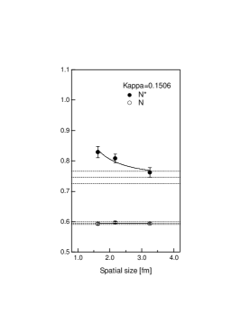
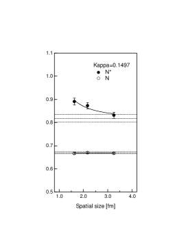
Figure 1: Masses of nucleons ($J^{P}=1/2^{\pm}$) in lattice unit as functions of spatial lattice size in the physical unit for $\kappa=0.1506$ (left figure) and $\kappa=0.1497$ (right figure). Solid curves are fits of the form $aM_{L}=aM_{\infty}+cL^{-n}$ with the value $n=2$. Horizontal dashed lines represent extrapolated values for each parity state in the infinite volume limit, together with their one standard deviation.

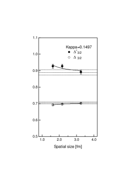
Figure 2: Masses of spin-3/2 $\Delta$ baryons in lattice unit as functions of spatial lattice size in the physical unit for $\kappa=0.1506$ (left figure) and $\kappa=0.1497$ (right figure). Solid curves and dashed lines are defined as in Figure 1.

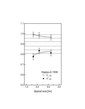
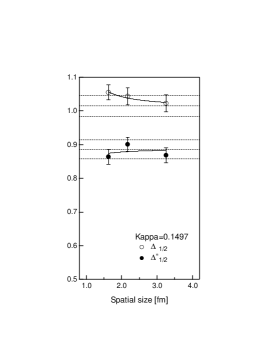
Figure 3: Masses of spin-1/2 $\Delta$ baryons in lattice unit as functions of spatial lattice size in the physical unit for $\kappa=0.1506$ (left figure) and $\kappa=0.1497$ (right figure). Solid curves and dashed lines are defined as in Figure 1.

In Figs.1-3 the lattice-size dependence of each baryon mass ($N$, $N^{*}$, $\Delta_{3/2}$, $\Delta^{*}_{3/2}$, $\Delta_{1/2}$, $\Delta^{*}_{1/2}$) is shown for two hopping parameters ($\kappa=0.1497$ and 0.1506), which correspond to the relatively heavier quark masses. All data included in Figs. 1-3 are summarized in Table 3. The quoted errors in figures represent only the statistical errors, which are obtained by a single elimination jack-knife method. Horizontal dashed lines represent the values in the infinite volume limit, which are evaluated in the case of $n=2$, together with their one standard deviation. A summary of masses in the infinite volume limit, which are guided by various power-law behaviors, is given in Table 4. In the case of the $N^{*}$ state, which receives the largest finite-size effect, the power two ($n=2$) is most preferable because of $\chi^{2}/N_{DF}\sim 1$.

For the nucleon case, we confirm that the finite-size effect is very small in the relatively heavier quark mass region. As shown in Fig. 1, all the data are located within $1\sigma$ of the value in the infinite volume limit at $\kappa=$0.1497 and 0.1506. We do not see any serious finite-size effect on the mass of the ground-state nucleon even at the smallest lattice size $La\simeq 1.6$ fm. In the mass of the negative-parity nucleon, a serious finite-size effect is not seen in the range of the spatial lattice size from 1.6 fm to 2.2 fm. This feature is consistent with that reported in Ref. Gockeler:2001db , in spite of the fact that their observed tendency of the size effect is opposite. Remarked that almost all subsequent lattice calculations to study the negative-parity nucleon are performed at the lattice size less than 2.2 fm. However, we find that the mass of the negative-parity nucleon suffers from the large finite-size effect in the range of the spatial lattice size from 2.2 fm to 3.2 fm. This means that the finite-size effect on the mass of the negative-parity baryon is unexpectedly severe and the spatial size is required at least 3 fm to remove this effect. What is the origin of the finite-size effect on the mass spectrum? In the phenomenological point of view, the “wave function” of baryon should be squeezed due to the small volume Fukugita:1992jj . The kinetic energy of internal quarks inside baryon is supposed to increase and thus the total energy of the three-quark system, which corresponds to the mass of baryon, should be pushed up. Such effect is expected to become serious for the excited state rather than the ground state. This intuitive picture seems to account for the observed trend of decreasing mass as the lattice size increases.

In the spin-3/2 $\Delta$ channel, however, we find that the finite-size effect has a different pattern: the ground-state mass of the spin-3/2 $\Delta$ becomes large as the lattice size increases. This behavior may originate from a hyperfine interaction. This possibility will be discussed later. On the other hand, the negative-parity state of the spin-3/2 $\Delta$, namely the $\Delta_{3/2}^{*}$, has the same pattern of the finite-size effect observed in the $N^{*}$ spectrum, while the finite-size correction of the $\Delta_{3/2}^{*}$ is relatively smaller than that of the $N^{*}$. As for the spin-1/2 $\Delta$ channel, all data at different lattice sizes are roughly consistent with each other within relatively large errors. However, the significant finite-size effect may be hidden behind the large statistical errors.

The finite-size effects on the masses of each baryon are summarized in Table 5. It is noteworthy that the finite-size corrections of $\Delta$ states ($J^{P}=3/2^{\pm}$) and negative-parity nucleon $N^{*}$ at spatial size $La$=1.6 fm can be seen even in the heavy quark region where that of the nucleon is almost negligible. Moreover, as we can learn from Figs.1-3, the spatial lattice size is required to be as large as 3 fm to remove the finite-size effect. The systematic error stemming from the finite-size effect at spatial size $La\simeq 3.2$ fm, $|(m_{\mathrm{3.2\hskip 2.0ptfm}}-m_{\infty})/m_{\infty}|$, is smaller than 2% for all measured states. Therefore, in the later discussion, we analyze data obtained on the largest lattice size of $48^{3}\times 48$ for spectroscopy of all hadrons.

Finally, we would like to comment on other possible formula such as the exponential form:

$$aM_{L}=aM_{\infty}+cL^{-1}\exp(-L/L_{0}),$$ (23)

which is inspired by the Lüscher’s formula for the asymptotic finite-size dependence of stable particle masses Luscher:1985dn . Here $1/L_{0}\sim M_{\pi}$ can be expected in the phenomenological sense. The full three-parameter fits tend to yield considerably low values of $1/L_{0}$. The obtained values are as low as $10^{-4}$ in lattice units. It is clearly inconsistent with a relation $1/L_{0}\sim M_{\pi}$ since our simulations are performed in the range of $M_{\pi}\sim 0.2-0.5$ in lattice units. If the parameter $L_{0}$ is fixed by $1/L_{0}=M_{\pi}$, the resulting $\chi^{2}/N_{DF}$ from the two-parameter fits is no longer reasonable. Therefore, the finite-size behavior that we observed here can be described by a power-law formula (22) rather than above exponential formula.

III.2 Chiral extrapolation

All data of hadron masses computed on lattice with spatial size $La\simeq 3.2$ fm are tabulated in Tables 6 and 7. We perform a covariant single exponential fit to two-point functions of each hadron in respective fitting ranges. All fits have a confidence level larger than 0.15 and $\chi^{2}/N_{DF}<1.5$. Our adopted ranges for fitting are basically determined by plateaus of each effective mass.

Next, we extrapolate masses of all calculated hadrons to the chiral limit using two types of fitting formula:

$$aM_{H}=c_{0}+c_{2}(aM_{\pi})^{2}$$ (24)

or

$$(aM_{H})^{2}=d_{0}+d_{2}(aM_{\pi})^{2},$$ (25)

where $c_{0}$, $c_{2}$, $d_{0}$, $d_{2}$ are numerical constants. We evaluate the systematic error by the difference between the chiral limit values obtained by two different fitting formulae. Hereafter, Eq. (24) and (25) are referred as the “linear” fit and the “curve” fit, respectively. The chiral limit values and their values of fitting $\chi^{2}$ are listed in Table 8. For the $\rho$ meson, the nucleon and the $\Delta_{3/2}$, in accordance with resulting $\chi^{2}$ values, we can determine that the curve fit is much preferable. However, for the other baryons, either fits yield acceptable values of $\chi^{2}$ because of the relatively large statistical errors on fitted data. However, the systematic error stemming from the difference of two fitting results is less than 10%. We then adopt the curve fit for all hadrons as the final analysis of chiral extrapolation.

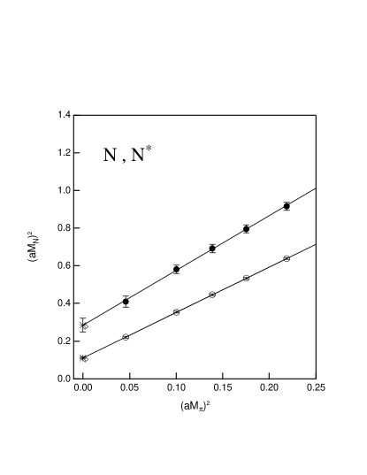
Figure 4: Squared masses of nucleons ($J^{P}=1/2^{\pm}$) in lattice unit as functions of squared pion mass. Circle symbols correspond to the negative-parity state (solid circles) and the positive-parity state (open circles). The extrapolated points in the chiral limit are represented by stars respectively. The experimental values are marked with lower and upper open diamonds.

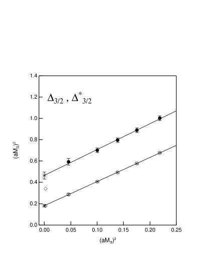
Figure 5: Squared masses of $\Delta$ baryons ($J^{P}=3/2^{\pm}$) in lattice unit as functions of squared pion mass. All symbols are defined as in Figure 4.

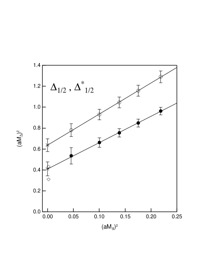
Figure 6: Squared masses of $\Delta$ baryons ($J^{P}=1/2^{\pm}$) in lattice unit as functions of squared pion mass. All symbols are defined as in Figure 4.

In Figs. 4-6, we show squared masses of positive- and negative-parity baryons as a function of squared pion mass in each ($I$, $J$) channel. Circle symbols correspond to the negative-parity state (solid circles) and the positive-parity state (open circles). The extrapolated points in the chiral limit are represented by star symbols. In Table 9, respective values in the chiral limit for all calculated baryons are listed and also compared with experimental values. Two types of input ($r_{0}$ input and $M_{\rho}$ input) are taken to expose the dependence on the choice of input to set a scale. We should keep in mind that the systematic errors stemming from this dependence are around 5%, the value of which exceeds the amount of the statistical errors in the case of the nucleon and the $\Delta_{3/2}$. Instead, we quote various mass ratios, which do not suffer from such systematic uncertainties:

$$\begin{array}[]{rclr}M_{\Delta_{3/2}}/M_{N}&=&1.28(4)(9)&({\rm Expt.:}\;\sim 1.31)\\ M_{N^{*}}/M_{N}&=&1.61(10)(16)&({\rm Expt.:}\;\sim 1.63)\\ M_{\Delta^{*}_{3/2}}/M_{N^{*}}&=&1.28(7)(7)&({\rm Expt.:}\;\sim 1.11)\\ M_{\Delta^{*}_{3/2}}/M_{\Delta_{3/2}}&=&1.61(7)(13)&({\rm Expt.:}\;\sim 1.38)\end{array}$$

where the second quoted errors correspond to the systematic errors, which are estimated from the difference in the central values obtained by two types of chiral extrapolation. The mass ratio between the nucleon and its parity partner (or its hyperfine partner) shows a good agreement with the experimental values within statistical errors. However, mass ratios that include $M_{\Delta_{3/2}^{*}}$ are overestimated by about 15%. Our calculations are performed using the relatively heavy quark masses ($M_{\pi}/M_{\rho}\sim 0.66-0.96$). The long chiral extrapolation is performed so that the evaluated values should not be taken too seriously. Indeed, both the “linear” fit and the “curve” fit do not include a term linear in $aM_{\pi}$, which is responsible for the expected leading behavior close to the chiral limit in the quenched approximation. Labrenz:1996jy

Finally we stress that the level ordering in $\Delta$ spectra , $M_{\Delta_{3/2}}<M_{\Delta^{*}_{1/2}}\mathrel{\hbox to0.0pt{\raise 2.20013pt\hbox{$<$}\hss}{\lower 2.20013pt\hbox{$\sim$}}}M_{\Delta^{*}_{3/2}}<M_{\Delta_{1/2}}$, is well reproduced in comparison to corresponding $\Delta$ states, which are all ranked as four stars on the Particle Data Table Eidelman:2004wy . In addition, it is worth mentioning that a signal of $\Delta(1750)$ ($I=3/2$ and $J^{P}=1/2^{+}$), which is the weakly established state (one star) Eidelman:2004wy , cannot be seen in our data.

III.3 Hyperfine mass splitting

In this subsection, we discuss our numerical results on the hyperfine mass splittings in both parity channels (e.g. $M_{\Delta_{3/2}}-M_{N}$ and $M_{\Delta_{3/2}^{*}}-M_{N^{*}}$). In the quark potential model, if the inter-quarks potential is central force and independent of the flavor and spin, the hamiltonian has spin-flavor $SU(6)$ symmetry Capstick:2000qj . Under the exact spin-flavor $SU(6)$ symmetry, masses of resonance in the same $SU(6)$ multiplet, e.g. ${\bf 56}$-plet for the nucleon and the $\Delta_{3/2}$ particle or ${\bf 70}$-plet for negative-parity $N^{*}$ and $\Delta_{3/2}^{*}$ states, should be degenerate. However, the actual baryon spectra show evident violations of this symmetry. In the non-relativistic quark models, violations of the spin-flavor $SU(6)$ symmetry are caused by spin-dependent interactions Capstick:2000qj .

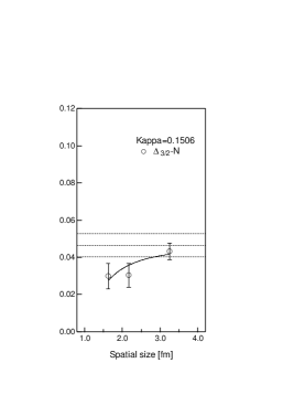
Figure 7: Masses of spin-1/2 $\Delta$ baryons in lattice unit as functions of spatial lattice size in the physical unit for $\kappa=0.1506$ (left figure) and $\kappa=0.1497$ (right figure). Solid curves are fits of the form $aM_{L}=aM_{\infty}+cL^{-n}$ with the value $n=2$. Horizontal dashed lines represent the mean value of the infinite volume extrapolation and one standard deviation from it.

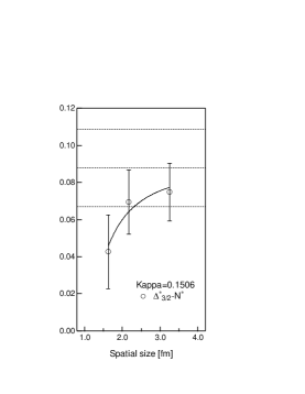
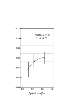
Figure 8: Masses of spin-1/2 $\Delta$ baryons in lattice unit as functions of spatial lattice size in the physical unit for $\kappa=0.1506$ (left figure) and $\kappa=0.1497$ (right figure). Solid curves and dashed lines are defined as in Figure 7.

First, we consider the finite-size effect on the hyperfine mass splittings ($N-\Delta_{3/2}$ and $N^{*}-\Delta_{3/2}^{*}$). The lattice-size dependences of the hyperfine mass splittings are shown in Figs. 7 and 8. We observe an unique feature in both parity channels. Each hyperfine splitting becomes small as the spatial lattice size decreases . This feature is rather peculiar from the viewpoint of the non-relativistic quark models. The hyperfine interaction may be derived from one-gluon exchange as a spin-spin component of the Fermi-Breit type interaction. Thus, the hyperfine mass splitting originates from a contact interaction between colored quarks Capstick:2000qj . As the size of a hadron decreases, probability of finding two quarks at the same spatial point inside hadron increases, so that the hyperfine mass splitting would increase. However, the observed finite-size effect where the hyperfine mass splitting diminishes as the lattice size decreases is opposite from above naive expectation. At present, we do not have a simple interpretation of the finite-size behavior of the hyperfine mass splitting in our data of quenched lattice QCD. This peculiar behavior may suggest some other origin of the hyperfine interaction Capstick:2000qj rather than one-gluon exchange. Finally, it is worth mentioning that the observed size dependence of the hyperfine mass splitting accounts for the opposite pattern of the finite-size effect on masses of the $\Delta_{3/2}$ and also our observation that the finite-size effect for the $\Delta_{3/2}^{*}$ state is slightly milder than the $N^{*}$ state.

We shortly comment on the splittings between pairs of parity partner ($N-N^{*}$ and $\Delta_{3/2}-\Delta_{3/2}^{*}$). It is found that these splittings become small as the lattice size decreases in both $N$ and $\Delta$ channels. All data including hyperfine mass splittings are tabulated in Table 10.

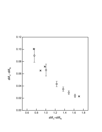
Figure 9: Hyperfine splitting between the $N$ and $\Delta_{3/2}$ states as a function of $M_{\Delta}+M_{N}$. All calculations are done for three degenerate valence-quarks. The experimental values in the wide range from the light (up, down) sector to the charm sector are marked by stars.

Next, we discuss the quark-mass dependence of the hyperfine mass splitting. In Fig. 9, the hyperfine mass splittings between the nucleon and the $\Delta_{3/2}$ are plotted as a function of sum of the nucleon and $\Delta_{3/2}$ masses by using data at the largest spatial lattice size, $La\simeq 3.2$ fm. We find that the hyperfine mass splitting becomes large as the quark mass decreases. This feature shows a good agreement with the general form of the spin-dependent interaction in the non-relativistic quark models where the spin-dependent interaction is proportional to inverse powers of the quark mass Capstick:2000qj . Of course, one can easily find such the feature in the actual baryon spectra in the wide range from the light (up, down) sector to the charm sector. Fig. 9 includes some experimental points (stars), which correspond to spin 1/2 and 3/2 doublets; $N(939)-\Delta(1232)$, $\Sigma(1192)-\Sigma(1385)$, $\Xi(1315)-\Xi(1530)$ and $\Sigma_{c}(2455)-\Sigma_{c}(2520)$. Our data including the chiral extrapolated value, $M_{\Delta_{3/2}}-M_{N}=0.262(11)$ GeV, is fairly consistent with those experimental points. It is also found that the quark-mass dependence for the hyperfine mass splitting between the $\Delta_{3/2}^{*}$ and the $N^{*}$ is consistent with the naive expectation, which is deduced from the explicit mass dependence of the spin-dependent interaction in the non-relativistic quark models.

Finally, it is important to note that the value of the hyperfine mass splitting should be sensible to the leading discretization errors of the Wilson fermion action, which may induce the extra chromomagnetic-moment interaction at finite lattice spacing. We however believe that qualitative features of the finite-size dependence and the quark-mass dependence, which are observed in this paper, do not change with respect to discretization ${\cal O}(a)$ errors.

IV Conclusions

In this paper, we have studied the finite-size effect on masses of various baryons: the nucleon states in both parity channels ($J^{P}=1/2^{\pm}$) and the $\Delta$ states in all spin-parity channels ($J^{P}=1/2^{\pm},3/2^{\pm}$). Our quenched lattice simulations were employed at relatively weaker coupling, $\beta=6/g^{2}=6.2$, where the cut-off scale ($\sim 3$ GeV) is definitely higher than mass scale of all observed baryons ($\sim 1-2$ GeV). Three different lattice sizes, $La\simeq 1.6,2.2$ and 3.2 fm, were utilized to examine how large lattice size is required for excited baryon spectroscopy.

We have found the considerable finite-size effect on masses of all $\Delta$ states and negative-parity nucleon $N^{*}$ even in the relatively heavy quark region where the finite-size effect on the nucleon is almost negligible. The finite-size behavior that we observed can be described by a power law $M_{\infty}-M_{L}\propto L^{-n}$ with $n\approx 2$ rather than the exponential form $\propto L^{-1}\exp(-L/L_{0})$. This observation is consistent with that reported in Ref Fukugita:1992jj . If the finite-size effect is kept as small as a few percent level, the spatial lattice size $La\mathrel{\hbox to0.0pt{\raise 2.20013pt\hbox{$>$}\hss}{\lower 2.20013pt\hbox{$\sim$}}}3$ fm should be required for excited baryons, especially for the negative-parity nucleon.

The finite-size behavior of the power law might originate from the phenomenological point of view as the squeezed hadron size. Indeed, we confirmed that the rather large finite-size effect appears for excited baryons, the “wave function” of which ought to be extended rather than that of the ground state. The squeezed “wave function” may increase the total energy of the three-quark system because of a gain in kinetic energy of internal quarks inside hadron so that the mass is expected to be pushed up as the lattice size decreases. However, the $\Delta_{3/2}$ state, which is the lowest lying state in the $\Delta$ channel, reveals the opposite pattern of the size effect. The mass of the $\Delta_{3/2}$ decreases as the lattice size decreases. This peculiar behavior might attribute to the finite-size effect on the hyperfine interaction.

According to the $SU(6)$ quark model, the nucleon and the $\Delta_{3/2}$ belong to the same $SU(6)$ multiplet so that the difference of wave functions between the $N$ and the $\Delta_{3/2}$ is induced by the hyperfine interaction. Our study of the finite-size effect were performed in the relatively heavy quark mass region, where the finite-size effect on the nucleon mass is almost negligible. Therefore, the finite-size effects on the $\Delta_{3/2}$ can attribute to the effect of the hyperfine mass splitting. Indeed, in the case of the $N^{*}-\Delta^{*}_{3/2}$ hyperfine mass splitting, we observed the same pattern of the finite-size effect where $N^{*}-\Delta^{*}_{3/2}$ splitting diminishes as the lattice spatial size decreases, while either $N^{*}$ or $\Delta^{*}_{3/2}$ states yield the expected size effect where both masses increase as the lattice size decreases. However, the hyperfine interaction induced by one-gluon exchange, which is mainly a contact interaction between colored quarks, may not correctly account for this peculiar behavior of the finite-size effect. It seems that our observed finite-size effect on the hyperfine mass splitting suggests some other origin of the hyperfine interaction for baryons rather than one-gluon exchange.

Appendix A (anti-)periodic time dependence for finite T

Let us consider the functional form of the typical two-point correlation function $G(t)=e^{-M|t|}$ under the periodic (anti-periodic) boundary condition in time. The desired function, in the finite extent $T$ with the periodic boundary condition, should be formed as

$$G_{\rm p.b.c.}(t)=\sum_{n=-\infty}^{\infty}G(t+nT),$$ (26)

which certainly satisfies $G_{\rm p.b.c.}(t)=G_{\rm p.b.c.}(t+T)$. Recall that the given correlation function $G(t)$ clearly has the time-reflection symmetry $G(t)=G(-t)$. Thus, one can rewrite $G_{\rm p.b.c.}(t)$ for $0\leq t<T$ as

$$G_{\rm p.b.c.}(t) = \sum_{n=0}^{\infty}G(t+nT)+\sum_{n=1}^{\infty}G(nT-t)$$ (27)

$$= \sum_{n=0}^{\infty}e^{-M(t+nT)}+\sum_{n=1}^{\infty}e^{-M(nT-t)}$$

$$= \sum_{n=0}^{\infty}e^{-nMT}\left[e^{-Mt}+e^{-M(T-t)}\right].$$

In the case of the anti-periodic boundary condition, where $G_{\rm a.p.b.c.}(t)=-G_{\rm a.p.b.c.}(t+T)$, one obtains the following general form:

$$G_{\rm a.p.b.c.}(t) = \sum_{n=-\infty}^{\infty}(-)^{n}G(t+nT)$$ (28)

$$= \sum_{n=0}^{\infty}(-)^{n}G(t+nT)+\sum_{n=1}^{\infty}(-)^{n}G(nT-t)$$

$$= \sum_{n=0}^{\infty}(-)^{n}e^{-nMT}\left[e^{-Mt}-e^{-M(T-t)}\right].$$

We would like to make the following few comments. First, we can derive familiar forms from Eqs.(27) and (28) as the asymptotic form in the large $T$ limit ($MT>>1$).

$$G_{\rm p.b.c./a.p.b.c.}(t)\rightarrow e^{-Mt}\pm e^{-M(T-t)}$$

which has only a contribution from the first wrap-round effect. The $(n-1)$-th wrap-round effect should be suppressed with the factor $e^{-nMT}$. Then, the linear combination of $G_{\rm p.b.c.}(t)$ and $G_{\rm a.p.b.c.}(t)$ yields

$$\overline{G}(t)=\frac{1}{2}\left[G_{\rm p.b.c.}(t)+G_{\rm a.p.b.c.}(t)\right]\approx e^{-Mt}$$

where the first wrap-round effect is canceled.

Secondary, we will see that $\overline{G}(t)$ corresponds to a periodic function in the finite extent $2T$ as follows. One sums up all wrap-round contributions in Eqs.(27) and (28), and then obtains the exact functional forms:

$$G_{\rm p.b.c.}(t) = \frac{1}{1-e^{-MT}}\left[e^{-Mt}+e^{-M(T-t)}\right]=\frac{\cosh[M(t-\frac{T}{2})]}{\sinh[M\frac{T}{2}]}$$ (29)

$$G_{\rm a.p.b.c.}(t) = \frac{1}{1+e^{-MT}}\left[e^{-Mt}-e^{-M(T-t)}\right]=-\frac{\sinh[M(t-\frac{T}{2})]}{\cosh[M\frac{T}{2}]}$$ (30)

where the (anti-)periodic time dependence for finite $T$ is given by a $\cosh(\sinh)$ function. Therefore, $\overline{G}(t)$ is given by

$$\overline{G}(t)=\frac{1}{2}\left(\frac{\cosh[M(t-\frac{T}{2})]}{\sinh[M\frac{T}{2}]}-\frac{\sinh[M(t-\frac{T}{2})]}{\cosh[M\frac{T}{2}]}\right)=\frac{\cosh[M(t-T)]}{\sinh[MT]}$$ (31)

The final expression is nothing but $G_{\rm p.b.c.}(t)$ with the $2T$-periodicity.

Table 1: Simulation parameters for each volume studied in this work.

$\beta$	lattice size ($L^{3}\times T$)	kappa values	statistics	$\sim La$ (fm)
6.2	$24^{3}\times 48$	{0.1506, 0.1497}	320	1.6
	$32^{3}\times 48$	{0.1506, 0.1497}	240	2.2
	$48^{3}\times 48$	{0.1520, 0.1506, 0.1497, 0.1489, 0.1480}	210	3.2

Table 2: The physical scale set by the Sommer parameter $r_{0}=0.5$ fm. The value of $r_{0}/a$ is taken from Ref. Guagnelli:1998ud .

$\beta$	$r_{0}/a$	$a^{-1}$ (GeV)	$a$ (fm)
6.2	7.380(3)	2.913	0.06775

Table 3: Finite-size effect on masses of all measured baryons at $\beta=6.2$

$L^{3}\times T$	$\kappa$	$aM_{N}$	$aM_{N^{*}}$	$aM_{\Delta_{3/2}}$	$aM_{\Delta_{3/2}^{*}}$	$aM_{\Delta_{1/2}}$	$aM_{\Delta_{1/2}^{*}}$
$24^{3}\times 48$	0.1506	0.594(5)	0.829(19)	0.624(7)	0.872(16)	0.993(24)	0.777(28)
	0.1497	0.667(4)	0.891(15)	0.693(5)	0.928(13)	1.055(22)	0.864(22)
$32^{3}\times 48$	0.1506	0.597(4)	0.808(15)	0.628(7)	0.878(13)	0.985(27)	0.835(25)
	0.1497	0.670(3)	0.873(13)	0.697(4)	0.928(12)	1.043(25)	0.901(21)
$48^{3}\times 48$	0.1506	0.594(4)	0.762(15)	0.637(5)	0.837(14)	0.964(26)	0.814(28)
	0.1497	0.668(3)	0.832(13)	0.702(4)	0.892(12)	1.023(25)	0.869(23)

Table 4: Infinite volume limit of various baryon masses at $\beta=6.2$

$\kappa$	type	$aM_{N}$	$\chi^{2}/N_{DF}$	$aM_{N^{*}}$	$\chi^{2}/N_{DF}$	$aM_{\Delta_{3/2}}$	$\chi^{2}/N_{DF}$	$aM_{\Delta_{3/2}^{*}}$	$\chi^{2}/N_{DF}$
0.1506	$L^{-3}$	0.597(4)	0.46	0.763(16)	1.54	0.638(5)	0.42	0.846(14)	3.06
	$L^{-2}$	0.595(5)	0.47	0.747(20)	0.94	0.641(7)	0.26	0.836(18)	2.56
	$L^{-1}$	0.595(9)	0.47	0.697(36)	0.45	0.651(12)	0.12	0.808(31)	2.01
0.1497	$L^{-3}$	0.669(4)	0.37	0.833(13)	1.70	0.703(4)	0.22	0.898(12)	2.51
	$L^{-2}$	0.669(5)	0.40	0.819(17)	1.06	0.705(6)	0.11	0.889(16)	2.00
	$L^{-1}$	0.669(8)	0.41	0.775(30)	0.52	0.712(10)	0.03	0.862(27)	1.47

Table 5: Summary table of the finite-size effect on various baryon masses for $\kappa=0.1506$.

baryon	as increase $L$	$\sim(M_{\mathrm{1.6\hskip 2.0ptfm}}-M_{\infty})/M_{\infty}$	$\sim|M_{\mathrm{3.2\hskip 2.0ptfm}}-M_{\infty}|/M_{\infty}$
$N$	$\to$	less than $1\%$	less than $1\%$
$N^{*}$	$\searrow$	$11\%$	$2\%$
$\Delta_{3/2}$	$\nearrow$	$-3\%$	less than $1\%$
$\Delta_{3/2}^{*}$	$\searrow$	$4\%$	less than $1\%$

Table 6: Fitted masses of pion, $\rho$-meson and nucleon ($J^{P}=1/2^{\pm}$) states at $\beta=6.2$ and lattice volume $48^{3}\times 48$.

$\kappa$	$aM_{\pi}$	range	$aM_{\rho}$	range	$aM_{N}$	range	$aM_{N^{*}}$	range
$\kappa_{c}$	0	N/A	0.248(3)	N/A	0.332(9)	N/A	0.534(33)	N/A
0.1520	0.2141(8)	[15,30]	0.324(2)	[14,30]	0.469(5)	[20,28]	0.640(22)	[13,20]
0.1506	0.3167(9)	[15,30]	0.388(1)	[14,30]	0.594(4)	[20,28]	0.762(15)	[13,20]
0.1497	0.3726(9)	[15,30]	0.430(1)	[14,30]	0.668(3)	[20,28]	0.832(13)	[13,20]
0.1489	0.4188(9)	[15,30]	0.467(1)	[14,30]	0.730(3)	[20,28]	0.891(12)	[13,20]
0.1480	0.4678(9)	[15,30]	0.509(1)	[14,30]	0.799(3)	[20,28]	0.957(11)	[13,20]

Table 7: Fitted masses of $\Delta$ baryons ($J^{P}=3/2^{\pm},1/2^{\pm}$) at $\beta=6.2$ and lattice volume $48^{3}\times 48$.

$\kappa$	$aM_{\Delta_{3/2}}$	range	$aM_{\Delta_{3/2}^{*}}$	range	$aM_{\Delta_{1/2}}$	range	$aM_{\Delta_{1/2}^{*}}$	range
$\kappa_{c}$	0.424(11)	N/A	0.681(25)	N/A	0.798(38)	N/A	0.640(53)	N/A
0.1520	0.535(9)	[22,28]	0.770(21)	[12,20]	0.883(34)	[10,15]	0.732(54)	[13,20]
0.1506	0.637(5)	[22,28]	0.837(14)	[12,20]	0.964(26)	[10,15]	0.814(28)	[13,20]
0.1497	0.702(4)	[22,28]	0.892(12)	[12,20]	1.023(25)	[10,15]	0.869(23)	[13,20]
0.1489	0.759(4)	[22,28]	0.943(12)	[12,20]	1.076(25)	[10,15]	0.921(20)	[13,20]
0.1480	0.822(4)	[22,28]	1.001(11)	[12,20]	1.136(25)	[10,15]	0.981(18)	[13,20]

Table 8: Results of the chiral extrapolated masses in lattice units for all measured hadrons by two types of fitting formula, the linear and curve fits.

type		$aM_{\rho}$	$aM_{N}$	$aM_{N^{*}}$	$aM_{\Delta_{3/2}}$	$aM_{\Delta_{3/2}^{*}}$	$aM_{\Delta_{1/2}}$	$aM_{\Delta_{1/2}^{*}}$
linear	(mass)	0.283(2)	0.403(7)	0.582(26)	0.477(8)	0.703(22)	0.818(35)	0.670(44)
	($\chi^{2}/N_{DF}$)	6.20(1.67)	9.62(3.37)	0.62(0.45)	1.57(0.99)	0.03(0.08)	0.01(0.02)	0.01(0.05)
curve	(mass)	0.248(3)	0.332(9)	0.534(33)	0.424(11)	0.681(25)	0.798(38)	0.640(53)
	($\chi^{2}/N_{DF}$)	1.59(0.63)	0.03(0.14)	0.07(0.12)	0.05(0.15)	0.17(0.21)	0.01(0.03)	0.01(0.05)

Table 9: The third and forth columns list results of all measured baryon masses in GeV units, which are set by two different inputs, $r_{0}$ input and $M_{\rho}$ input. The fifth and sixth list experimental values of the corresponding baryon and its status in the Particle Data Table Eidelman:2004wy . The possible assignments of the $SU(6)\otimes O(3)$ supermultiplet are also embedded into the final column.

state	($I,J^{P}$)	our results [GeV]		physical baryon	(status)	$SU(6)\otimes O(3)$
		($r_{0}$ input)	($M_{\rho}$ input)			classification
$N$	$(\frac{1}{2},\frac{1}{2}^{+})$	0.967(26)	1.030(27)	$N(939)$	****	[56,$0^{+}$]
$N^{*}$	$(\frac{1}{2},\frac{1}{2}^{-})$	1.555(96)	1.658(102)	$N(1535)$ $S_{11}$	****	[70,$1^{-}$]
$\Delta_{3/2}$	$(\frac{3}{2},\frac{3}{2}^{+})$	1.235(32)	1.316(34)	$\Delta(1232)$ $P_{33}$	****	[56,$0^{+}$]
$\Delta^{*}_{3/2}$	$(\frac{3}{2},\frac{3}{2}^{-})$	1.983(72)	2.114(77)	$\Delta(1700)$ $D_{33}$	****	[70,$1^{-}$]
$\Delta_{1/2}$	$(\frac{3}{2},\frac{1}{2}^{+})$	2.324(110)	2.477(117)	$\Delta(1910)$ $P_{31}$	****	[56,$2^{+}$] or [70,$0^{+}$]
$\Delta^{*}_{1/2}$	$(\frac{3}{2},\frac{1}{2}^{-})$	1.864(154)	1.987(164)	$\Delta(1620)$ $S_{31}$	****	[70,$1^{-}$]

Table 10: Finite-size effect on various mass splittings at $\beta=6.2$

$L^{3}\times T$	$\kappa$	$aM_{\Delta_{3/2}}$-$aM_{N}$	$aM_{\Delta_{3/2}^{*}}$-$aM_{N^{*}}$	$aM_{N^{*}}$-$aM_{N}$	$aM_{\Delta_{3/2}^{*}}$-$aM_{\Delta_{3/2}}$	$aM_{\Delta_{1/2}}$-$aM_{\Delta_{1/2}^{*}}$
$24^{3}\times 48$	0.1506	0.030(7)	0.043(20)	0.235(21)	0.248(18)	0.216(36)
	0.1497	0.026(5)	0.037(14)	0.224(16)	0.235(15)	0.191(30)
$32^{3}\times 48$	0.1506	0.030(6)	0.070(17)	0.211(17)	0.250(15)	0.150(37)
	0.1497	0.027(4)	0.055(13)	0.201(14)	0.231(13)	0.143(33)
$48^{3}\times 48$	0.1506	0.043(5)	0.075(16)	0.168(18)	0.200(16)	0.151(35)
	0.1497	0.035(4)	0.060(12)	0.164(15)	0.190(14)	0.154(31)

References

- (1) F. X. Lee and D. B. Leinweber, Nucl. Phys. Proc. Suppl. 73, 258 (1999). S. Sasaki, Nucl. Phys. Proc. Suppl. 83, 206 (2000) and hep-ph/0004252.
- (2) S. Sasaki, T. Blum and S. Ohta, Phys. Rev. D 65, 074503 (2002).
- (3) M. Gockeler, R. Horsley, D. Pleiter, P. E. Rakow, G. Schierholz, C. M. Maynard and D. G. Richards, Phys. Lett. B 532, 63 (2002).
- (4) W. Melnitchouk, S. Bilson-Thompson, F. D .R. Bonnet, J.N. Hedditch, F. X. Lee, D. B. Leinweber, A. G. Williams, J. M. Zanotti and J. B. Zhang, Phys. Rev. D 67, 114506 (2003).
- (5) J. M. Zanotti, D. B. Leinweber, A. G. Williams, J. B. Zhang, W. Melnitchouk and S. Choe, Phys. Rev. D 68, 054506 (2003).
- (6) Y. Nemoto, N. Nakajima, H. Matsufuru and H. Suganuma, Phys. Rev. D 68, 094505 (2003).
- (7) N. Mathur, Y. Che, S. J. Dong, T. Draper, I. Horvath, F. X. Lee, K. F. Liu, J. B. Zhang, Phys. Lett. B 605, 137 (2005).
- (8) D. Brommel, P. Crompton, C. Gattringer, L. Y. Glozman, C. B. Lang, S. Schaefer and A. Schafer, Phys. Rev. D 69, 094513 (2004).
- (9) T. Burch, C. Gattringer, L. Y. Glozman, R. Kleindl, C. B. Lang and A. Schaefer, Phys. Rev. D 70, 054502 (2004).
- (10) D. Guadagnoli, M. Papinutto and S. Simula, Phys. Lett. B 604, 74 (2004).
- (11) For a review, see D. B. Leinweber, W. Melnitchouk, D. G. Richards, A. G. Williams and J. M. Zanotti, nucl-th/0406032.
- (12) M. Lüscher, Commun. Math. Phys. 104, 177 (1986).
- (13) M. Fukugita, H. Mino, M. Okawa, G. Parisi and A. Ukawa, Phys. Lett. B 294, 380 (1992).
- (14) R. Gupta and A. Patel, Phys. Lett. B 124, 94 (1983).
- (15) G. Martinelli, G. Parisi, R. Petronzio and F. Rapuano, Phys. Lett. B 122, 283 (1983).
- (16) S. Aoki, T. Umemura, M. Fukugita, N. Ishizuka, H. Mino, M. Okawa and A. Ukawa, Phys. Rev. D 50, 486 (1994).
- (17) For a review, see S. Sasaki, hep-lat/0410016.
- (18) S. Sasaki, Phys. Rev. Lett. 93, 152001 (2004).
- (19) S. Sasaki, Prog. Theor. Phys. Suppl. 151, 143 (2003).
- (20) B. L. Ioffe, Nucl. Phys. B 188, 317 (1981) [Erratum-ibid. B 191, 591 (1981)].
- (21) F. Fucito, G. Martinelli, C. Omero, G. Parisi, R. Petronzio and F. Rapuano, Nucl. Phys. B 210, 407 (1982).
- (22) D. B. Leinweber, T. Draper and R. M. Woloshyn, Phys. Rev. D 46, 3067 (1992).
- (23) M. Benmerrouche, R. M. Davidson and N. C. Mukhopadhyay, Phys. Rev. C 39 (1989) 2339.
- (24) A. Frommer, V. Hannemann, B. Nockel, T. Lippert and K. Schilling, Int. J. Mod. Phys. C 5, 1073 (1994).
- (25) S. Choe, S. Muroya, A. Nakamura, C. Nonaka, T. Saito and F. Shoji, Nucl. Phys. Proc. Suppl. 106, 1037 (2002).
- (26) M. Guagnelli, R. Sommer and H. Wittig Nucl. Phys. B 535, 389 (1998). S. Necco and R. Sommer, Nucl. Phys. B 622, 328 (2002).
- (27) J. N. Labrenz and S. R. Sharpe, Phys. Rev. D 54, 4595 (1996).
- (28) S. Eidelman et al. [Particle Data Group], Phys. Lett. B 592 (2004) 1.
- (29) For a review, see S. Capstick and W. Roberts, Prog. Part. Nucl. Phys. 45, S241 (2000).
- (30) S. Choe et al., JHEP 0308, 022 (2003).
Acknowledgments
It is a pleasure to acknowledge A. Nakamura and C. Nonaka for helping us develop codes for our lattice QCD simulations from their open source codes (Lattice Tool Kit Choe:2002pu ). We also appreciate T. Hatsuda for helpful suggestions. This work is supported by the Supercomputer Projects No.102 (FY2003) and No.110 (FY2004) of High Energy Accelerator Research Organization (KEK). S.S. thanks for the support by JSPS Grand-in-Aid for Encouragement of Young Scientists (No.15740137).