Entropy of spatial monopole currents in pure SU(2) QCD at finite temperature

Abstract

We study properties of space–like monopole trajectories in the Maximal Abelian gauge of quenched SU(2) QCD at the finite temperature. We concentrate on infrared monopole clusters which are responsible for the confinement properties of the theory. We determine numerically the effective action of the monopoles projected onto the three-dimensional time–slice. Then we derive the length distributions of the monopole loops and fix their entropy.

I Introduction

The interest in the Abelian monopoles in the non–Abelian gauge theories is motivated by a central role of these objects in the dual superconductor mechanism DualSuperconductor of color confinement. The Abelian monopoles can be considered as particular configurations of gluon fields with magnetic quantum numbers. In pure non–Abelian gauge theories the Abelian monopoles do not exist at the classical level. However, these topological defects can successfully be identified given a dynamical configuration of the gluon fields in a particular Abelian gauge AbelianProjections . There are many Abelian gauges among which the most popular one is the Maximal Abelian (MA) gauge kronfeld . In this gauge the off-diagonal gluon fields are suppressed and short–ranged contrary to the diagonal (Abelian) gluon fields ref:propagators . There are many numerical experiments confirming that Abelian degrees of freedom are responsible for the confinement of color (for a review, see Ref. Reviews ). In particular, it was observed in Refs. AbelianDominance ; shiba:string that the tension of the chromoelectric string is dominated by the Abelian monopole contributions. Moreover, the monopole condensate – which guarantees the formation of the chromoelectric string between the quarks – exists in the confinement phase and disappears in the deconfinement phase shiba:condensation ; MonopoleCondensation .

The trajectories of the Abelian monopoles form two different types of clusters. A typical configuration contains a lot of finite-sized clusters and one large percolating cluster ivanenko ; ref:kitahara . The percolating cluster (or, the infrared (IR) cluster) occupies the whole lattice while the sizes of the other clusters have an ultraviolet nature. The monopole condensate corresponds to the so-called percolating (infrared) cluster of the monopole trajectories. The tension of the confining string gets a dominant contribution from the IR monopole cluster ref:kitahara while the finite-sized ultraviolet (UV) clusters do not play any role in the confinement. Various properties of the UV and IR monopole clusters were investigated previously in Refs. ref:kitahara ; ref:clusters ; IshiguroSuzuki .

At high temperatures the Abelian monopoles become static. In the high temperature phase the IR monopole cluster disappears ivanenko ; ref:kitahara and, consequently, the confinement of the static quarks is lost. Since the static currents do not play any role in confinement we concentrate below on the spatial components of the IR monopole cluster. We investigate the action, the length distribution and the entropy of spatial components of the infrared monopole clusters. We follow Ref. IshiguroSuzuki where energy and entropy of the monopole currents were studied at zero temperature. Our preliminary results were reported in Ref. IshiguroSuzuki:spatial:Lattice .

The plan of the paper is as follows. In Section II we describe the model and provide the description of the monopole currents. The details of numerical simulations are also given in this Section. Section III is devoted to the investigation of the Abelian monopole action obtained by the inverse Monte-Carlo method for the clusters of the spatially projected Abelian monopoles. In Section IV we study the length distributions of the infrared clusters of the spatially projected monopole clusters. The knowledge of the monopole action and cluster distribution allows us to calculate the entropy of the spatial monopole currents which is discussed in Section V. Our conclusions are presented in the last Section.

II Model

We study pure SU(2) QCD with the standard Wilson lattice action for gluon fields,

$$S(U)=-\frac{\beta}{2}{\mathrm{Tr}}\sum_{P}U_{P}\,,$$ (1)

where $\beta$ is the coupling constant, the sum goes over all plaquettes of the lattice, and $U_{P}\equiv U_{s,\mu\nu}=U_{s,\mu}U_{s+\hat{\mu},\nu}U^{\dagger}_{s+\hat{\nu},\mu}U^{\dagger}_{s,\nu}$ is the SU(2) plaquette constructed from link fields, $U_{s,\mu}$. We work in the MA gauge kronfeld defined by the maximization of the lattice functional

$$R=\sum_{s,\hat{\mu}}{\mathrm{Tr}}\Big{(}\sigma_{3}\widetilde{U}(s,\mu)\sigma_{3}\widetilde{U}^{\dagger}(s,\mu)\Big{)}\,,$$ (2)

with respect to the gauge transformations $U(s,\mu)\to\widetilde{U}(s,\mu)=\Omega(s)U(s,\mu)\Omega^{\dagger}(s+\hat{\mu})$. In the continuum limit the local condition of maximization (2) can be written in terms of the differential equation, $(\partial_{\mu}+igA_{\mu}^{3})(A_{\mu}^{1}-iA_{\mu}^{2})=0$. Both this condition and the functional (2) are invariant under residual U(1) gauge transformations, $\Omega^{\mathrm{Abel}}(\omega)={\mathrm{diag}(e^{i\omega(s)},e^{-i\omega(s)})}$.

After the Abelian gauge is fixed we perform the projection of the non-Abelian gauge fields, $U_{s,\mu}$, onto the Abelian ones, $u_{s,\mu}$:

$$\widetilde{U}(s,\mu)=\left(\begin{array}[]{cc}(1-|c(s,\mu)|^{2})^{1/2}&-c^{*}(s,\mu)\\ c(s,\mu)&(1-|c(s,\mu)|^{2})^{1/2}\end{array}\right)\left(\begin{array}[]{cc}u(s,\mu)&0\\ 0&u^{*}(s,\mu)\end{array}\right),$$ (7)

where $c(s,\mu)$ corresponds to the charged (off-diagonal) matter fields.

As we have discussed above, the dominant information about the confinement properties of the theory is located in the monopole configurations which are identified with the help of the Abelian phases of the diagonal fields, $\theta_{s,\mu}$. The Abelian field strength $\theta_{\mu\nu}(s)\in(-4\pi,4\pi)$ is defined on the lattice plaquettes by a link angle $\theta(s,\mu)\in[-\pi,\pi)$ as $\theta_{\mu\nu}(s)=\theta(s,\mu)+\theta(s+\hat{\mu},\nu)-\theta(s+\hat{\nu},\mu)-\theta(s,\nu)$. The field strength $\theta_{\mu\nu}(s)$ can be decomposed into two parts,

$$\theta_{\mu\nu}(s)=\bar{\theta}_{\mu\nu}(s)+2\pi m_{\mu\nu}(s)\,,$$ (8)

where $\bar{\theta}_{\mu\nu}(s)\in[-\pi,\pi)$ is interpreted as the electromagnetic flux through the plaquette and $m_{\mu\nu}(s)$ can be regarded as a number of the Dirac strings piercing the plaquette.

The elementary monopole current can conventionally be constructed using the DeGrand-Toussaintdegrand definition:

$$k_{\mu}(s) = \frac{1}{2}\epsilon_{\mu\nu\rho\sigma}\partial_{\nu}m_{\rho\sigma}(s+\hat{\mu}),$$ (9)

where $\partial$ is the forward lattice derivative. The monopole current is defined on a link of the dual lattice and takes the values $0,\pm 1,\pm 2$. Moreover the monopole current satisfies the conservation law automatically,

$$\partial^{\prime}_{\mu}k_{\mu}(s)=0\,,$$ (10)

where $\partial^{\prime}$ is the backward derivative on the dual lattice.

The monopole current (9) corresponds to the monopole charge defined on the scale of the elementary lattice spacing, $a$. Obviously, the scale $a$ becomes smaller as we approach the continuum limit. In order to study the properties of the monopoles at fixed physical scales we use the so–called extended monopoles ivanenko . The $n^{3}$ extended monopole is defined on a coarse sublattice with the lattice spacing $b=na$. Thus the construction of the extended monopoles corresponds to a block–spin transformation of the monopole currents with the scale factor $n$,

$$k_{\mu}^{(n)}(s)=\sum_{i,j,l=0}^{n-1}k_{\mu}(ns+(n-1)\hat{\mu}+i\hat{\nu}+j\hat{\rho}+l\hat{\sigma})\,.$$ (11)

Since the time–like monopole currents are not essential for the confinement properties we concentrate on the spatial components of the currents. Namely, we investigate spatially projected currents,

$$K_{i}^{(n)}(\vec{s})=\sum^{L_{t}-1}_{s_{4}=0}\,k_{i}^{(n)}(s,s_{4})\,,\,\,i=1,2,3\,,$$ (12)

which are integer–valued and closed.

Technically, we generate 2000-10000 configurations of the SU(2) gauge field, $U$, for $\beta=2.3\sim 2.6$ on the lattices $L_{s}^{3}\times L_{t}$, with $L_{s}=24,32,48,72$ and $L_{t}=4,6,8,12,16$. The number of generated configuration depends on the value of $\beta$ and lattice volume. We fix the gauge with the help of the usual iterative algorithm. In this paper we used the same methods as in the zero–temperature case studied in Ref. IshiguroSuzuki . Thus we refer an interested reader to Ref. IshiguroSuzuki for a more detailed description of the numerical procedures. Below we concentrate on the description of the numerical results.

III Monopole action

In what follows we discuss an effective model of the monopole currents corresponding to pure SU(2) QCD. Formally, we get this effective model through the gauge fixing procedure applied to the original model. Then we integrate out all degrees of freedom but the monopole ones. An effective monopole action is related to the original non-Abelian action $S[U]$ as follows:

$$Z = \int{\cal D}U\,\delta(X)\Delta_{FP}(U)\,e^{-S[U]}=\Bigl{(}\prod_{s,\mu}\sum_{k_{\mu}(s)=-\infty}^{\infty}\Bigr{)}\Bigl{(}\prod_{s}\delta_{\partial_{\mu}^{\prime}k_{\mu}(s),0}\Bigr{)}e^{-S^{{\mathrm{mon}}}_{{\mathrm{eff}}}[k]}\,.$$ (13)

We omit irrelevant constant terms in front of the partition function. The term $\delta(X)$ represents the gauge-fixing condition and $\Delta_{FP}(U)$ is the corresponding Faddeev-Popov determinant. As we have discussed above, the MA gauge fixing condition is given by a maximization of the functional (2) and therefore the local condition $X=0$, implied in Eq. (13), is used here as a formal simplified notation.

Numerically, the monopole action of the $3D$ projected IR monopole clusters can be defined using the inverse Monte–Carlo method shiba:condensation . The action is represented in a truncated form shiba:condensation ; chernodub as a sum of the $m$–point ($m\geq 2$) operators $S_{i}$:

$$S_{{\mathrm{mon}}}[K]=\sum\nolimits_{i}f_{i}S_{i}[K]\,,$$ (14)

where $f_{i}$ are the coupling constants. Following Ref. IshiguroSuzuki we adopt only the two–point interactions in the monopole action, $S_{i}\sim K_{i}(s)K_{j}(s^{\prime})$.

Similarly to the $4D$ case we find that the monopole action of the spatially projected currents is proportional with a good accuracy to the length $L[K]$ of the monopole loop $K$,

$$S_{{\mathrm{mon}}}[K]\backsimeq f_{0}L[K]+const\,.$$ (15)

The important property of the monopole action is that the couplings $f_{i}$ are the functions of the scale $b=na$, Eq. (11), at which the monopole charge is defined. To illustrate this fact we show the dependence of the coupling constant $f_{0}$ on $b=n\,a(\beta)$ in Figure 1.

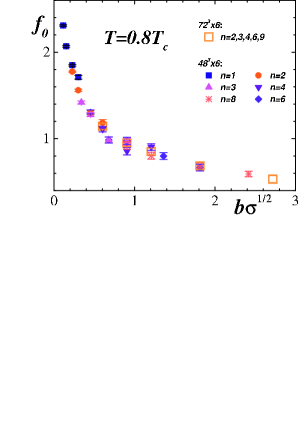
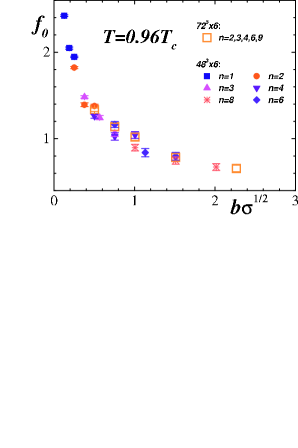
(a)	(b)

Figure 1: The coefficient $f_{0}$ of the monopole action (15) vs. the scale parameter $b$ for the lattice sizes $L_{s}^{3}\times 6$, $L_{s}=48,72$ and blocking factors, $n=1\dots 9$, at temperatures (a) $T=0.8\,T_{c}$ and (b) $T=0.96\,T_{c}$.

From Figure 1 one observes the almost perfect scaling: the parameter $b$ does not depend on the parameters $n$ and $a$ separately. The action is near to the renormalized trajectory which corresponds to the continuum effective action. Moreover, the result does not depend on the spatial extension of the lattice, $L_{s}$. Thus the action of the spatially projected monopole current shows the scaling similarly to the action of the unprojected monopoles shiba:condensation ; chernodub .

IV Length distribution

The length distribution of the spatially–projected monopole clusters is shown in Figure 2.

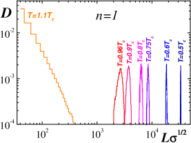
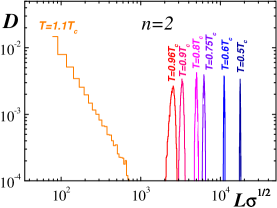
(a)	(b)

Figure 2: The distributions of the spatial monopole currents at various temperatures. For the low temperatures, $T<T_{c}$, the UV–part of the distributions is not shown.

In the confinement phase, $T<T_{c}$, only the infrared part of the distribution is shown. One can see that the length (in physical units) of the monopole trajectory belonging to the percolating cluster becomes shorter as the temperature increases. This fact is expected because the monopole condensate is ”evaporating” as temperature increases towards the transition point, and, therefore, the infrared part of the monopole currents should be more and more diluted.

At $T>T_{c}$ the percolating cluster of the spatially projected currents disappears, and, consequently, the confinement of quarks is lost. The behavior of the elementary and blocked currents is qualitatively the same. According to Ref. IshiguroSuzuki the length of the $4D$ IR monopole currents in the finite volume $V$ is distributed with the Gaussian law, which is in the finite-temperature case can be formulated as follows:

$$D^{IR}(L)\propto\exp\{-\alpha(b,V)L^{2}+\gamma(b,T)L\}\,.$$ (16)

The length distribution function, $D(L)$, is proportional to the weight with which the particular trajectory of the length $L$ contributes to the partition function. In Eq. (16) we neglect a power-law prefactor, $1/L^{\tau}$ with $\tau\sim 3$, which is essential for the distribution of the infrared clusters.

The Gaussian form of the distribution (16) means that the clusters have the typical length

$$L_{max}=\gamma(b,T)/2\,\alpha(b,V)\,,$$ (17)

where $V$ is the three–dimensional volume. The coefficient $\alpha$ plays a role of the infrared cut–off which emerges due to the finite volume. In other words, the length of the monopole trajectory in an infrared cluster is restricted by the lattice boundary. However, since the cluster is infrared the length of the monopole trajectory in this cluster must be proportional to the total volume, $L_{max}\propto V$. The linear part of the distribution (16) gets contribution from the monopole action and the monopole entropy (we discuss this issue below). Therefore the coefficient $\gamma$ should not depend on the volume in the thermodynamic limit. Thus, we expect

$$\alpha(b,V)=A(b)/V\,,$$ (18)

where $A(b)$ is a certain function of the scale parameter $b$. One may suggest that the parameter $A$ should not significantly depend on the temperature $T$ since the factor is more kinematical than dynamical. The temperature influences the dynamical characteristics of the monopoles such as the effective three-dimensional action. The effective monopole action contributes to the coefficient $\gamma$ and, as a consequence, the temperature influences the projected monopole density via the $\gamma$–coefficient.

Using Eqs. (17,18) one can obtain that the monopole density in the infrared cluster is finite in the thermodynamic limit and is given by the formula

$$\rho_{IR}=\frac{L_{max}}{V}\equiv\frac{\gamma(b,T)}{2\,A(b)}\,.$$ (19)

We fit the numerically obtained distributions of the $3D$ projected currents by the function (16) and then use a bootstrap method to estimate the statistical errors of the fitting parameters. In Figure 3

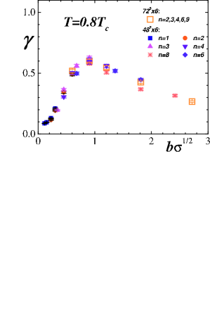
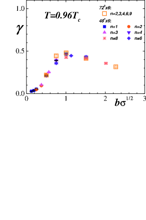
(a)	(b)

Figure 3: The same as in Figure 1 but for the coefficient $\gamma$ of the distribution (16).

we show the coupling constant $\gamma(b,T)$ as a function of the scale parameter, $b$, at temperatures $T=0.8\,T_{c}$ and $T=0.96\,T_{c}$. Again, as in the case of the parameter $f_{0}$, Figure 1, we observe the volume independence and the $b$–scaling of the results. In a small $b$–region we find that $\gamma\propto b^{\eta}$ with $\eta\sim 3$ for low temperatures, $T\sim 0.5T_{c}$, whereas $\eta\sim 2$ for $T\to T_{c}$. The data show a good $b$–scaling and also is independent of the volume similarly to the monopole action.

The numerical values of the parameter $A$ are shown in Figure 4. The parameter $A$ is independent of the lattice volume, indicating that in the thermodynamic limit the coefficient $\alpha$ in the Gaussian distribution (16) vanishes.

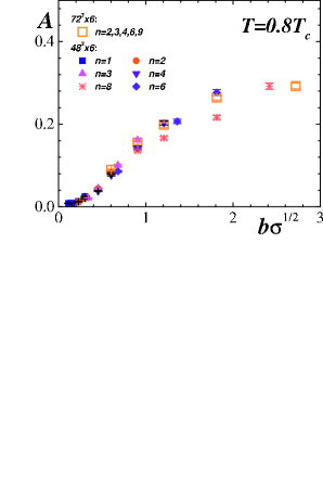
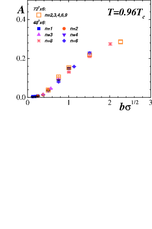
(a)	(b)

Figure 4: The same as in Figure 1 but for the ratio $A(b)$, Eq. (18).

Using Eq. (19) we calculate the monopole density corresponding to the infrared cluster. The density is shown in Figure 5.

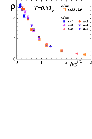
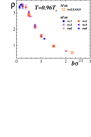
(a)	(b)

Figure 5: The same as in Figure 1 but for the monopole density $\rho$ corresponding to the infrared cluster, Eq. (19).

The density diminishes as the scale factor $b$ increases, while at small $b$ the density shows a plateau. As the temperature increases the density (at a fixed value of $b$) becomes smaller.

Note that the confining non–Abelian objects have a finite size (in physical units). These objects are identified as the Abelian monopoles in the Abelian gauge. The monopoles are detected using the Gauss theorem applied to the magnetic field coming outside the cube of the size $b^{3}$. The confining non–Abelian objects have a typical size which is associated with the size of the monopole core ref:rmon , $r_{mon}\approx 0.05$ fm. If $b<r_{mon}$ then the monopole cube is too small to detect the charge of much larger monopole and the monopole density – measured using the Gauss law – is vanishingly small. Indeed, one can see that the monopole density in Figure 5 has a tendency to diminish at smaller $b\sqrt{\sigma}\lesssim 0.1$.

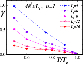
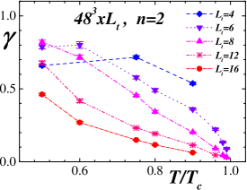
(a)	(b)
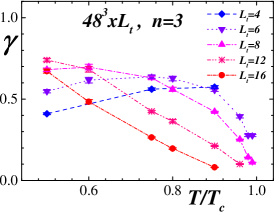
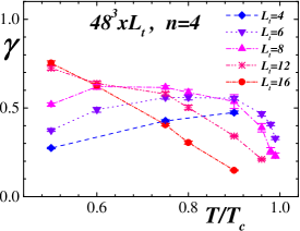
(c)	(d)

Figure 6: The coefficient $\gamma$ vs. temperature $T$ for various temporal extensions of the lattice and for various blacking factors $n$.

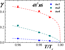
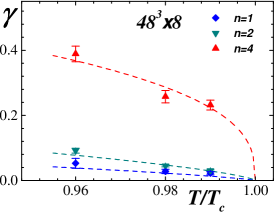
(a)	(b)

Figure 7: Examples of the fits of the $\gamma$ parameter as the function of the temperature.

At the critical temperature, $T=T_{c}$, the $4D$ IR monopole cluster disappears and we expect a similar behavior for the $3D$ projected IR cluster. This implies, that the parameter $\gamma(b,T)$ must become a (non-local) order parameter: it must vanish at the critical point. One can reach this conclusion by noticing that the parameter $\gamma(b,T)$ is proportional to the monopole density (19) (which vanishes at $T=T_{c}$), and that the factor $A$ is unlikely to be divergent at the critical temperature (what can also be deduced from Figures 4).

We show that the quantity $\gamma$ is indeed an order parameter in Figure 6(a) which depicts $\gamma$ for elementary ($n=1$) monopoles as a function of temperature for various temporal extensions of the lattice. The behavior of the $\gamma$-parameter in the vicinity of the phase transition point depends on the value of the temporal extension $L_{t}$. However, the value of the $\gamma$–parameter at the critical temperature, $\gamma(T\to T_{c})\to 0$, is universal with respect to $L_{t}$. Moreover, one can observe in Figures 6(b,c,d) – which correspond to the extensions $n=2,3,4$, respectively – that the $\gamma$-coefficient for the extended monopoles is also vanishing at $T=T_{c}$.

To characterize the critical behavior of the parameter $\gamma$ in the vicinity of the phase transition we have fitted this parameter by the function

$$\gamma^{\mathrm{fit}}(b,T)=C_{\gamma}\cdot\Bigl{(}1-\frac{T}{T_{c}}\Bigr{)}^{\delta}\,,\qquad T<T_{c}\,,$$ (20)

where $\delta$ and $C_{\gamma}$ are the fitting parameters. We performed the fits for various lattices $L_{s}^{3}\times L_{t}$ and extensions $n$. The results for the ”critical exponent” $\delta$ are shown in Table 1.

$\delta$
$\ n\$	$\ 48^{3}\times 6\$	$\ 48^{3}\times 8\$	$\ 72^{3}\times 8\$
1	0.64(15)	0.76(2)	–
2	0.62(8)	0.70(16)	0.48(3)
3	0.34(6)	0.55(7)	0.30(2)
4	0.22(2)	0.36(6)	0.18(3)
6	0.11(2)	0.20(2)	–

Table 1: The ”critical exponents” $\delta$ – obtained with the help of the fit (20) – for various lattices $L_{s}^{3}\times L_{t}$ and extensions $n$.

From this table one notices that the quantity $\delta$ is not universal: it depends not only on the extension of the monopole blocking but also it also depends on the lattice volume. Moreover, the larger extension $n$ the steeper behavior of $\gamma$ in the vicinity of the phase transition is.

One should add a word of caution here. The fit results shown in Table 1 are crucially dependent of the $T/T_{c}=0.98,0.99$ points (as one can see from Figures 7(a),(b)), which are very close to the phase transition. Since the transition is of the second order then the finite–volume effects must be strong and the results of fits may quantitatively be incorrect (although the results presented in Figures 7(a),(b) must qualitatively be correct).

V Monopole entropy

Apart from the finite–volume effect, the distribution (16) has contributions from the energy and the entropy. As seen above, the action contribution is proportional to $e^{-f_{0}L}$. The entropy contribution is proportional to $\mu^{L}$ (with $\mu>0$) for sufficiently large monopole lengths, $L$. Thus, the entropy factor, $\mu$, is

$$\mu=\exp\{f_{0}+\gamma\}\,.$$ (21)

We determine the entropy using Eq. (21). The numerical results for the entropy factor $\mu(b,T)$ are shown in Figures 8 for various temperatures, lattice volumes and blocking factors.

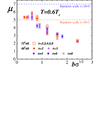
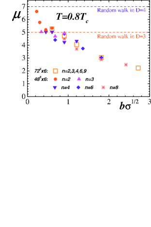
(a)	(b)
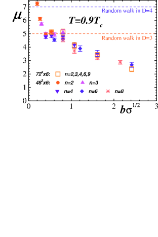
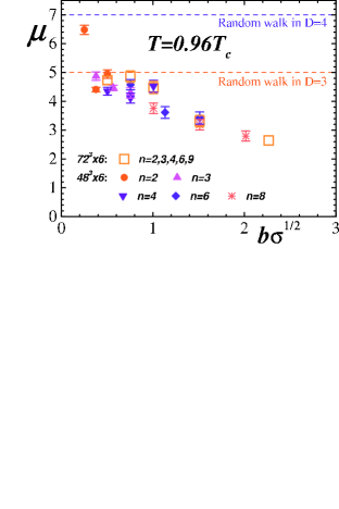
(c)	(d)
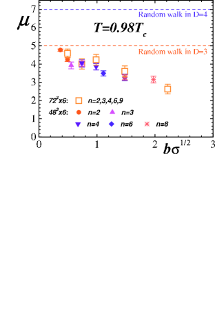
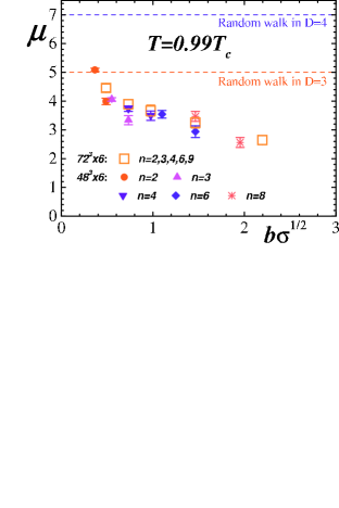
(e)	(f)

Figure 8: Entropy factor of the spatially projected monopole currents as the function of the scale $b$ at various temperatures.

One can see that the entropy factor $\mu$ scales as the function of $b$, as expected.

In order to understand the meaning of the data shown in Figure 8 we note that if the monopoles are randomly walking on a $3D$ hypercubic lattice then we should get a definite value for the entropy factor, $\mu=5$. This is because at each site there exist five choices for the monopole current to go further. One can see that far from the phase transition, $T\lesssim 0.96T_{c}$ the entropy factor $\mu$ indeed tends to the $\mu=5$ plateau at moderately small values of $b\sim 0.4\dots 1$. At yet smaller $b$ the entropy gets bigger than random walk value $\mu>5$ because in this region the inverse Monte-Carlo method with the truncated quadratic monopole action does not work well chernodub . Thus, the value of the constant $f_{0}$ – defined in Eq. (15) – can not be obtained correctly.

At large $b$ the entropy factor drops down with the increase of the factor $b$. This feature is independent of the temperature. In the zero temperature case IshiguroSuzuki the entropy factor $\mu$ approaches unity in the $b\to\infty$ limit. This feature is difficult to observe from our data since the information about the entropy at large values of the blocking size $b$ is not available.

VI Conclusion

The distributions of the spatially–projected infrared monopole currents of various blocking sizes, $n$ were studied on the lattices with different spacings, $a$, and volumes, $L_{s}^{3}\times L_{t}$. We find that the distributions can be described by a gaussian anzatz with a good accuracy. The anzatz contains two important terms: (i) the linear term, which contains information about the energy and entropy of the monopole currents; and (ii) the quadratic term, which appears due to finite–volume and which suppresses large infrared clusters. The linear term is independent of the lattice volume while the quadratic term is inversely proportional to the volume. Moreover, the linear term is a (non–local) order parameter for the deconfinement phase transition.

To get the entropy of the spatially–projected currents we studied the action of the monopoles belonging to the infrared monopole clusters of the spatially–projected currents using an inverse Monte-Carlo method. We show that the entropy factor has a plateau at sufficiently small values of $b$ and at $T\lesssim 0.96T_{c}$. A reason for the temperature restriction of our result is that our analysis may not be valid close to the second order phase transition point because of the increase of correlation lengthes at (and, consequently, because of strong finite-volume effects) $T\approx T_{c}$. At $b\gtrsim 1$ the entropy is a descending function of $b=na$, indicating that the effective degrees of freedom of the projected and blocked monopoles are getting smaller as the blocking scale $b$ increases. This effect is very similar to the zero temperature case, in which the monopole motion corresponds to the classical picture: the monopole with the large blocking size $b$ becomes a macroscopic object and the motion of such a monopole gets close to a straight line.

- (1) G. ’t Hooft, in High Energy Physics, ed. A. Zichichi, EPS International Conference, Palermo (1975); S. Mandelstam, Phys. Rept. 23, 245 (1976).
- (2) G. ’t Hooft, Nucl. Phys. B190, 455 (1981).
- (3) A. S. Kronfeld, M. L. Laursen, G. Schierholz and U. J. Wiese, Phys. Lett. B198, 516 (1987); A. S. Kronfeld, G. Schierholz, U. J. Wiese, Nucl. Phys. B293, 461 (1987).
- (4) K. Amemiya, H. Suganuma, Phys. Rev. D 60, 114509 (1999); V. G. Bornyakov, M. N. Chernodub, F. V. Gubarev, S. M. Morozov, M. I. Polikarpov, Phys. Lett. B 559, 214 (2003).
- (5) T. Suzuki, Nucl. Phys. Proc. Suppl. 30, 176 (1993); M. N. Chernodub, M. I. Polikarpov, in ”Confinement, duality, and nonperturbative aspects of QCD”, Ed. by P. van Baal, Plenum Press, p. 387, hep-th/9710205 (1997); R.W. Haymaker, Phys. Rept. 315, 153 (1999).
- (6) T. Suzuki and I. Yotsuyanagi, Phys. Rev. D42, 4257 (1990); G. S. Bali, V. Bornyakov, M. Müller-Preussker and K. Schilling, Phys. Rev. D54, 2863 (1996).
- (7) H. Shiba and T. Suzuki, Phys. Lett. B 333, 461 (1994);
- (8) H. Shiba, T. Suzuki, Phys. Lett. B351 519, (1995); N. Arasaki, S. Ejiri, S. i. Kitahara, Y. Matsubara and T. Suzuki, Phys. Lett. B395 275, (1997).
- (9) M.Chernodub, M.I.Polikarpov, A.I.Veselov, Phys. Lett. B399, 267 (1997); Nucl. Phys. Proc. Suppl. 49, 307 (1996).
- (10) T.L. Ivanenko, A.V. Pochinsky, M.I. Polikarpov, Phys. Lett. B252, 631 (1990).
- (11) S. Kitahara, Y. Matsubara, T. Suzuki, Progr. Theor. Phys. 93, 1 (1995).
- (12) A. Hart, M. Teper, Phys. Rev., B58, 014504 (1998). P.Y. Boyko, M.I. Polikarpov, V.I. Zakharov, Nucl.Phys.Proc.Suppl. 119, 724 (2003); M. N. Chernodub, V. I. Zakharov, Nucl. Phys. B669, 233 (2003); V. G. Bornyakov, P.Yu. Boyko, M.I. Polikarpov, V.I. Zakharov, Nucl.Phys. B672, 222 (2003).
- (13) M.N.Chernodub, K.Ishiguro, K.Kobayashi, T.Suzuki, Phys. Rev. D 69, 014509 (2004); K.Ishiguro, M.N.Chernodub, K.Kobayashi, T.Suzuki, Nucl. Phys. Proc. Suppl. 129, 659 (2004).
- (14) T. Suzuki, M. N. Chernodub and K. Ishiguro, Nucl. Phys. Proc. Suppl. 129, 760 (2004).
- (15) T. A. DeGrand, D. Toussaint, Phys. Rev. D22, 2478 (1980).
- (16) M. N. Chernodub, S. Fujimoto, S. Kato, M. Murata, M. I. Polikarpov, T. Suzuki, Phys. Rev. D 62, 094506 (2000); M. N. Chernodub, S. Kato, N. Nakamura, M. I. Polikarpov, T. Suzuki, “Various representations of infrared effective lattice SU(2) gluodynamics”, hep-lat/9902013.
- (17) V. G. Bornyakov, M. N. Chernodub, F. V. Gubarev, M. I. Polikarpov, T. Suzuki, A. I. Veselov and V. I. Zakharov, Phys. Lett. B 537, 291 (2002).