$I=2$ Pion Scattering Length from Two-Pion Wave Functions

Abstract

We calculate the two-pion wave function in the ground state of the $I=2$ $S$-wave system and find the interaction range between two pions, which allows us to examine the validity of the necessary condition for the finite-volume method for the scattering length proposed by Lüscher. We work in the quenched approximation employing a renormalization group improved gauge action for gluons and an improved Wilson action for quarks at $1/a=1.207(12)\ {\rm GeV}$ on $16^{3}\times 80$, $20^{3}\times 80$ and $24^{3}\times 80$ lattices. We conclude that the necessary condition is satisfied within the statistical errors for the lattice sizes $L\geq 24$ ($3.92\ {\rm fm}$) when the quark mass is in the range that corresponds to $m_{\pi}^{2}=0.273-0.736\ {\rm GeV}^{2}$. We obtain the scattering length with a smaller statistical error from the wave function than from the two-pion time correlator.

I Introduction

Calculations of the scattering length and the phase shift represent an important step for expanding our understanding of the strong interaction based on lattice QCD to dynamical aspects of hadrons. For the simplest case of the two-pion system in the $I=2$ $S$-wave system, the scattering length has been calculated in SGK:a0 ; GPS:a0 ; KFMOU:a0 ; AJ:a0 ; Juge:a0 ; JLQCD:a0 ; LZCM:a0 ; DMML:a0 ; BGR:a0 and the pioneering study of the phase shift was made by Fiebig et al. Fiebig:phsh using the two-pion effective potential. We presented a direct calculation of the phase shift without recourse to the effective potential in quenched CP-PACS:phsh and full QCD CP-PACS:phsh_full . Kim reported on preliminary results of the phase shift on $G$- and $H$-periodic boundary lattices Kim:phsh .

The calculation of the scattering length and the phase shift usually employs the finite-volume method of Lüscher, in which the scattering phase shift is related to the energy eigenvalue on a finite volume Luscher_one:formula ; Luscher_LH:formula ; LuscherWolf:formula ; Luscher_two:formula . In previous application of the formula the energy eigenvalues were calculated from the asymptotic time behavior of the two-pion time correlator.

The derivation of Lüscher’s formula assumes the condition $R<L/2$ for the two-pion interaction range $R$ and the lattice size $L$, so that the boundary condition does not distort the shape of the two-pion interaction. In the studies to date, however, calculations were carried out without verifying this necessary condition, but simply employing a few lattices having different sizes and extrapolating to the infinite volume limit assuming simple functions, such as an inverse power of the lattice extent, for finite volume corrections. In the absence of theoretical justification, however, such assumptions would cause ambiguities and it is important to examine the validity of the condition in lattice simulations for reliable results.

In this work we restrict ourselves to the ground state of the $I=2$ $S$-wave two-pion system and calculate the two-pion wave function. We investigate the two-pion interaction range and the validity of the necessary condition for Lüscher’s formula. We attempt to extract the scattering length directly from the wave function and compare it with the more conventional result from the two-pion time correlator.

We refer to the work for two-dimensional statistical models in Wisz:stat . For the two-pion system of QCD a similar idea was discussed in LMST:kpp . We also quote Yamazaki who presented preliminary results for the wave function for the four-dimensional Ising model and the scattering phase shift therefrom Yamazalo:ISppwf .

This paper is organized as follows. In Sec. II we give a brief review of the derivation of Lüscher’s formula Luscher_two:formula with emphasis on the role of the condition $R<L/2$. The calculational method of the wave function and the simulation parameters are given in Sec. III. In Sec. IV.1 we present the wave function and estimate the two-pion interaction range for a $24^{3}$ lattice. In Sec. IV.2 we calculate the scattering length from the wave function and compare it with that from the two-pion time correlator. Our investigations on $20^{3}$ and $16^{3}$ lattices are given in Sec. IV.3, where finite volume effects on the scattering length are examined by comparing three lattice volumes. Our conclusions are given in Sec. V. Preliminary reports of the present work were presented in IY:ppwf .

II Lüscher’s formula

We briefly review the derivation of Lüscher’s formula, with emphasis on the role of the condition for the two-pion interaction range. The formula Luscher_one:formula ; Luscher_LH:formula was rederived using an effective Schrödinger equation for the two-dimensional scalar filed theory in LuscherWolf:formula , and for the four-dimensional case in Luscher_two:formula which is discussed here. Another approach based on the Bethe-Salpeter wave function in quantum field theory LMST:kpp is discussed in Appendix. A.

The static two-pion wave function $\phi(\vec{x};k)$ with the energy eigenvalue $E=2\sqrt{k^{2}+m_{\pi}^{2}}$ in the center of mass system on a finite periodic box of volume $L^{3}$ satisfies the effective Schrödinger equation Luscher_one:formula ; LuscherWolf:formula :

$$(\triangle+k^{2})\phi(\vec{x};k)=\int{\rm d}^{3}y\ U_{k}(\vec{x},\vec{y})\phi(\vec{y};k)\ ,$$ (1)

where $\vec{x}$ and $\vec{y}$ are the relative coordinate of the two pions. $U_{k}(\vec{x},\vec{y})$ is the Fourier transform of the modified Bethe-Salpeter kernel for the two-pion interaction on the finite volume Luscher_one:formula , and is related to the off-shell two-pion scattering amplitude (see Appendix A). It is generally non-local and depends on the two-pion energy. It should be noticed that $k^{2}$ in (1) is not a square of a 3-dimensional momentum vector but defined from the energy by $k^{2}=E^{2}/4-m_{\pi}^{2}$. It may take a negative value in some cases. We call $k$ “momentum” for simplicity in this paper, however.

In the derivation of Lüscher’s formula it is assumed that the two-pion interaction range is smaller than one half the lattice extent, i.e. there exists the distance $R<L/2$, where the wave function satisfies the Helmholtz equation :

$$(\triangle+k^{2})\phi(\vec{x};k)=0\quad\mbox{ for $\vec{x}\in V_{R}$ }\ ,$$ (2)

with

$$V_{R}=\{\ \vec{x}\ |\ |\vec{x}+\vec{n}L|>R\ ,\ \vec{n}\in{\bf Z}^{3}\ \}\ .$$ (3)

Next we consider solutions of (2). In general $k^{2}L^{2}/(2\pi)^{2}$ can be integer or non-integer. The former case is called “singular-value solutions” in Luscher_two:formula (see also LMST:kpp ). The appearance of these solutions is not generic. It occurs only for some specific lattice volumes or particular cases of the two-pion interaction. For the two-pion ground state there is an important singular-value solution that has $k^{2}=0$, which, however, exists only on specific lattice volumes or for the vanishing scattering length. If this solution appears in numerical simulations, the two-pion time correlator should behave as

$$\frac{\langle 0|\pi(t)\pi(t)\pi(0)\pi(0)|0\rangle}{\langle 0|\pi(t)\pi(0)|0\rangle^{2}}\sim\mbox{ const.}\ ,$$ (4)

for a large $t$. However, such a time behavior has not been observed in previous studies or in our numerical simulations. Thus such a case hardly occurs for the ground state. The formula for the singular-value solutions was derived in Ref. Luscher_two:formula , but we consider only non-integer value solutions in this paper.

General solutions of the Helmholtz equation (2) can be written by

$$\phi(\vec{x};k)=\sum_{l=0}^{\infty}\sum_{m=-l}^{l}\ v_{lm}(k)\cdot G_{lm}(\vec{x};k)\ ,$$ (5)

with $v_{lm}(k)$. $G_{lm}(\vec{x};k)$ is given from the periodic Green function :

$$G(\vec{x};k)=\frac{1}{L^{3}}\sum_{\vec{p}\in\Gamma}\ \frac{1}{p^{2}-k^{2}}\ {\rm e}^{i\vec{p}\cdot\vec{x}}\ ,\quad\Gamma=\bigl{\{}\ \vec{p}\ |\ \vec{p}=\vec{n}\frac{2\pi}{L}\ ,\ \vec{n}\in{\bf Z}^{3}\bigr{\}}\ ,$$ (6)

as

$$G_{lm}(\vec{x};k)=\sqrt{4\pi}{\cal Y}_{lm}(\nabla)G(\vec{x};k)\ ,$$ (7)

where ${\cal Y}_{lm}(\vec{x})$ is a polynomial related to the spherical harmonics through ${\cal Y}_{lm}(\vec{x})=x^{l}\cdot Y_{lm}(\Omega_{x})$ with $\Omega_{x}$ the spherical coordinate for $\vec{x}$ and $x=|\vec{x}|$. The convention of $Y_{lm}(\Omega)$ is that of MESSIAH:book , as is adopted in Luscher_two:formula . It then follows that $G_{00}(\vec{x};k)=G(\vec{x};k)$.

In general we can expand the solution of the Helmholtz equation in terms of the spherical Bessel $j_{l}(kx)$ and Neumann functions $n_{l}(kx)$ for $R<x<L/2$ as

$$\phi(\vec{x};k)=\sum_{l=0}^{\infty}\sum_{m=-l}^{l}\sqrt{4\pi}Y_{lm}(\Omega_{x})\biggl{(}\alpha_{l}(k)\cdot j_{l}(kx)+\beta_{l}(k)\cdot n_{l}(kx)\biggr{)}\ ,$$ (8)

where the conventions of $j_{l}(x)$ and $n_{l}(x)$ agree with those in MESSIAH:book and Luscher_two:formula . The expansion coefficients $\alpha_{l}(k)$ and $\beta_{l}(k)$ yield the scattering phase shift in the infinite volume as $\tan\delta_{l}(k)=\beta_{l}(k)/\alpha_{l}(k)$. In particular, for the ground state the momentum $k^{2}$ is very small and the $S$-wave scattering length $a_{0}$ is given by $\tan\delta_{0}(k)=\beta_{0}(k)/\alpha_{0}(k)=a_{0}k+{\rm O}(k^{3})$.

For the wave function (5), $\beta_{l}(k)$ and $\alpha_{l}(k)$ are geometrically related, because they can be expressed in terms of the expansion coefficients for $G_{lm}(\vec{x};k)$. The expansion of $G(\vec{x};k)$ is given by

$$G(\vec{x};k)=\frac{k}{4\pi}n_{0}(kx)+\sum_{l=0}^{\infty}\sum_{m=-l}^{m=l}\sqrt{4\pi}Y_{lm}(\Omega_{x})g_{lm}(k)j_{l}(kx)\ ,$$ (9)

where

$$g_{lm}(k)=\frac{1}{L^{3}}\sum_{\vec{p}\in\Gamma}\frac{(ip/k)^{l}}{p^{2}-k^{2}}\sqrt{4\pi}Y_{lm}(\Omega_{p})\ ,\quad\Gamma=\bigl{\{}\ \vec{p}\ |\ \vec{p}=\vec{n}\frac{2\pi}{L}\ ,\ \vec{n}\in{\bf Z}^{3}\bigr{\}}$$ (10)

with spherical coordinate $\Omega_{p}$ for $\vec{p}$. (The function $g_{lm}(k)$ differs from $g_{lm}$ in (3.31) of Ref. Luscher_two:formula only by the normalization as $g_{lm}(k)=1/\sqrt{4\pi}\cdot g_{lm}$). The explicit expansion for $G_{lm}(\vec{x};k)$ with general $l$ and $m$ is not needed. Note that the indices $l$ and $m$ are not labels of the angular momentum, nor $G_{lm}(\vec{x};k)$ is the eigenstate of the angular momentum labeled by $l$ and $m$. Actually it includes $Y_{l^{\prime}m^{\prime}}(\Omega_{x})$ with $l^{\prime}\not=l$ and $m^{\prime}\not=m$. Also note that $G_{lm}(\vec{x};k)$ contains $j_{l^{\prime}}(kx)$ for a range of $l^{\prime}$ and $n_{l^{\prime}}(kx)$ with only $l^{\prime}=l$. These are easily known from (7) and (9).

In this work we consider only wave functions in the ${\bf A_{1}^{+}}$ representation of the cubic group, which equals $S$-wave up to angular momenta $l\geq 4$. The wave function for $\vec{x}\in V_{R}$ can be expressed as

$$\phi(\vec{x};k)=v_{00}(k)\cdot G(\vec{x};k)+v_{40}(k)\cdot\frac{1}{48}\sum_{{\bf R}}G_{40}({\bf R}[\vec{x}];k)+\cdots\ ,$$ (11)

where a vector operation ${\bf R}$ represents an element of the cubic group which has 48 elements. The terms with $l\geq 6$ are neglected, and the $l=4$ terms with $m\neq 0$ do not appear since they either vanish (for $|m|\not=4$) or reduce to $G_{40}(\vec{x};k)$ (for $|m|=4$). If the scattering phase shift $\delta_{l}(k)$ with $l\geq 4$ is negligible in the energy range under consideration, $\beta_{l}(k)\sim 0$ for $l\geq 4$ in (8). This means that $v_{40}(k)\sim 0$ in (11), and thus

$$\phi(\vec{x};k)\sim v_{00}(k)\cdot G(\vec{x};k)\ ,$$ (12)

because $G_{lm}(\vec{x};k)$ contains $n_{l}(kx)$. This expectation is supported for the ground state by our numerical simulations.

Finally we obtain Lüscher’s formula between the $S$-wave scattering phase shift and the allowed value of $k^{2}$ by comparing the coefficients of $j_{0}(kx)$ and $n_{0}(kx)$ in (9),

$$\frac{1}{\tan\delta_{0}(k)}=\frac{\alpha_{0}(k)}{\beta_{0}(k)}=\frac{g_{00}(k)}{k/(4\pi)}=\frac{4\pi}{k}\cdot\frac{1}{L^{3}}\sum_{\vec{p}\in\Gamma}\frac{1}{p^{2}-k^{2}}\ ,$$ (13)

where the region $\Gamma$ is defined by (10) and (12) is assumed.

We remark that contaminations from inelastic scattering are likely negligible for the ground state, although they may become significant for momentum excitation states, whose energies are close to or above the threshold of inelastic scattering, $E\sim 4m_{\pi}$.

III Method of calculations

III.1 Calculation of the wave function

Our definition of the two-pion wave function is

$$\phi(\vec{x};k)=\langle 0|\ \Omega(\vec{x},t)\ |\pi^{+}\pi^{+};k\rangle\cdot{\rm e}^{2E_{k}t}\ ,$$ (14)

where $|\pi^{+}\pi^{+};k\rangle$ is the ground state with energy $2E_{k}=2\sqrt{m_{\pi}^{2}+k^{2}}$. A factor $\exp(2E_{k}t)$ is introduced to compensate the $t$ dependence. The operator $\Omega(\vec{x},t)$ is an interpolating field for the two-pion, which is defined by

$$\Omega(\vec{x},t)=\frac{1}{48}\sum_{{\bf R}}\frac{1}{L^{3}}\sum_{\vec{X}}\ \pi^{+}({\bf R}[\vec{x}]+\vec{X},t)\ \pi^{+}(\vec{X},t)\ ,$$ (15)

where $\pi^{+}(\vec{x},t)=\bar{u}(\vec{x},t)\gamma_{5}d(\vec{x},t)$ is an interpolating operator for $\pi^{+}$ at $(\vec{x},t)$ and a vector operation ${\bf R}$ represents an element of the cubic group which has 48 elements. The summation over ${\bf R}$ and $\vec{X}$ projects out the ${\bf A_{1}^{+}}$ sector of the cubic group and the zero total momentum state. The wave function in (14) is the Bethe-Salpeter wave function projected to the ${\bf A_{1}^{+}}$ sector. It has the same properties as those of the wave function in Sec. II and we can derive Lüscher’s formula from it. Details are discussed in Appendix A. The wave functions at all positions $\vec{x}$ are not independent. The number of independent position vectors is $N(N+1)(N+2)/6$ with $N=L/2+1$ owing to the periodic boundary condition $\phi(\vec{x};k)=\phi(\vec{x}+\vec{n}L;k)$ with $\vec{n}\in{\bf Z}^{3}$ and the invariance under the cubic group $\phi(\vec{x};k)=\phi({\bf R}[\vec{x}];k)$.

In order to calculate the wave function we construct the correlator :

$$F_{\pi\pi}(\vec{x},t;t_{0},t_{0}+1)=\langle 0|\ \Omega(\vec{x},t)\ W(t_{0})\ W(t_{0}+1)\ |0\rangle\ ,$$ (16)

where $W(t)$ is a wall source at time $t$ defined by

$$W(t)=\frac{1}{L^{3}}\sum_{\vec{x}}\frac{1}{L^{3}}\sum_{\vec{y}}\bar{d}(\vec{x},t)\gamma_{5}u(\vec{y},t)\ ,$$ (17)

which is used on configurations fixed to the Coulomb gauge. The two wall sources are placed at different time slices $t_{0}$ and $t_{0}+1$ to avoid contaminations from Fierz-rearranged terms KFMOU:a0 . Neglecting contributions from the momentum excitation states in the large $t$ region, we obtain the wave function at the time slice $t$ as

$$\phi(\vec{x};k)=\frac{F_{\pi\pi}(\vec{x},t;t_{0},t_{0}+1)}{F_{\pi\pi}(\vec{x}_{0},t;t_{0},t_{0}+1)}\ ,$$ (18)

up to the overall constant, where $\vec{x}_{0}$ is the reference position.

We try to extract the energy eigenvalue of the two-pion and the scattering length from the wave function $\phi(\vec{x};k)$, but, for comparison, we also estimate them from the two-pion time correlator :

$$F_{\pi\pi}(t;t_{0},t_{0}+1)=\frac{1}{L^{3}}\sum_{\vec{x}}F_{\pi\pi}(\vec{x},t;t_{0},t_{0}+1)\ .$$ (19)

The single pion time correlator computed with the aid of the wall source,

$$F_{\pi}(t;t_{0})=\frac{1}{L^{3}}\sum_{\vec{x}}\langle 0|\pi^{+}(\vec{x},t)W(t_{0})|0\rangle\ ,$$ (20)

is used to construct the normalized two-pion correlator :

$$R(t)=\frac{F_{\pi\pi}(t;t_{0},t_{0}+1)}{F_{\pi}(t;t_{0})F_{\pi}(t,t_{0}+1)}\ .$$ (21)

In the absence of the singular-value solution that belongs to $k^{2}=0$, this behaves for a large $t$ as

$$R(t)=C\cdot{\rm e}^{-\Delta W\cdot(t-t_{0})}\ ,$$ (22)

where $C$ is a constant and

$$\Delta W=2E_{k}-2m_{\pi}=2\sqrt{m_{\pi}^{2}+k^{2}}-2m_{\pi}$$ (23)

is the energy shift due to the two-pion interaction on the finite volume. The momentum $k^{2}$ is calculated from $\Delta W$, and it can be used to estimate the scattering length via Lüscher’s formula.

III.2 Simulation parameters

Our simulation is carried out in quenched lattice QCD employing a renormalization group improved gauge action for gluons,

$$S_{G}=\frac{\beta}{6}\sum_{x}\biggl{(}C_{0}\sum_{\mu<\nu}W_{\mu\nu}^{1\times 1}(x)+C_{1}\sum_{\mu,\nu}W_{\mu\nu}^{1\times 2}(x)\biggr{)}\ .$$ (24)

The coefficient $C_{1}=-0.331$ of the $1\times 2$ Wilson loop $W_{\mu\nu}^{1\times 2}(x)$ is fixed by a renormalization group analysis RG-gauge:IW , and $C_{0}=1-8C_{1}=3.648$ of the $1\times 1$ Wilson loop $W_{\mu\nu}^{1\times 1}(x)$ by the normalization condition, which defines the bare coupling $\beta=6/g^{2}$. Our calculation is carried out at $\beta=2.334$. Gluon configurations are generated with the $5$-hit heat-bath algorithm and the over-relaxation algorithm mixed in the ratio of $1:4$. The combination is called a sweep and physical quantities are measured every 200 sweeps.

We use an improved Wilson action for the quarks SWW:SW with the clover coefficient $C_{SW}$ being the mean-field improved choice defined by

$$C_{SW}=(\overline{W}_{\mu\nu}^{1\times 1})^{-3/4}=(1-0.8412/\beta)^{-3/4}=1.398\ ,$$ (25)

where $\overline{W}_{\mu\nu}^{1\times 1}$ is the value in one-loop perturbation theory RG-gauge:IW . Quark propagators are solved with the Dirichlet boundary condition imposed in the time direction for gauge configurations fixed to the Coulomb gauge. The wall source defined by (17) is set at $t_{0}=12$ which is sufficient to avoid effects from the temporal boundary.

The lattice cutoff was estimated as $1/a=1.207(12)\ {\rm GeV}$ ($a=0.1632(16)\ {\rm fm}$) from $m_{\rho}$ CP-PACS:LHM . The lattice sizes (the numbers of configurations in parentheses) are $16^{3}\times 80$ $(1200)$, $20^{3}\times 80$ $(1000)$ and $24^{3}\times 80$ $(506)$, which correspond to the lattice extent $2.61$, $3.26$ and $3.92\ {\rm fm}$ in physical units. Five quark masses are chosen to give $m_{\pi}^{2}=$ $0.273$, $0.351$, $0.444$, $0.588$ and $0.736\ {\rm GeV}^{2}$. The numbers of positions that give independent wave functions are $165$, $286$ and $455$ for $L=16$, $20$ and $24$.

IV Results

IV.1 Wave functions

The two-pion wave function calculated on the $24^{3}$ lattice is exemplified in Fig. 1 on the $(t,z)=(52,0)$ plane for $m_{\pi}^{2}=0.273\ {\rm GeV}^{2}$, with the reference position in (18) fixed at $\vec{x}_{0}=(7,5,2)$ ($x_{0}=|\vec{x}_{0}|=8.832$). The statistical errors are negligible in the scale of the figure.

The same wave function is shown in Fig. 2 as a function of $x=|\vec{x}|$ for independent data points. The branching of the curve seen in the figure indicates that the wave function does not represent a pure $S$-wave. This can be understood by the consideration in what follows. Let $f(x)$ be a function depending only on $x=|\vec{x}|$ for $\vec{x}=[-L/2,L/2]^{3}$. The first derivative is given by

$$\nabla f(x)=\frac{\vec{x}}{x}\frac{\rm d}{{\rm d}x}f(x)\ .$$ (26)

Thus $f(x)$ satisfies the boundary condition only when ${\rm d}f(x)/{\rm d}x=0$ at the boundary where at least one component of the vector $\vec{x}$ takes $\pm L/2$. This also means ${\rm d}f(x)/{\rm d}x=0$ for $x\geq L/2$ from symmetry under the cubic group. The wave function for the scattering system generally does not satisfy this. Hence it cannot be a pure $S$-wave function, but receives contributions from the states with angular momenta $l>0$. We expect that the wave function that belongs to the ${\bf A_{1}^{+}}$ representation contains $j_{l}(kx)$ with $l\geq 4$, but not $n_{l}(kx)$ with $l\geq 4$, because $\delta_{l}(k)$ is small for $l\geq 4$ for the two-pion ground state. This is supported by our results as shown latter.

We now consider the two-pion interaction from the ratio :

$$V(\vec{x};k)=\frac{\triangle\phi(\vec{x};k)}{\phi(\vec{x};k)}\ .$$ (27)

Here we adopt the naive numerical Laplacian on the lattice,

$$\triangle f(\vec{x})=\sum_{\mu}\bigl{[}f(\vec{x}+\hat{\mu})-f(\vec{x}-\hat{\mu})+2f(\vec{x})\bigr{]}\ ,$$ (28)

since $k^{2}$ is very small and the choice of the numerical Laplacian is not important for a large $x$. Away from the two-pion interaction range, i.e. $x>R$, we expect that $V(\vec{x};k)$ is independent of $\vec{x}$ and equals to $-k^{2}$. In Fig. 3 $V(\vec{x};k)$ is plotted for the same parameters as for Fig. 1. The statistical errors are again negligible. We find a very clear signal and $V(\vec{x};k)$ seems to be constant for $x>8$. We observe a strong repulsive interaction at the origin consistent with the negative scattering length of the $I=2$ two-pion system.

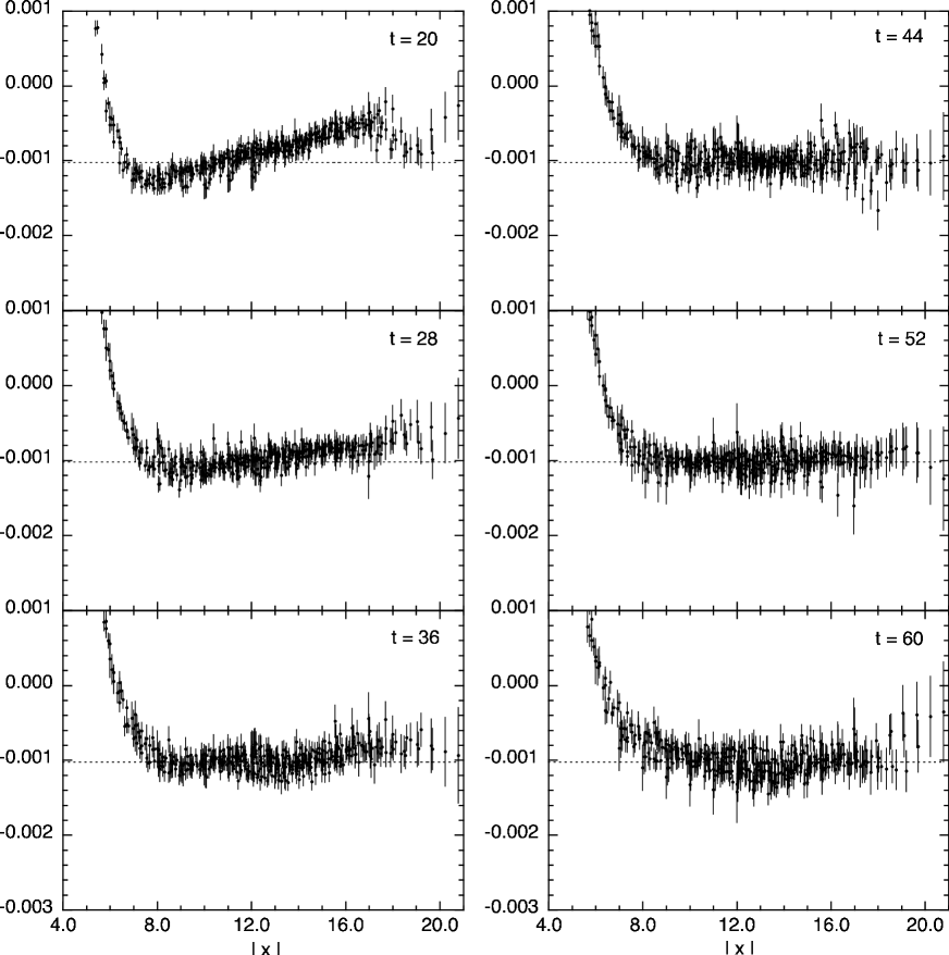
Figure 4: Time dependence of $V(\vec{x};k)$ in unit of $1/a^{2}$ on $24^{3}$ lattice for $m_{\pi}^{2}=0.273\ {\rm GeV}^{2}$. Horizontal axis is $x=|\vec{x}|$. We plot a line at $-k^{2}$ estimated from the two-pion time correlator.

The time dependence is shown in Fig. 4 for the same parameters, where the abscissa is $x=|\vec{x}|$ and only independent data are plotted. We draw a line of $-k^{2}$ estimated from $\Delta W$ of (22) using the normalized two-pion time correlator $R(t)$. We see that $V(\vec{x};k)$ approaches a value consistent with $-k^{2}$ for a large $x$. $V(\vec{x};k)$ depends only on $x$ and does not depend on $t$ in so far as $t\geq 44$. We also confirm that the wave function $\phi(\vec{x};k)$ does not vary when $t$ is varied for $t\geq 44$.

We now consider the two-pion interaction range $R$. In quantum field theory the wave function does not strictly satisfy the Helmholtz equation (2) even for the large $x$ region in a large volume lattice. Hence, with $k^{2}$ obtained from the asymptotic time behavior of the two-pion time correlator, $V(\vec{x};k)+k^{2}$ shows a small tail at a large $x$.

We may take the wave function as satisfying the Helmholtz equation, if $V(\vec{x};k)+k^{2}$ is sufficiently small compared with $k^{2}$. In the present work we take an operational definition for the range $R$ as the scale, where

$$U(\vec{x};k)=\frac{V(\vec{x};k)+k^{2}}{k^{2}}=\frac{(\triangle+k^{2})\phi(\vec{x};k)}{k^{2}\phi(\vec{x};k)}$$ (29)

gets small enough so that it is buried into the statistical error, with the expectation that the systematic error for the scattering length from the interaction of tails of the wave function becomes smaller than statistical errors in the resulting scattering length with this definition. 

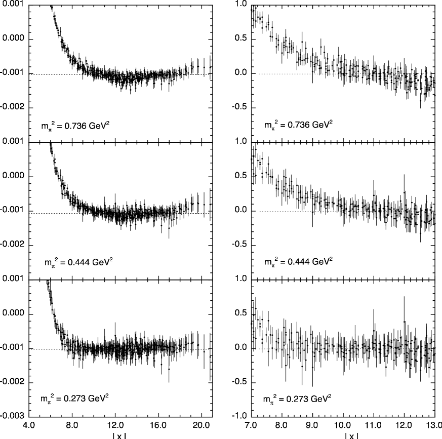
Figure 5: $V(\vec{x};k)$ in unit of $1/a^{2}$ (left side) and $U(\vec{x};k)$ (right side) on $24^{3}$ lattice at $t=52$ for several quark masses. Horizontal axis is $x=|\vec{x}|$. We plot a line at $-k^{2}$ obtained from the two-pion time correlator in left side of figures.

The function $U(\vec{x};k)$ is displayed in Fig. 5 at $t=52$, together with $V(\vec{x};k)$ defined by (27), for which the line of $-k^{2}$ estimated from the two-pion time correlator is also drawn. These figures show that $V(\vec{x};k)\sim-k^{2}$ and $U(\vec{x};k)\sim 0$ for $x>R$ within the statistical error for all quark masses. We find $R\sim 10$ ($1.6\ {\rm fm}$) for the heaviest quark mass, $m_{\pi}^{2}=0.736\ {\rm GeV}^{2}$. This stands for the largest $R$ we obtained. This result signifies that the necessary condition for Lüscher’s formula (2) is satisfied on the $24^{3}$ lattice for all our quark masses $m_{\pi}^{2}=0.273-0.736\ {\rm GeV}^{2}$ with the current statistics of simulations.

IV.2 Scattering lengths

We may estimate the scattering length from the wave function with two alternative methods :

1. We extract $k^{2}$ by fitting the asymptotic value of $V(\vec{x};k)$ to a constant and obtain the scattering length by substituting $k^{2}$ into (13). The resulting $k^{2}$ and the scattering length are given in Table 1 in the column labeled with “from $V$”. We choose $t=52$ and the fitting range $x_{m}\leq x\leq\sqrt{3}L/2$ (maximum value of $x$ for $L^{3}$ lattice). The energy shift $\Delta W$ is calculated from $k^{2}$ using (23).

2. $k^{2}$ is obtained by fitting the wave function $\phi(\vec{x};k)$ with periodic Green function $G(\vec{x};k)$ defined by (6), taking $k^{2}$ and an overall constant as free parameters. An example of fitting is illustrated in Fig. 2 at $t=52$ for $m_{\pi}^{2}=0.273\ {\rm GeV}^{2}$, where the values from fits are shown with cross symbols. The fitting range is the same as that for method 1. The method for numerical evaluation of $G(\vec{x};k)$ is discussed in Appendix B. The fit works well, meaning that the contributions of $G_{lm}(\vec{x};k)$ and $\delta_{l}(k)$ with $l\geq 4$ are negligible as expected. This point is confirmed by fitting with the function including $G_{40}(\vec{x};k)$. The results are given in Table 1 (labeled “from $\phi$”).

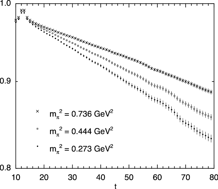
Figure 6: Normalized two-pion correlator $R(t)$ on $24^{3}$ lattice for $m_{\pi}^{2}=0.273$ (lightest), $0.44$ and $0.736\ {\rm GeV}^{2}$ (heaviest). Scale of vertical axis is log-scale.

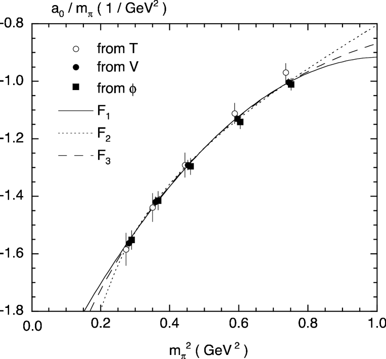
Figure 8: Pion scattering length $a_{0}/m_{\pi}\ (1/{\rm GeV}^{2})$ on $24^{3}$ lattice obtained from the two-pion time correlator (“from $T$”), the constant fit of $V(\vec{x};k)$ (“from $V$”) and the fitting the wave function (“from $\phi$”). Results of the chiral extrapolation of $a_{0}/m_{\pi}$ obtained from $V(\vec{x};k)$ (“from $V$”) with the three fitting functions are also plotted lines.

We compare the scattering lengths obtained from the wave function with those from the conventional method of using the two-pion time correlator. We plot the normalized two-pion correlator $R(t)$ of (21) in Fig. 6, which shows a clear signal that decreases exponentially in $t$. This means the absence of the singular-value solution for this volume, or otherwise $R(t)$ should approach some constant. The effective masses for $R(t)$ presented in Fig. 7 show the plateau over $t\sim 22-70$. Rows indicated with the label “from T” in Table 1 present the values of $\Delta W$ obtained by a single exponential fitting for $t=24-68$, $k^{2}$ estimated from $\Delta W$, and the scattering length from Lüscher’s formula (13), using $k^{2}$ thus estimated and $g_{00}(k)$ calculated by the numerical method discussed in CP-PACS:phsh . We compare the scattering length obtained from three methods in Fig. 8. The three methods give consistent results within statistical errors. We observe that the statistical errors for those from our new methods (“from $V$” and “from $\phi$”) are significantly smaller than those from the two-pion time correlator (“from $T$”). This feature was experienced in the two-dimensional statistical models Wisz:stat . Our analysis so far is made at $t=52$, but we checked that the results are independent of the choice of $t$ in so far as $t\geq 48$.

When one wants to obtain scattering lengths for the physical pion mass, there is yet an important problem of the chiral extrapolation. In Fig. 8 we carry out the chiral extrapolation of $a_{0}/m_{\pi}$ using the data from method 1 (i.e. “from $V$”) by assuming three fitting forms :

$$F_{1}(m_{\pi}^{2}) = A_{1}+B_{1}\cdot m_{\pi}^{2}+C_{1}\cdot m_{\pi}^{4}$$ (30)

$$F_{2}(m_{\pi}^{2}) = A_{2}+B_{2}/m_{\pi}^{2}+C_{2}\cdot m_{\pi}^{2}$$ (31)

$$F_{3}(m_{\pi}^{2}) = A_{3}\biggl{(}1+B_{3}\cdot m_{\pi}^{2}\cdot\log(m_{\pi}^{2}/C_{3})\biggr{)}\ \ .$$ (32)

The form of $F_{2}(m_{\pi}^{2})$ is motivated from chiral symmetry breaking of the Wilson fermion and quenching effects, as suggested from quenched chiral perturbation theory Bernard-Golterman:QCHPT ; Colangelo-Pallante:QCHPT . $F_{3}(m_{\pi}^{2})$ is the form predicted by chiral perturbation theory (CHPT) for full QCD in the one loop order. $F_{1}(m_{\pi}^{2})$ is a simple polynomial. We see that the three functions fit the data equally well and we cannot distinguish among them. The chiral limit of $a_{0}/m_{\pi}(=A_{j})$, however, depends sizably on the choice of the fitting forms :

$$a_{0}/m_{\pi}\ (1/{\rm GeV}^{2}) =\ -2.117(83) F_{1}(m_{\pi}^{2})$$ from (33)

$$=\ -1.29(15)\ F_{2}(m_{\pi}^{2})$$ from (34)

$$=\ -2.39(16)\ \mbox{ from $F_{3}(m_{\pi}^{2})$ }\ \ .$$ (35)

We cannot reduce this large systematic errors arising from the choice of fitting forms, unless simulations are made close to the physical pion mass or the fitting form is theoretically constrained. We add that the prediction from CHPT is $a_{0}/m_{\pi}=-2.265(51)\ (1/{\rm GeV}^{2})$ CHPT_a0_cont:CHPT .

IV.3 Results on small lattices

We carry out the same analysis for $20^{3}$ and $16^{3}$ lattices to study the dependence on the finite lattice size, with the numerical results presented in Tables 2 and 3.

Our analysis on the $24^{3}$ lattice shows that the two-pion interaction range is at most $R\sim 10$ ($1.6\ {\rm fm}$) which happens for the heaviest quark mass, $m_{\pi}^{2}=0.736\ {\rm GeV}^{2}$, so that Lüscher’s formula (13) is safely applied for the $24^{3}$ lattice for all our quark masses with the present statistical accuracy. This appears to indicate that $20^{3}$ is needed and $16^{3}$ may be too small. This is not necessarily true, however, since $R$ depends on the quark mass and the momentum $k^{2}$ which strongly depends on the lattice volume, as is seen by comparing the relevant entries in the three tables.

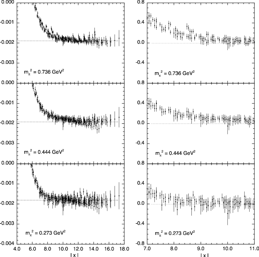
Figure 9: $V(\vec{x};k)$ in unit of $1/a^{2}$ (left side) and $U(\vec{x};k)$ (right side) on $20^{3}$ lattice at $t=52$ for several quark masses. In left side of figures we also plot a line at $-k^{2}$ obtained from the two-pion time correlator. Horizontal axis is $x=|\vec{x}|$.

To investigate the lattice size dependence of the interaction range, we plot $V(\vec{x};k)$ and $U(\vec{x};k)$ for the $20^{3}$ lattice in Fig. 9, and for the $16^{3}$ lattice in Fig. 10, both at $t=52$. We cannot clearly observe a region $x<L/2$ where $U(\vec{x};k)\sim 0$ for heavier quarks, while such a region within statistics is visible for lighter quarks. The scattering lengths are calculated for the latter cases, i.e. at the two lighter quark masses $m_{\pi}^{2}=0.273$ and $0.351\ {\rm GeV}^{2}$ on the $20^{3}$ lattice, and only at the lightest quark mass $m_{\pi}^{2}=0.273\ {\rm GeV}^{2}$ on the $16^{3}$ lattice.

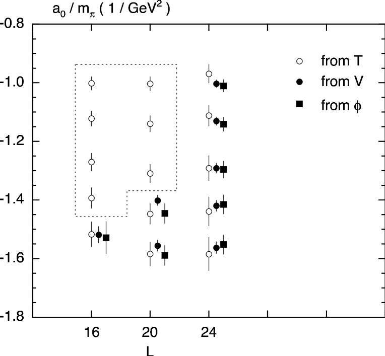
Figure 11: Volume dependence of pion scattering length $a_{0}/m_{\pi}\ (1/{\rm GeV}^{2})$ for five quark masses obtained from the time correlator (“from $T$”) and the wave function (“from $V$” and “from $\phi$”).

Our compilation of the the scattering lengths, i.e. those obtained on the three lattice volumes for five quark masses with three different methods, is depicted in Fig. 11. Data points encircled by dotted lines are those from the two-pion time correlator for the case for which we cannot clearly find a region $x<L/2$ where the two-pion interaction vanishes. We do not find a significant volume dependence, however, for all quark masses including the case where the necessary condition for Lüscher’s formula is not satisfied. The effects of deformation of the two-pion interaction due to finite volume effects on $\Delta W$ of the two-pion system are apparently small compared with the statistical error. We emphasize, however, that the reliability of these data is guaranteed only after we obtain the results on the $24^{3}$ lattice where the necessary condition for Lüscher’s formula is satisfied.

V Conclusions

We have shown in this work that calculations of the two-pion wave function for the ground state of the $I=2$ $S$-wave two-pion system is feasible. We have investigated the validity of the necessary condition for Lüscher’s formula and have found that it is satisfied for $L\geq 24$ ($3.92\ {\rm fm}$) for $m_{\pi}^{2}=0.273-0.736\ {\rm GeV}^{2}$. We have demonstrated that the scattering length can be extracted from the wave function with smaller statistical errors than from the two-pion time correlator which has been used in the studies to date.

We have observed no significant volume dependence for the scattering lengths obtained from the two-pion time correlator at least for $L\geq 16$ ($2.61\ {\rm fm}$), in spite of the fact that the necessary condition for the formula is not satisfied in some cases for $L=16$ and $20$. The effects of deformation of the two-pion interaction due to finite size effects on the energy eigenvalues of the two-pion are likely small compared with the statistical error.

The present work opens the possibility to reduce statistical errors in the scattering phase shift with modest statistics. In this case, however, we have to concern with the contamination from inelastic scattering. This effect is probably negligible for the ground state of the two-pion as in this work, but it may be important for the momentum excitation states, whose energies are close to the inelastic threshold. One may investigate effects of inelastic scattering by evaluating $I(\vec{x})$ in (37) in Appendix A from calculations of $\phi(\vec{x};k)$ and $\langle\pi(\vec{p})|\pi(-\vec{x}/2)|\pi\pi;k\rangle$. This would also clarify the error associated with our neglect of the inelastic channel, but the work is deferred to the future.

Another implication of the present work is the feasibility to calculate the decay width of the $\rho$ meson through studies of the $I=1$ two-pion system. While the evaluation of the disconnected diagrams with a good precision has been a computational problem, our new method, investigating the scattering system from the wave function of multi-hadron states in which the energy eigenvalue is extracted from the wave function at a single time slice, could lend a tactics that can be used to evaluate such complicated diagrams with a modest cost.

Appendix A Lüscher’s formula from Bethe-Salpeter wave function

We discuss the derivation of Lüscher’s formula (13) from Bethe-Salpeter (BS) wave function in quantum field theory LMST:kpp . All considerations are made in Minkowski space, but these are not changed even in Euclidian space.

We consider the BS function in the infinite volume defined by

$$\phi_{\infty}(\vec{x};\vec{k})=\langle 0|\pi_{1}(\vec{x}/2)\pi_{2}(-\vec{x}/2)|\pi_{1}(\vec{k}),\pi_{2}(-\vec{k});{\rm in}\rangle\ ,$$ (36)

where we consider the particle as distinguishable and denote two distinguishable pions by $\pi_{1}$ and $\pi_{2}$. The state $|\pi_{1}(\vec{k}),\pi_{2}(-\vec{k});{\rm in}\rangle$ is an asymptotic two-pion state with the momentum $\vec{k}$ and $-\vec{k}$, and $\pi_{1}(\vec{x})$ and $\pi_{2}(\vec{x})$ are the interpolating operators for the pion $\pi_{1}$ and $\pi_{2}$ at position $\vec{x}$. Inserting complete intermediate energy eigenstates between the two fields, we obtain

$$\phi_{\infty}(\vec{x};\vec{k})=\int\frac{{\rm d}^{3}p}{(2\pi)^{3}2E_{p}}\sqrt{Z}{\rm e}^{i\vec{p}\cdot\vec{x}/2}\langle\pi_{1}(\vec{p})|\pi_{2}(-\vec{x}/2)|\pi_{1}(\vec{k}),\pi_{2}(-\vec{k});{\rm in}\rangle+I(\vec{x})\ ,$$ (37)

where $E_{p}=\sqrt{m_{\pi}^{2}+p^{2}}$. $I(\vec{x})$ is contribution of in-elastic scattering from the states with more than one pions, whose contributions are expected to be small for the energy $2E_{k}<<4m_{\pi}$. This energy condition is satisfied for our case of the two-pion ground state, thus we neglect $I(\vec{x})$ in the following.

We decompose the BS function into the disconnected and the connected part, and rewrite them by the LSZ reduction formula as

$$\frac{\langle\pi_{1}(\vec{p})|\pi_{2}(-\vec{x}/2)|\pi_{1}(\vec{k}),\pi_{2}(-\vec{k});{\rm in}\rangle}{2E_{p}\sqrt{Z}{\rm e}^{i\vec{p}\cdot\vec{x}/2}}=(2\pi)^{3}\delta^{3}(\vec{p}-\vec{k})+\frac{H(p;k)}{p^{2}-k^{2}-i\epsilon}\ ,$$ (38)

where $H(p;k)$ is related to the off-shell two-pion scattering amplitude $M(p;k)$ by

$$H(p;k)=\frac{E_{p}+E_{k}}{8E_{p}E_{k}}M(p;k)\ .$$ (39)

$M(p;k)$ is defined from the pion 4-point Green function by

$${\rm e}^{-i{\bf q}\cdot{\bf x}}\frac{M(p;k)}{-{\bf q}^{2}+m_{\pi}^{2}-i\epsilon}=\int{\rm d}^{4}z\ {\rm d}^{4}y_{1}\ {\rm d}^{4}y_{2}\ {\bf K}({\bf p},{\bf z}){\bf K}(-{\bf k}_{1},{\bf y}_{1}){\bf K}(-{\bf k}_{2},{\bf y}_{2})$$ (40)

$$\qquad\qquad\qquad\qquad\qquad\qquad\qquad\qquad\langle 0|T\bigl{[}\pi_{1}({\bf z})\pi_{2}({\bf x})\pi_{1}({\bf y}_{1})\pi_{2}({\bf y}_{2})\bigr{]}|0\rangle\ ,$$ (41)

where all momenta and coordinates denoted by bold face characters refer to four-dimensional vectors and

$${\bf K}({\bf p},{\bf z})=\frac{i}{\sqrt{Z}}{\rm e}^{i{\bf p}\cdot{\bf z}}(-{\bf p}^{2}+m_{\pi}^{2})\ .$$ (42)

In our case the momenta in (41) take

$${\bf k}_{1}=(E_{k},\vec{k})\ ,\quad{\bf k}_{2}=(E_{k},-\vec{k})$$ (43)

$${\bf p}=(E_{p},\vec{p})\ ,\quad{\bf q}={\bf k}_{1}+{\bf k}_{2}-{\bf p}=(2E_{k}-E_{p},-\vec{p})\ .$$ (44)

${\bf q}$ is generally off-shell momentum and ${\bf q}=(E_{p},-\vec{p})$ at on-shell ($E_{p}=E_{k}$). The others are on-shell momenta.

We assume that the scattering phase shift $\delta_{l}(k)$ with $l\geq 1$ is negligible, and regard $H(p;k)$ and $M(p;k)$ as functions of $p=|\vec{p}|$ and $k=|\vec{k}|$. We also assume regularity for all $p$ and $k$. $M(p;k)$ and $H(p;k)$ are normalized as

$$M(k;k) = \frac{16\pi E_{k}}{k}{\rm e}^{i\delta_{0}(k)}\sin\delta_{0}(k)$$ (45)

$$H(k;k) = \frac{4\pi}{k}{\rm e}^{i\delta_{0}(k)}\sin\delta_{0}(k)$$ (46)

at on-shell $p=k$.

Substituting (38) into (37), we obtain

$$\phi_{\infty}(\vec{x};\vec{k}) = {\rm e}^{i\vec{k}\cdot\vec{x}}+\int\frac{{\rm d}^{3}p}{(2\pi)^{3}}\frac{H(p;k)}{p^{2}-k^{2}-i\epsilon}{\rm e}^{i\vec{p}\cdot\vec{x}}$$ (47)

$$= {\rm e}^{i\vec{k}\cdot\vec{x}}+\frac{ik}{4\pi}H(k;k)j_{0}(kx)+{\bf P}\int\frac{{\rm d}^{3}p}{(2\pi)^{3}}\frac{H(p;k)j_{0}(px)}{p^{2}-k^{2}}\ ,$$ (48)

where we neglect an irrelevant overall constant.

We assume

$$h(x;k) \equiv \int\frac{{\rm d}^{3}p}{(2\pi)^{3}}H(p;k){\rm e}^{-i\vec{p}\cdot\vec{x}}$$ (49)

$$= -(\triangle+k^{2})\phi_{\infty}(\vec{x};\vec{k})=0\qquad\mbox{ for $x>R$ }\ ,$$ (50)

where $h(x;k)$ depends only on $x=|\vec{x}|$ and $k=|\vec{k}|$. In order to simplify (48), we use a formula :

$${\bf P}\int\frac{{\rm d}^{3}p}{(2\pi)^{3}}\frac{F(p)}{p^{2}-k^{2}}=\int{\rm d}^{3}z\ f(z)\frac{k}{4\pi}n_{0}(kz)\ ,$$ (51)

where $f(z)$ is an inverse Fourier transformation of $F(p)$ which is a function of $p=|\vec{p}|$. From this the third term in (48) can be written by

$$E(x;k)\equiv{\bf P}\int\frac{{\rm d}^{3}p}{(2\pi)^{3}}\frac{H(p;k)j_{0}(px)}{p^{2}-k^{2}}=\int{\rm d}^{3}z\ g(z;k,x)\frac{k}{4\pi}n_{0}(kz)\ ,$$ (52)

where $g(z;k,x)$ is an inverse Fourier transformation of $H(p;k)j_{0}(px)$, which is given by

$$g(z;k,x) = \int\frac{{\rm d}^{3}p}{(2\pi)^{3}}H(p;k)j_{0}(px){\rm e}^{-i\vec{p}\cdot\vec{z}}$$ (53)

$$= \int\frac{{\rm d}\Omega_{x}}{4\pi}\int\frac{{\rm d}^{3}p}{(2\pi)^{3}}H(p;k){\rm e}^{i\vec{p}\cdot\vec{x}}{\rm e}^{-i\vec{p}\cdot\vec{z}}$$ (54)

$$= \int\frac{{\rm d}\Omega_{x}}{4\pi}\int{\rm d}^{3}y\,\delta^{3}(\vec{y}+\vec{x}-\vec{z})h(y;k)\ ,$$ (55)

with the spherical coordinate $\Omega_{x}$ for $\vec{x}$. By substituting (55) into (52), we obtain

$$E(x;k) = \int\frac{{\rm d}\Omega_{x}}{4\pi}\int{\rm d}^{3}y\ h(y;k)\frac{k}{4\pi}n_{0}(k|\vec{x}+\vec{y}|)$$ (56)

$$= \int_{0}^{\infty}{\rm d}y\ (4\pi y^{2})h(y;k)\int\frac{{\rm d}\Omega_{y}}{4\pi}\frac{k}{4\pi}n_{0}(k|\vec{x}+\vec{y}|)$$ (57)

$$= \int_{0}^{\infty}{\rm d}y\ (4\pi y^{2})h(y;k)\frac{k}{4\pi}\biggl{[}\Theta(x-y)\cdot n_{0}(kx)j_{0}(ky)$$ (59)

$$\qquad\qquad\qquad\qquad\qquad+\Theta(y-x)\cdot j_{0}(kx)n_{0}(ky)\biggr{]}\ ,$$

where $\Theta(x-y)$ is the step function, i.e. $\Theta(x-y)=1$ for $x-y\geq 0$ and $0$ for others. Under the assumption (50), (59) for $x>R$ can be written by

$$E(x;k) = \frac{k}{4\pi}n_{0}(kx)\int_{0}^{R}{\rm d}y\ (4\pi y^{2})h(y;k)j_{0}(ky)$$ (60)

$$= \frac{k}{4\pi}n_{0}(kx)\int_{0}^{\infty}{\rm d}y\ (4\pi y^{2})h(y;k)j_{0}(ky)$$ (61)

$$= \frac{k}{4\pi}n_{0}(kx)H(k;k)\ .$$ (62)

Now we achieve the following simple expression of the BS function in the infinite volume for $x>R$.

$$\phi_{\infty}(\vec{x};\vec{k}) = {\rm e}^{i\vec{k}\cdot\vec{x}}+\frac{ik}{4\pi}H(k;k)j_{0}(kx)+\frac{k}{4\pi}H(k;k)n_{0}(kx)$$ (63)

$$= \Bigl{[}{\rm e}^{i\vec{k}\cdot\vec{x}}-j_{0}(kx)\Bigr{]}+{\rm e}^{i\delta_{0}(k)}\cos\delta_{0}(k)j_{0}(kx)+{\rm e}^{i\delta_{0}(k)}\sin\delta_{0}(k)n_{0}(kx)\ ,$$ (64)

where we use the relation (46) in the final step.

The first term in (64) is written in terms of $j_{l}(kx)$ as

$${\rm e}^{i\vec{k}\cdot\vec{x}}-j_{0}(kx)=\sum_{l=1}^{\infty}\sum_{m=-l}^{l}(4\pi)i^{l}j_{l}(kx)Y_{lm}^{*}(\Omega_{k})Y_{lm}(\Omega_{x})\ ,$$ (65)

with the spherical coordinate $\Omega_{k}$ for $\vec{k}$ and $\Omega_{x}$ for $\vec{x}$. Thus it does not contain the $S$-wave component and it is a regular function for all $\vec{x}$. We find that the ratio of the coefficients of $j_{0}(kx)$ and $n_{0}(kx)$ in (64) gives the $S$-wave scattering phase shift. It should be noted that $\phi_{\infty}(\vec{x};\vec{k})$ does not contain $n_{l}(kx)$ with $l\geq 1$. This is attributed to the fact that we neglect the scattering phase shifts $\delta_{l}(k)$ with $l\geq 1$ and regard $M(p;k)$ as a function of $p=|\vec{p}|$ and $k=|\vec{k}|$.

The BS function on a periodic box $L^{3}$ is defined by

$$\phi(\vec{x};k)=\langle 0|\pi_{1}(\vec{x}/2)\pi_{2}(-\vec{x}/2)|\pi_{1}\pi_{2};k\rangle\ ,$$ (66)

where $|\pi_{1}\pi_{2};k\rangle$ is the energy eigenstate of two-pion system on the periodic box with energy $E=2\sqrt{m_{\pi}^{2}+k^{2}}$. Here we assume that the two-pion interaction range $R$ is smaller than one half of the lattice extent, i.e. $R<L/2$, so that the boundary condition does not distort the shape of $h(x;k)$.

$\phi(\vec{x};k)$ should be written in terms of $\phi_{\infty}(\vec{x};\vec{k})$ as follows.

$$\phi(\vec{x};k)=\sum_{l=0}^{\infty}\sum_{m=-l}^{l}C_{lm}\sqrt{4\pi}Y_{lm}(\Omega_{x})\phi^{lm}_{\infty}(x;k)\ ,$$ (67)

where $C_{lm}$ are determined from the boundary condition together with the allowed value of $k^{2}$, and $\phi^{lm}_{\infty}(x;k)$ is the $lm$ component of $\phi_{\infty}(\vec{x};\vec{k})$ defined by

$$\phi^{lm}_{\infty}(x;k)=\int\frac{{\rm d}\Omega_{x}}{4\pi}\sqrt{4\pi}Y_{lm}^{*}(\Omega_{x})\phi_{\infty}(\vec{x};\vec{k})\ .$$ (68)

$\phi(\vec{x};k)$ satisfies the the Helmholtz equation for $x>R$. The general solution of the equation on a periodic box $L^{3}$ can be written by (5) with $G_{lm}(\vec{x};k)$ defined by (7). Thus the equation (67) yields

$$\phi(\vec{x};k) = \sum_{l=0}^{\infty}\sum_{m=-l}^{l}C_{lm}\sqrt{4\pi}Y_{lm}(\Omega_{x})\phi^{lm}_{\infty}(x;k)$$ (69)

$$= \sum_{l=0}^{\infty}\sum_{m=-l}^{l}v_{lm}G_{lm}(\vec{x};k)\ ,$$ (70)

for $x>R$. As mentioned in Sec. II, $G_{lm}(\vec{x};k)$ contains $n_{l^{\prime}}(kx)$ with only $l^{\prime}=l$. $\phi_{\infty}(\vec{x};\vec{k})$ contains $n_{l}(kx)$ with only $l=0$ as known from (64) and (65). Thus only $v_{00}$ is non-zero and $G_{lm}(\vec{x};k)$ with $l\geq 1$ do not contribute in the second line of (70).

We use the expansion form of $G(\vec{x};k)$ given by (9) to determine the allowed value of $k^{2}$, $C_{lm}$ and $v_{00}$ in (70). Comparing the $S$-wave component of both lines of (70), we find

$$C_{00}\cdot{\rm e}^{i\delta_{0}(k)}\sin\delta_{0}(k)=v_{00}\cdot\frac{k}{4\pi}$$ (71)

$$C_{00}\cdot{\rm e}^{i\delta_{0}(k)}\cos\delta_{0}(k)=v_{00}\cdot g_{00}(k)\ .$$ (72)

Finally we obtain Lüscher’s formula (13) by taking the ratio of (71) and (72).

$$\frac{1}{\tan\delta_{0}(k)}=\frac{4\pi}{k}\cdot g_{00}(k)\ .$$ (73)

The other components of (70) give only the informations for $C_{lm}$.

Let us make a comment on the condition (50). In quantum field theory this condition is generally not exactly satisfied and there can be a small tail in $h(x;k)$ for large $x$. Thus we cannot rigorously define the two-pion interaction range. Further an exact estimation of the effects of the tail for the BS function is not possible, unless the off-shell two-pion scattering amplitude $H(p;k)$ for all $p$ for given $k$ is known. In this appendix we considered that the condition (50) is satisfied for some value of $R$, with a tacit assumption that the corrections from the interaction tails for the BS function are negligible.

Appendix B Numerical calculation of periodic Green function

We rewrite $G(\vec{x};k)$ in terms of dimensionless values as

$$(4\pi^{2}L)\cdot G(\vec{x};k)=\sum_{\vec{m}\in{\bf Z}^{3}}\frac{{\rm e}^{i\vec{m}\cdot\vec{X}}}{m^{2}-q_{k}^{2}}\ ,$$ (74)

where $q_{k}^{2}=k^{2}L^{2}/(2\pi)^{2}$ ($\not\in{\bf Z}$) and $\vec{X}=\vec{x}(2\pi)/L$. The function $G(\vec{x};k)$ can be expanded around the momentum $p^{2}=n_{p}^{2}\cdot(2\pi)^{2}/L^{2}$ ($n_{p}^{2}\in{\bf Z}$) as

$$(4\pi^{2}L)\cdot G(\vec{x};k)=-\frac{1}{q_{k}^{2}-n_{p}^{2}}\sum_{m^{2}=n_{p}^{2}}{\rm e}^{i\vec{m}\cdot\vec{X}}+\sum_{j=1}^{\infty}(q_{k}^{2}-n_{p}^{2})^{j-1}F(\vec{X};j,n_{p})\ ,$$ (75)

where

$$F(\vec{X};j,n_{p})=\sum_{m^{2}\not=n_{p}^{2}}(m^{2}-n_{p}^{2})^{-j}\ {\rm e}^{i\vec{m}\cdot\vec{X}}\ .$$ (76)

The function $F(\vec{X};j,n_{p})$ depends on the position $\vec{X}$, lattice geometry and the expansion point $n_{p}^{2}$. But it is independent of the physical quantity, such as quark masses and the strength of the two pion interaction. In our case of the ground state of the two-pion, we set $n_{p}^{2}=0$. We can use the same techniques as in Ref. CP-PACS:phsh_full for the evaluation of the spherical zeta function. $F(\vec{X};s,n_{p})$ takes finite values for ${\rm Re}(s)>3/2$. The function at $s=j\in{\bf Z}\geq 1$ is defined by the analytic continuation from this region.

First we divide the summation in $F(\vec{X};s,n_{p})$ into two parts as

$$F(\vec{X};s,n_{p})=\biggl{[}\ \sum_{m^{2}<n_{p}^{2}}+\sum_{m^{2}>n_{p}^{2}}\ \biggr{]}\ (m^{2}-n_{p}^{2})^{-s}\ {\rm e}^{i\vec{m}\cdot\vec{X}}\ .$$ (77)

The second part can be written by an integral form as

$$\sum_{m^{2}>n_{p}^{2}}\ (m^{2}-n_{p}^{2})^{-s}\ {\rm e}^{i\vec{m}\cdot\vec{X}}$$ (78)

$$=\biggl{(}\int_{0}^{\infty}{\rm d}t\sum_{m^{2}>n_{p}^{2}}\ \biggr{)}\frac{t^{s-1}}{\Gamma(s)}{\rm e}^{-t(m^{2}-n_{p}^{2})}{\rm e}^{i\vec{m}\cdot\vec{X}}$$ (79)

$$=\biggl{(}\int_{1}^{\infty}{\rm d}t\sum_{m^{2}>n_{p}^{2}}-\int_{0}^{1}{\rm d}t\sum_{m^{2}\leq n_{p}^{2}}+\int_{0}^{1}{\rm d}t\sum_{\vec{m}}\biggr{)}\frac{t^{s-1}}{\Gamma(s)}{\rm e}^{-t(m^{2}-n_{p}^{2})}{\rm e}^{i\vec{m}\cdot\vec{X}}\ .$$ (80)

The first and second terms in (80) converge at $s=j\in{\bf Z}\geq 1$, which are given by

$$-\frac{1}{j!}\sum_{m^{2}=n_{p}^{2}}{\rm e}^{i\vec{m}\cdot\vec{X}}-\sum_{m^{2}<n_{p}^{2}}\frac{{\rm e}^{i\vec{m}\cdot\vec{X}}}{(m^{2}-n_{p}^{2})^{j}}+\sum_{r=1}^{j}\frac{1}{(j-r)!}\sum_{m^{2}\not=n_{p}^{2}}\frac{{\rm e}^{-(m^{2}-n_{p}^{2})}}{(m^{2}-n_{p}^{2})^{r}}\ {\rm e}^{i\vec{m}\cdot\vec{X}}\ ,$$ (81)

at $s=j\in{\bf Z}\geq 1$. The third term in (80) is rewritten by Poisson’s summation formula :

$$\sum_{\vec{m}\in{\bf Z}^{3}}f(\vec{m})=\sum_{\vec{m}\in{\bf Z}^{3}}\int{\rm d}^{3}y\ f(\vec{y}){\rm e}^{i2\pi\vec{m}\cdot\vec{y}}\ ,$$ (82)

and integration over $\vec{y}$ yields,

$$\int_{0}^{1}{\rm d}t\sum_{\vec{m}\in{\bf Z}^{3}}\frac{t^{s-1}}{\Gamma(s)}{\rm e}^{-t(m^{2}-n_{p}^{2})}\ {\rm e}^{i\vec{m}\cdot\vec{X}}=\int_{0}^{1}{\rm d}t\frac{t^{s-1}}{\Gamma(s)}\biggl{(}\frac{\pi}{t}\biggr{)}^{3/2}\ {\rm e}^{tn_{p}^{2}}\sum_{\vec{m}\in{\bf Z}^{3}}{\rm e}^{-(\vec{X}+2\pi\vec{m})^{2}/(4t)}\ .$$ (83)

The final expression in (83) converges at $s=j\in{\bf Z}\geq 1$ for $\vec{X}/(2\pi)\not\in{\bf Z}^{3}$. We do not need the values at $\vec{X}/(2\pi)=\vec{n}\in{\bf Z}^{3}$, because these correspond to $\vec{x}=\vec{n}L$ and these positions are within the two-pion interaction range. Finally, gathering all terms and setting $s=j\in{\bf Z}\geq 1$ in (83), we obtain

$$F(\vec{X};j,n_{p})=-\frac{1}{j!}\sum_{m^{2}=n_{p}^{2}}{\rm e}^{i\vec{m}\cdot\vec{X}}+\sum_{r=1}^{j}\frac{1}{(j-r)!}\sum_{m^{2}\not=n_{p}^{2}}\frac{{\rm e}^{-(m^{2}-n_{p}^{2})}}{(m^{2}-n_{p}^{2})^{r}}\ {\rm e}^{i\vec{m}\cdot\vec{X}}$$ (84)

$$\qquad\qquad\qquad\qquad+\frac{\pi^{3/2}}{(j-1)!}\int_{0}^{1}{\rm d}t\ t^{j-5/2}\ {\rm e}^{tn_{p}^{2}}\sum_{\vec{m}}{\rm e}^{-(\vec{X}+2\pi\vec{m})^{2}/(4t)}\ \ \ .$$ (85)

Figure 1: Two-pion wave function $\phi(\vec{x};k)$ on $24^{3}$ lattice on $(t,z)=(52,0)$ plane for $m_{\pi}^{2}=0.273\ {\rm GeV}^{2}$. The reference vector is set at $\vec{x}_{0}=(7,5,2)$ ($x_{0}=|\vec{x}_{0}|=8.832$).

Figure 2: Two-pion wave function $\phi(\vec{x};k)$ on $24^{3}$ lattice at $t=52$ for $m_{\pi}^{2}=0.273\ {\rm GeV}^{2}$. Horizontal axis is $x=|\vec{x}|$. Filled symbols are data points and cross symbols are results of fitting with $G(\vec{x};k)$.

Figure 3: $V(\vec{x};k)$ in unit of $1/a^{2}$ on $24^{3}$ lattice on $(t,z)=(52,0)$ plane for $m_{\pi}^{2}=0.273\ {\rm GeV}^{2}$.

Figure 7: Effective mass for $R(t)$ on $24^{3}$ lattice in unit of $1/a$ at $m_{\pi}^{2}=0.273$ (lightest), $0.444$ and $0.736\ {\rm GeV}^{2}$ (heaviest).

Figure 10: $V(\vec{x};k)$ in unit of $1/a^{2}$ (left side) and $U(\vec{x};k)$ (right side) on $16^{3}$ lattice at $t=52$ for several quark masses. In left side of figures we also plot a line at $-k^{2}$ obtained from the two-pion time correlator. Horizontal axis is $x=|\vec{x}|$.

$L^{3}=24^{3}$
$m_{\pi}\ ({\rm GeV})$		$0.85773(27)$	$0.76675(28)$	$0.66649(30)$	$0.59205(31)$	$0.52290(33)$
$m_{\pi}^{2}\ ({\rm GeV}^{2})$		$0.73570(47)$	$0.58790(43)$	$0.44421(40)$	$0.35052(37)$	$0.27342(35)$
$x_{m}$		$9.8$	$9.8$	$9.8$	$9.4$	$9.0$
$\Delta W\ (\times 10^{-3}\ {\rm GeV})$
	from $T$	$1.748(64)$	$2.011(73)$	$2.337(86)$	$2.60(10)$	$2.85(11)$
	from $V$	$1.817(25)$	$2.049(29)$	$2.336(35)$	$2.559(37)$	$2.804(40)$
	from $\phi$	$1.832(43)$	$2.071(49)$	$2.346(58)$	$2.550(65)$	$2.784(66)$
$k^{2}\ (\times 10^{-3}\ {\rm GeV}^{2})$
	from $T$	$1.500(55)$	$1.543(56)$	$1.559(58)$	$1.540(59)$	$1.492(60)$
	from $V$	$1.559(22)$	$1.572(22)$	$1.558(23)$	$1.517(22)$	$1.468(21)$
	from $\phi$	$1.572(36)$	$1.589(38)$	$1.565(39)$	$1.512(39)$	$1.457(35)$
$a_{0}/m_{\pi}\ (1/{\rm GeV}^{2})$
	from $T$	$-0.969(32)$	$-1.112(36)$	$-1.291(42)$	$-1.439(49)$	$-1.585(57)$
	from $V$	$-1.003(12)$	$-1.131(14)$	$-1.291(17)$	$-1.420(18)$	$-1.562(20)$
	from $\phi$	$-1.010(21)$	$-1.141(24)$	$-1.296(29)$	$-1.415(32)$	$-1.552(33)$

Table 1: Results on $24^{3}$ lattice from two-pion time correlator (“from $T$”), constant fit of $V(\vec{x};k)$ (“from $V$”) and fitting wave function with $G(\vec{x};k)$ (“from $\phi$”). The fitting range of $V(\vec{x};k)$ and $\phi(\vec{x};k)$ are quoted as $x_{m}$.

$L^{3}=20^{3}$
$m_{\pi}\ ({\rm GeV})$		$0.85754(25)$	$0.76653(26)$	$0.66628(28)$	$0.59188(30)$	$0.52283(32)$
$m_{\pi}^{2}\ ({\rm GeV}^{2})$		$0.73537(42)$	$0.58757(40)$	$0.44393(38)$	$0.35033(36)$	$0.27335(34)$
$x_{m}$					$9.0$	$8.2$
$\Delta W\ (\times 10^{-3}\ {\rm GeV})$
	from $T$	$3.219(88)$	$3.66(10)$	$4.20(11)$	$4.63(13)$	$5.03(15)$
	from $V$				$4.457(63)$	$4.928(68)$
	from $\phi$				$4.62(12)$	$5.05(12)$
$k^{2}\ (\times 10^{-3}\ {\rm GeV}^{2})$
	from $T$	$2.763(76)$	$2.810(77)$	$2.805(76)$	$2.744(75)$	$2.635(78)$
	from $V$				$2.643(38)$	$2.583(36)$
	from $\phi$				$2.741(72)$	$2.646(64)$
$a_{0}/m_{\pi}\ (1/{\rm GeV}^{2})$
	from $T$	$-1.003(24)$	$-1.139(27)$	$-1.310(31)$	$-1.447(35)$	$-1.584(41)$
	from $V$				$-1.401(17)$	$-1.556(19)$
	from $\phi$				$-1.446(33)$	$-1.589(34)$

Table 2: Results on $20^{3}$ lattice from two-pion time correlator (“from $T$”), constant fit of $V(\vec{x};k)$ (“from $V$”) and fitting wave function with $G(\vec{x};k)$ (“from $\phi$”). The fitting range of $V(\vec{x};k)$ and $\phi(\vec{x};k)$ are quoted as $x_{m}$.

$L^{3}=16^{3}$
$m_{\pi}\ ({\rm GeV})$		$0.85759(34)$	$0.76672(37)$	$0.66660(41)$	$0.59225(45)$	$0.52318(50)$
$m_{\pi}^{2}\ ({\rm GeV}^{2})$		$0.73546(58)$	$0.58786(57)$	$0.44435(55)$	$0.35076(53)$	$0.27371(52)$
$x_{m}$						$7.8$
$\Delta W\ (\times 10^{-3}\ {\rm GeV})$
	from $T$	$6.51(17)$	$7.28(20)$	$8.20(23)$	$8.93(26)$	$9.62(32)$
	from $V$					$9.64(21)$
	from $\phi$					$9.71(41)$
$k^{2}\ (\times 10^{-3}\ {\rm GeV}^{2})$
	from $T$	$5.59(15)$	$5.59(15)$	$5.48(15)$	$5.31(16)$	$5.06(17)$
	from $V$					$5.07(11)$
	from $\phi$					$5.10(22)$
$a_{0}/m_{\pi}\ (1/{\rm GeV}^{2})$
	from $T$	$-1.002(22)$	$-1.122(26)$	$-1.270(30)$	$-1.393(35)$	$-1.517(43)$
	from $V$					$-1.519(28)$
	from $\phi$					$-1.528(55)$

Table 3: Results on $16^{3}$ lattice from two-pion time correlator (“from $T$”), constant fit of $V(\vec{x};k)$ (“from $V$”) and fitting wave function with $G(\vec{x};k)$ (“from $\phi$”). The fitting range of $V(\vec{x};k)$ and $\phi(\vec{x};k)$ are quoted as $x_{m}$.

References

(1)
S. Sharpe, R. Gupta and G.W. Kilcup,
Nucl. Phys. B383 (1992) 309.
(2)
R. Gupta, A. Patel and S. Sharpe,
Phys. Rev. D48 (1993) 388.
(3)
Y. Kuramashi, M. Fukugita, H. Mino, M. Okawa and A. Ukawa,
Phys. Rev. Lett. 71 (1993) 2387;
M. Fukugita, Y. Kuramashi, M. Okawa, H. Mino and A. Ukawa,
Phys. Rev. D52 (1995) 3003.
(8)
X. Du, G. Meng, C. Miao and C. Liu,
Int. J. Mod. Phys. A19 (2004) 5609.
(9)
BGR Collaboration, C. Gattringer, D. Hierl and R. Pullirsch,
Nucl. Phys. B(Proc. Suppl.)140 (2005) 308.
(10)
H.R. Fiebig, K. Rabitsch, H. Markum, and A. Mihály,
Nucl. Phys. B(Proc. Suppl.)73 (1999) 252;
Few-Body System, 29 (2000) 95.
(11)
CP-PACS Collaboration, S. Aoki et al.,
Phys. Rev. D67 (2003) 014502.
(12)
CP-PACS Collaboration, T. Yamazaki et al.,
Phys. Rev. D70 (2004) 074513.
(13)
C. Kim,
Nucl. Phys. B(Proc. Suppl.)129 (2004) 197;
Nucl. Phys. B(Proc. Suppl.)140 (2005) 381.
(14)
M. Lüscher, Commun. Math. Phys. 105 (1986) 153.
(15)
M. Lüscher,
Selected topics in lattice theory,
Lectures given at Les Houches (1988).
(16)
M. Lüscher and U. Wolff,
Nucl. Phys. B339 (1990) 222.
(17)
M. Lüscher,
Nucl. Phys. B354 (1991) 531.
(18)
J. Balog, M. Niedermaier, F. Niedermayer,
A. Patrascioiu, E. Seiler and P. Weisz,
Phys. Rev. D60 (1999) 094508;
Nucl. Phys. B618 (2001) 315.
(19)
C.-J.D. Lin, G. Martinelli, C.T. Sachrajda and M. Testa,
Nucl. Phys. B619 (2001) 467;
Nucl. Phys. B(Proc. Suppl.)109A (2002) 218.
(20)
T. Yamazaki,
Nucl. Phys. B(Proc. Suppl.)140 (2005) 338.
(21)
N. Ishizuka and T. Yamazaki,
Nucl. Phys. B(Proc. Suppl.)129 (2004) 233;
CP-PACS Collaboration, S. Aoki et al.,
Nucl. Phys. B(Proc. Suppl.)140 (2005) 305.
(22)
A. Messiah,
Quantum mechanics,
Vols. I, II ( North-Holland, Amsterdam, 1965 ).
(23)
Y. Iwasaki, Nucl. Phys. B258 (1985) 141;
University of Tsukuba Report No. UTHEP-118 (1983).
(24)
B. Sheikholeslami and R. Wohlert,
Nucl. Phys. B259 (1985) 572.
(25)
CP-PACS Collaboration, S. Aoki et al.,
Phys. Rev. D65 (2002) 054505.
(26)
C. Bernard and M. Golterman, J. Labrez, S. Sharpe and A. Ukawa,
Nucl. Phys. B(Proc. Suppl.)34 (1994) 334;
C. Bernard and M. Golterman,
Phys. Rev. D53 (1996) 476.
(27)
G. Colangelo and E. Pallante,
Nucl. Phys. B520 (1998) 433.
(28)
J. Gasser and H. Leutwyler,
Phys. Lett. B125 (1983) 325;
Annals. Phys. 158 (1984) 142;
J. Bijnens, G. Colangelo, G. Ecker, J. Gasser, and M.E. Sainio,
Phys. Lett. B374 (1996) 210;
Nucl. Phys. B508 (1997) 263;
G. Colangelo, J. Gasser, and H. Leutwyler
Nucl. Phys. B603 (2001) 125.