Search for the possible S=+1 Pentaquark states in Quenched Lattice QCD

Abstract

We study spin $\frac{1}{2}$ hadronic states in quenched lattice QCD to search for a possible $S=+1$ pentaquark resonance. Simulations are carried out on $8^{3}\times 24$, $10^{3}\times 24$, $12^{3}\times 24$ and $16^{3}\times 24$ lattices at $\beta$=5.7 at the quenched level with the standard plaquette gauge action and the Wilson quark action. We adopt a Dirichlet boundary condition in the time direction for the quark to circumvent the possible contaminations due to the (anti)periodic boundary condition for the quark field, which are peculiar to the pentaquark. By diagonalizing the $2\times 2$ correlation matrices constructed from two independent operators with the quantum numbers $(I,J)=(0,\frac{1}{2})$, we successfully obtain the energies of the lowest state and the 2nd-lowest state in this channel. The analysis of the volume dependence of the energies and spectral weight factors indicates that a resonance state is likely to exist slightly above the NK threshold in $(I,J^{P})=(0,\frac{1}{2}^{-})$ channel.

I Introduction

After the discovery Netal03 of $\Theta^{+}(1540)$ followed by the other experiments DIANA03 ; CLAS03 ; SAPHIR03 ; ZEUS04 ; ADK04 ; HERMES04 ; COSY04 ; CLAS04 , identifying the properties of the particle is one of the central problems in hadron physics. While the isospin of $\Theta^{+}$ is likely to be zero SAPHIR03 , the spin and the parity and the origin of its tiny width still remain open questions O04 ; J04 . In spite of many theoretical studies on $\Theta^{+}$ DPP97 ; P03 ; EMN04 ; H03 ; SDO04 ; O04 ; J04 , the nature of this exotic particle, including the very existence of the particle, is still controversial. Among theoretical approaches, the lattice QCD calculation is considered as one of the most reliable ab initio methods for studying the properties of hadronic states, which has been very successful in reproducing the non-exotic hadron mass spectra CPPACS01 . Up to now, several lattice QCD studies have been reported, which aim to look for pentaquarks in various different ways. However, the conclusions are unfortunately contradictory with each other. On one hand, the authors in Refs. CFKK03 ; S03 ; TTTT04 conclude that the parity of $\Theta^{+}$ is likely to be negative, while in Ref. CH04 the state with the similar mass to $\Theta^{+}$ in the positive parity channel is reported. In Refs. Metal04 ; IDIOOS04 , the absence of $\Theta^{+}$ is suggested.

One of the difficulties in the spectroscopy calculation with lattice QCD arises from the fact that the hadron masses suffer from systematic errors due to the discretization, the chiral extrapolation, the quenching effect, the finite volume effect and the contaminations from higher excited-states. The difficulty specific to the present problem is that the signal of $\Theta^{+}$ is embedded in the discrete spectrum of NK scattering states in finite volume. In order to verify the existence of a resonance state, one needs to isolate the first few low energy states including the lowest NK scattering state, identify a resonance state and study its volume dependence which can distinguish itself from other scattering states. Therefore, ideally one should extract multistates from a high statistics unquenched calculation for several different physical volumes, where both the continuum and the chiral limits are taken. However, due to enormous computational costs, so far there are no lattice QCD study which performs all these steps.

In the present situation where even the very existence of the resonance state is theoretically in dispute, the primary task is to provide evidences which distinguish the candidate resonance state from a scattering state. As long as other systematic errors only affect the numerical values of the masses but not the characteristic evidences of the resonance state, they may be neglected. Even so, the isolation of the first few low energy states and the study of the volume dependence is a minimum requisite.

Therefore, at this stage as a first step towards a more complete analysis, we propose to focus only on analyses using rather heavy quarks on coarse quenched lattices but with a good statistics. By such a strategy, we can afford taking several different lattice volumes with thousands of gauge configurations so that the careful separation of states and the studies of volume dependence are possible. Although giving well controlled continuum and chiral extrapolations may be important, we simply assume that the contents in spectra would not be drastically changed, although there are some cases where level crossings of resonance states occur as the quark masses decrease Metal05 . Even with such a compromise, we can hopefully learn about the existence and much of the qualitative properties of $\Theta^{+}$.

In this paper, we study $(I,J)=(0,\frac{1}{2})$ channel in quenched lattice QCD to search for possible resonance states. We adopt two independent operators with $I=0$ and $J=\frac{1}{2}$ and diagonalize the $2\times 2$ correlation matrices by the variational method for all the combinations of lattice sizes and quark masses to extract the 2nd-lowest state slightly above the NK threshold in this channel. After the careful separation of the states, we investigate the volume dependence of the energy as well as the spectral weight Metal04 of each state so that we can distinguish the resonance state from simple scattering states.

The paper is organized as follows. We present the formalism used in the analysis in Sec. II and show the simulation conditions in Sec. III. The process of the analysis is shown in Sec. IV. Secs. V-VIII are devoted to the interpretation of the obtained results and the verification of the existence of a resonance state, as well as some checks on the consistency and the reliability of the obtained data. In Sec. IX, we discuss the operator dependence of the results and compare our results with the previous works. We finally summarize the paper in Sec. X. In Appendix, we show the result of another trial to estimate the volume dependences of the spectral weights, which requires no multi-exponential fit.

II Formalism

As $\Theta^{+}$ lies above the NK threshold, any hadron correlators, which have the $\Theta^{+}$ signal, also contain the discrete-level NK scattering states in a finite volume lattice. In order to isolate the resonance state from the scattering states, one needs to extract at least two states before anything else.

Since a double-exponential fit of a single correlator becomes numerically ambiguous, we adopt the variational method using correlation matrices constructed from independent operators PM90 ; LW90 ; TS04 ; CH04 . A set of independent operators ,{$O_{\rm snk}^{I}$} for sinks and{$O_{\rm src}^{I\dagger}$} for sources, is needed to construct correlation matrices ${\cal C}^{IJ}(T)\equiv\langle O_{\rm snk}^{I}(T)O_{\rm src}^{J\dagger}(0)\rangle$, which can be decomposed into the sum over the energy eigenstates $|i\rangle$ as

$${\cal C}_{IJ}(T)=\langle O_{\rm snk}^{I}(T)O_{\rm src}^{J\dagger}(0)\rangle=\sum_{i}\sum_{j}C^{\dagger}_{{\rm snk}Ii}\Lambda(T)_{ij}C_{{\rm src}jJ},=(C^{\dagger}_{\rm snk}\Lambda(T)C_{\rm src})_{IJ},$$ (1)

with the general matrices which depend on the operators as

$$C^{\dagger}_{{\rm snk}Ii}\equiv\langle 0|O_{\rm snk}^{I}|i\rangle,C_{{\rm src}jI}\equiv\langle j|O_{\rm src}^{J\dagger}|0\rangle,$$ (2)

and the diagonal matrix

$$\Lambda(T)_{ij}\equiv\delta_{ij}e^{-E_{i}T}.$$ (3)

From the product

$${\cal C}^{-1}(T+1){\cal C}(T)=C_{\rm src}^{-1}\Lambda(-1)C_{\rm src},$$ (4)

we can extract the energies {$E_{i}$} as the logarithm of eigenvalues {$e^{E_{i}}$} of the matrix ${\cal C}^{-1}(T+1){\cal C}(T)$.

While there are $N$ independent operators for the correlation matrix, the number of the intermediate states $|i\rangle$ which effectively contribute to this matrix may differ from $N$ in general. Let us call this number as $N_{\rm eff}$. If $N_{\rm eff}$ is larger than $N$, the higher excited-states are non negligible and their contaminations give rise to a $T$-dependence of eigenvalues as {$e^{E_{i}(T)}$}. If on the other hand $N_{\rm eff}$ is smaller than $N$, ${\cal C}$ becomes non-invertible so that the extracted energies become numerically fairly unstable and we cannot extract all the $N$ eigenvalues. In order to have a reliable extraction of states, we therefore need to find an appropriate window of $T$ ($T_{\rm min}\leq T\leq T_{\rm max}$) so that $N_{\rm eff}=N$. (Of course, even in the case when $N>N_{\rm eff}$, we can extract $N_{\rm eff}$ eigenvalues with the reduced $N_{\rm eff}\times N_{\rm eff}$ correlation matrices.) The stability of {$e^{E_{i}(T)}$} against $T$ is expected in this $T$ range and we can obtain $N$ eigenenergies {$E_{i}$} ($0\leq i\leq N-1$) by fitting the eigenvalues $e^{E_{i}(T)}$ as $E_{i}=E_{i}(T)\equiv\ln(e^{E_{i}(T)})$ in $T_{\rm min}\leq T\leq T_{\rm max}$. Since finding the stability of the energies against $T$ in noisy data may suffer from uncontrollable biases, the result could be quite subjective. In order to avoid such biases, one should impose some concrete criteria to judge the stability as will be explained in later sections and select only those data which satisfy the criteria. After the separation of the states, we need to distinguish a possible resonance state from NK scattering states by the volume dependence of each state. It is expected that the energies of resonance states have small volume dependence, while the energies of NK scattering states are expected to scale as $\sqrt{M_{N}^{2}+|\frac{2\pi}{L}\vec{\bf n}|^{2}}+\sqrt{M_{K}^{2}+|\frac{2\pi}{L}\vec{\bf n}|^{2}}$ according to the relative momentum $\frac{2\pi}{L}\vec{\bf n}$ between N and K on a finite periodic lattice, provided that the NK interaction is weak and negligible which is indeed the case for the leading order in chiral perturbation theory.

Although the variational method is powerful for extracting the energy spectrum, one can obtain only part of the information on the spectral weights $C$. In order to extract the spectral weights, we also perform constrained double exponential fits using the energies from the variational method as inputs.

III Lattice set up

We carry out simulations on four different sizes of lattices, $8^{3}\times 24$, $10^{3}\times 24$, $12^{3}\times 24$ and $16^{3}\times 24$ with 2900, 2900, 1950 and 950 gauge configurations using the standard plaquette (Wilson) gauge action at $\beta=5.7$ and the Wilson quark action. The hopping parameters for the quarks are $(\kappa_{u,d},\kappa_{s})$=$(0.1600,0.1650)$, $(0.1625,0.1650)$, $(0.1650,0.1650)$, $(0.1600,0.1600)$ and $(0.1650,0.1600)$, which correspond to the current quark masses $(m_{u,d},m_{s})\sim(240,100)$, $(170,100)$, $(100,100)$, $(240,240)$ and $(100,240)$, respectively in the unit of MeV BCSVW94 . The lattice spacing $a$ from the Sommer scale is set to be 0.17 fm, which implies the physical lattice sizes are $1.4^{3}\times 4.0$ fm⁴, $1.7^{3}\times 4.0$ fm⁴, $2.0^{3}\times 4.0$ fm⁴ and $2.7^{3}\times 4.0$ fm⁴.

We adopt the following two operators used in Ref. CFKK03 for the interpolating operators at the sink $\{O_{\rm snk}^{I}\}$;

$$\Theta^{1}(x)\equiv\varepsilon^{abc}[u_{a}^{\rm T}(x)C\gamma_{5}d_{b}(x)]\{u_{e}(x)[{\overline{s_{e}}(x)\gamma_{5}d_{c}(x)}]-(u\leftrightarrow d)\},$$ (5)

which is expected to have a larger overlap with $\Theta^{+}$ state, and

$$\Theta^{2}(x)\equiv\varepsilon^{abc}[u_{a}^{\rm T}(x)C\gamma_{5}d_{b}(x)]\{u_{c}(x)[{\overline{s_{e}}(x)\gamma_{5}d_{e}(x)}]-(u\leftrightarrow d)\},$$ (6)

which we expect to have larger overlaps with NK scattering states. Here, the Dirac fields $u(x)$, $d(x)$ and $s(x)$ are up, down and strange quark fields, respectively and the Roman alphabets {a,b,c,e} denote color indices. For measuring the energy spectrum, the two operators at the source $\{O_{\rm src}^{I\dagger}\}$ are chosen to be $\Theta^{1}_{\rm wall}(t)$ and $\Theta^{2}_{\rm wall}(t)$ defined using spatially spread quark fields $\sum_{\vec{\bf x}}q(x)$ with the Coulomb gauge:

$$\Theta^{1}_{\rm wall}(t) \equiv \left(\sqrt{\frac{1}{V}}\right)^{5}\sum_{\vec{\bf x_{1}}\sim\vec{\bf x_{5}}}\varepsilon^{abc}[u_{a}^{\rm T}(x_{1})C\gamma_{5}d_{b}(x_{2})]\{u_{e}(x_{3})[{\overline{s_{e}}(x_{4})\gamma_{5}d_{c}(x_{5})}]-(u\leftrightarrow d)\},$$ (7)

and

$$\Theta^{2}_{\rm wall}(t)\equiv\left(\sqrt{\frac{1}{V}}\right)^{5}\sum_{\vec{\bf x_{1}}\sim\vec{\bf x_{5}}}\varepsilon^{abc}[u_{a}^{\rm T}(x_{1})C\gamma_{5}d_{b}(x_{2})]\{u_{c}(x_{3})[{\overline{s_{e}}(x_{4})\gamma_{5}d_{e}(x_{5})}]-(u\leftrightarrow d)\}.$$ (8)

The above operators give a $2\times 2$ correlation matrix in the channel with the quantum number of $(I,J)=(0,\frac{1}{2})$. We note here that the baryonic correlators have the spinor indices, which we omit in the paper, and they contain the propagations of both the positive and negative parity particles. For the parity projection, we simply multiply the correlators by $\frac{1}{2}(1\pm\gamma_{0})$ and extract the contributions proportional to $(1\pm\gamma_{0})$ from the negative-parity and positive-parity particles, respectively.

We fix the source operator $\overline{\Theta}_{\rm wall}(t)$ on $t=t_{\rm src}\equiv 6$ plane to reduce the effect of the Dirichlet boundary on $t=0$ plane CPPACS04 ; CPPACS95 . We adopt the operators $\sum_{\vec{\bf x}}\Theta^{I}(\vec{\bf x},t)$ as sink operators, which is summed over all space to project out the zero-momentum states. We finally calculate

$${\cal C}^{IJ}(T)=\sum_{\vec{\bf x}}\langle\Theta^{I}(\vec{\bf x},T+t_{\rm src})\overline{\Theta^{J}}_{\rm wall}(t_{\rm src})\rangle.$$ (9)

Using two independent operators, we can extract the first two states, namely the lowest and the next-lowest states. The lowest state is considered to be the “lowest” NK scattering state. In order to extract a possible resonance state with controlled systematic errors, we need to choose the physical volume of the lattice in an appropriate range. If we choose $L$ to be too large, the resonance state becomes heavier than the 2nd-lowest NK scattering state whose energy is naively expected to scale as $\sqrt{M_{N}^{2}+(\frac{2\pi}{L})^{2}}+\sqrt{M_{K}^{2}+(\frac{2\pi}{L})^{2}}$ according to the spatial lattice extent $L$. In this case we need to extract the 3rd state using a $3\times 3$ correlation matrix, which requires more computational time. The energy difference between the lowest and the next-lowest NK scattering states $\sqrt{M_{N}^{2}+(\frac{2\pi}{L})^{2}}+\sqrt{M_{K}^{2}+(\frac{2\pi}{L})^{2}}-(M_{N}+M_{K})$, for example, ranges from 180 MeV to 860 MeV in $1.4{\rm fm}\leq L\leq 3.5{\rm fm}$. Taking into account that $\Theta^{+}$ lies about 100 MeV above the NK threshold, we take 3.5 fm as the upper limit of $L$. On the other hand, if we choose $L$ too small, unwanted finite-volume artifacts from the finite sizes of particles become non-negligible. It is however difficult to estimate the lower limit of $L$, because the finite-volume effect is rather uncontrollable. We shall take the spatial extents $L=8,10,12,16$ at $\beta=5.7$ as a trial.

We take periodic boundary conditions in all directions for the gauge field, whereas we impose periodic boundary conditions on the spatial directions and the Dirichlet boundary condition on the temporal direction for the quark field in order to avoid possible contaminations from those propagating beyond the boundary at $t=0$ in (anti)periodic boundary conditions. Since the source of possible contaminations is peculiar to the pentaquark and has not been properly noticed in previous studies, it is worthwhile to dwell on this problem for a moment.

Let us denote the correlators in the pentaquark channel with periodic/antiperiodic boundary conditions and Dirichlet boundary conditions as ${\cal C}_{P/AP}(T)$ and ${\cal C}_{D}(T)$, respectively. Inserting complete set of states these correlators read

$${\cal C}_{P/AP}(T) = \sum_{m,n}(-)^{\epsilon_{n}}\langle n|\Theta|m\rangle\langle m|\overline{\Theta}|n\rangle e^{-E_{m}T-E_{n}(N_{t}-T)},$$

$${\cal C}_{D}(T) = \sum_{m,n_{f},n_{i}}\langle D|n_{f}\rangle\langle n_{f}|\Theta|m\rangle\langle m|\overline{\Theta}|n_{i}\rangle\langle n_{i}|D\rangle e^{-E_{m}T-E_{n_{f}}(N_{t}-(T+t_{\rm src}))-E_{n_{i}}t_{\rm src}},$$ (10)

where the states $|m\rangle,\ |n\rangle,\ |n_{i}\rangle,\ |n_{f}\rangle$ are the eigenstates with energies $E_{m}$, $E_{n}$, $E_{n_{i}}$, $E_{n_{f}}$ respectively. $|D\rangle$ is the state which corresponds to the Dirichlet boundary condition and $(-)^{\epsilon_{n}}$ is the factor which represents the $\pm$ sign with antiperiodic boundary condition. The factor $(-)^{\epsilon_{n}}$ is equal to $1(-1)$ when $|n\rangle$ contains an even(odd) number of valence quarks. It should be noted that the up, down, and strange quark numbers $U,D,S$ for the state $|D\rangle$ are restricted to zero since all the quark fields $\psi({\bf x},0)$ are set to zero in Dirichlet boundary condition, while there is no restriction in the quark sector for the states $|n\rangle$ which appear in periodic/antiperiodic boundary conditions. This means that the following states can contribute in the correlators

$$|n\rangle= \mbox{any states including }|0\rangle,|\bar{K}\rangle,|\bar{N}\rangle,|\bar{N}\bar{K}\rangle\cdots \mbox{for periodic/antiperiodic b.c.},$$

$$|n_{i,f}\rangle= \mbox{any states(with $U=D=S=0$) including }|0\rangle\cdots \mbox{for Dirichlet b.c.},$$ (11)

where $|\bar{K}\rangle$ and $|\bar{N}\rangle$ are the antiparticle states of $|K\rangle$ and $|N\rangle$, respectively. Therefore, the correlators have the contributions in the long range limit,

$${\cal C}_{P/AP}(T) \sim \langle 0|\Theta|NK\rangle\langle NK|\overline{\Theta}|0\rangle e^{-E_{NK}T}+\langle 0|\Theta|\Theta\rangle\langle\Theta|\overline{\Theta}|0\rangle e^{-E_{\Theta}T}+\langle\bar{K}|\Theta|N\rangle\langle N|\overline{\Theta}|\bar{K}\rangle e^{-E_{N}T-E_{\bar{K}}(N_{t}-T)}$$ (12)

$$\pm\langle\bar{N}|\Theta|K\rangle\langle K|\overline{\Theta}|\bar{N}\rangle e^{-E_{K}T-E_{\bar{N}}(N_{t}-T)}\pm\langle\bar{N}\bar{K}|\Theta|0\rangle\langle 0|\overline{\Theta}|\bar{N}\bar{K}\rangle e^{-E_{\bar{N}\bar{K}}(N_{t}-T)}$$

$$+\mbox{ and excited states },$$

$${\cal C}_{D}(T) \sim \langle D|0\rangle\langle 0|\Theta|NK\rangle\langle NK|\overline{\Theta}|0\rangle\langle 0|D\rangle e^{-E_{NK}T}+\langle D|0\rangle\langle 0|\Theta|\Theta\rangle\langle\Theta|\overline{\Theta}|0\rangle\langle 0|D\rangle e^{-E_{\Theta}T}$$ (13)

$$+\mbox{ and excited states }.$$

In Fig. 1, we give a schematic picture of the contributions to the correlators. The first two terms in Eq.(12) are the contributions from the five quark states as given in diagram (A). The third, the fourth and the fifth terms in Eq.(12) which correspond to diagrams (C),(D) and (B) are hadronic contributions which propagate beyond the boundary.

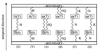
Figure 1: Schematic figure for the explanation on the possible contaminations of the particles propagating over the temporal boundary. $H(t)$ and $\Theta(t)$ are the interpolating operators and their arguments are the distances from the source point. $H(t)$ is a generic hadronic operator, which creates and annihilates the particles which cannot decay in quenched QCD. The wave lines represent the propagations of states. Resonance states like $\Theta^{+}$ are represented by “5Q” in the figure, as well as NK scattering states. The five-quark state can dissociate into forward-propagating nucleon (Kaon) and backward-propagating Kaon (nucleon).

As a result, the correlation $\langle\Theta(T+t_{\rm src})\overline{\Theta}(t_{\rm src})\rangle$ inevitably contains unwanted contributions such as

$$\langle\bar{K}|\Theta(T+t_{\rm src})|N\rangle\langle N|\overline{\Theta}(t_{\rm src})|\bar{K}\rangle\sim e^{-E_{N}T+E_{\bar{K}}(T-N_{t})}.$$ (14)

In this case, the effective mass plot approaches $E_{N}-E_{\bar{K}}$ below the NK threshold as $T$ is increased. On the other hand, the contributions corresponding to diagrams (C),(D) and (B) do not exist with Dirichlet boundary conditions (Eq.(13)). Therefore, we find that it would be safest to impose the Dirichlet boundary condition on the temporal direction, since no quark can go over the boundary on t=0 in the temporal direction. Although the boundary is transparent for the particles composed only by gluons; i.e. glueballs, due to the periodicity of the gauge action, it would be however safe to neglect these gluonic particles going beyond the boundary since these particles are rather heavy. Then, the correlation $\langle\Theta(T+t_{\rm src})\overline{\Theta}(t_{\rm src})\rangle$ mainly contains only such terms ((A) in Fig. 1) as

$$\langle{\rm vac}|\Theta(T+t_{\rm src})|{\rm 5Q}\rangle\langle{\rm 5Q}|\overline{\Theta}(t_{\rm src})|{\rm vac}\rangle=(1-\gamma_{0})\sum_{i}W^{+}_{i}e^{-E^{+}_{i}T}+(1+\gamma_{0})\sum_{i}W^{-}_{i}e^{-E^{-}_{i}T}$$ (15)

with $W^{\pm}_{i}$ the weight factor and $E^{\pm}_{i}$ the eigenenergy of $i$-th state in positive/negative parity channel, respectively. One sees that one can now apply the prescription mentioned in the last section.

One may wonder if these contaminations can be discarded with the parity projection of the correlators by taking linear combinations with periodic and antiperiodic boundary conditions. This method indeed works for ordinary three quark states where one can single out one of the two contributions diagram (X) and (Y) in Fig. 1. However even if one takes such linear combinations, one cannot make the contributions from diagram (C) seen in Eq.(12) cancel out as opposed to the contributions from diagram (B) and (D). It is because of the fact that the factor $(-)^{\epsilon_{n}}$ for the contribution (C) is always equal to $1$. (We note here that we can avoid these contaminations using the “averaged quark propagator” SS05 .) Some of the previous lattice QCD studies on $\Theta^{+}$ adopted a parity projection method using the combination with periodic and antiperiodic boundary conditions CFKK03 ; Metal04 . We stress that one should in principle be careful whether the result is free from the contamination owing to the boundary condition which is peculiar to the pentaquark and can mimic a fake plateau in the propagator.

After obtaining the energy spectrum, we carry out a study of the spectral weight for $(\kappa_{u,d},\kappa_{s})$=$(0.1600,0.1600)$. Introducing two smeared operators $\overline{\Theta^{1}}_{\rm smear}$, $\overline{\Theta^{2}}_{\rm smear}$ we compute the following correlators

$${\cal C}^{IJ}(T)=\sum_{\vec{\bf x}}\langle\Theta^{I}(\vec{\bf x},T+t_{\rm src})\overline{\Theta^{J}}_{\rm smear}(t_{\rm src})\rangle,$$ (16)

from which we extract the spectral weights using a constrained double exponential fit. The details will be explained in Sec. VII.

IV Lattice QCD data

Figure 2: The “effective mass” plot $E_{i}(T)$ as the function of $T$, the separation between source operators and sink operators, in $(I,J^{P})=(0,1/2^{-})$ channel with the hopping parameters $(\kappa_{u,d},\kappa_{s})=(0.1600.0.1600)$ on $8^{3}\times 24$, $10^{3}\times 24$, $12^{3}\times 24$,$16^{3}\times 24$ lattice at $\beta=5.7$. The stability of each $E_{i}(T)$ against $T$ means the smallness of the unwanted higher excited-state contaminations. The solid line and the dashed lines represent the central value and the error of the fitted masses $E_{0}^{-}$ and $E_{1}^{-}$.

Figure 3: The “effective mass” plot $E_{i}(T)$ as the function of $T$, the separation between source operators and sink operators, in $(I,J^{P})=(0,1/2^{-})$ channel with the hopping parameters $(\kappa_{u,d},\kappa_{s})=(0.1600.0.1650)$ on $8^{3}\times 24$, $10^{3}\times 24$, $12^{3}\times 24$,$16^{3}\times 24$ lattice at $\beta=5.7$.

Figure 4: The “effective mass” plot $E_{i}(T)$ as the function of $T$, the separation between source operators and sink operators, in $(I,J^{P})=(0,1/2^{-})$ channel with the hopping parameters $(\kappa_{u,d},\kappa_{s})=(0.1650.0.1600)$ on $8^{3}\times 24$, $10^{3}\times 24$, $12^{3}\times 24$,$16^{3}\times 24$ lattice at $\beta=5.7$.

Figure 5: The “effective mass” plot $E_{i}(T)$ as the function of $T$, the separation between source operators and sink operators, in $(I,J^{P})=(0,1/2^{-})$ channel with the hopping parameters $(\kappa_{u,d},\kappa_{s})=(0.1625.0.1650)$ on $8^{3}\times 24$, $10^{3}\times 24$, $12^{3}\times 24$,$16^{3}\times 24$ lattice at $\beta=5.7$.

Figure 6: The “effective mass” plot $E_{i}(T)$ as the function of $T$, the separation between source operators and sink operators, in $(I,J^{P})=(0,1/2^{-})$ channel with the hopping parameters $(\kappa_{u,d},\kappa_{s})=(0.1650.0.1650)$ on $8^{3}\times 24$, $10^{3}\times 24$, $12^{3}\times 24$,$16^{3}\times 24$ lattice at $\beta=5.7$.

Before obtaining the energies of the lowest state and the 2nd-lowest state, there are only a few simple steps. First, we calculate the $2\times 2$ correlation matrix ${\cal C}(T)$ defined in Eq.(9) and obtain the “energies” {$E_{i}(T)$} as the logarithm of eigenvalues {$e^{E_{i}(T)}$} of the matrix product ${\cal C}^{-1}(T+1){\cal C}(T)$. After finding the $T$ range ($T_{\rm min}\leq T\leq T_{\rm max}$), where {$E_{i}(T)$} are stable against $T$, we can extract the energies $E_{i}$ by the least $\chi$-squared fit of the data as $E_{i}=E_{i}(T)$ in $T_{\rm min}\leq T\leq T_{\rm max}$.

Since the volume dependence of the energy is crucial to judge whether the state is a resonance or not, a great care must be paid in extracting the energy. Therefore, the systematic error by the contaminations from higher excited-states should be avoided by a careful choice of fitting ranges. For this reason, we impose the following criteria for the reliable extraction of the energies. Although this set of the criteria is nothing more than just one possible choice, we believe it is important to impose some concrete criteria for the fit so that we can reduce the human bias for the fit, though not completely.

1. The effective mass plot should have “plateau” for both the lowest and the 2nd-lowest states simultaneously in a fit range [$T_{\rm min}$, $T_{\rm max}$], where the length $N_{\rm fit}\equiv T_{\rm max}-T_{\rm min}+1$ should be larger than or equal to 3 ( $N_{\rm fit}\geq 3$ ).

2. In the plateau region, the signal for the lowest and the 2nd-lowest states should be distinguishable, so that the gap between the central values of the lowest and the 2nd-lowest energies should be larger than their errors.

3. The fitted energies should be stable against the choice of the fit range; i.e. the results of the fit with $N_{\rm fit}$ time slices and with $N_{\rm fit}-1$ time slices should be consistent within statistical errors for both the lowest and the 2nd-lowest states.

4. The lowest state energy obtained by the diagonalization method using the $2\times 2$ correlation matrix should be consistent with the value from a single exponential fit for a sufficiently large $t$.

If the fit does not satisfy the above conditions, we discard the result since either the data in the fit range may be contaminated by higher excited-states or the 2nd-lowest-state signal is too noisy for a reliable fit.

Figs 2 show the “effective mass” plot $E_{i}(T)$ for the heaviest combination of quarks $(\kappa_{u,d},\kappa_{s})=(0.1600.0.1600)$. As is mentioned in Sec. II, we need to find the $T$ region ($T_{\rm min}\leq T\leq T_{\rm max}$) where each $E_{i}(T)$ shows a plateau. In the case of $12^{3}\times 24$ lattice in Fig. 2, for example, we choose the fit range of $T_{\rm min}=6$ and $T_{\rm max}=9$ ($N_{\rm fit}=4$). Notice that the source operators are put on the time slice with $t=t_{\rm src}=6$. The plateau in this region satisfies the above criteria so that we consider the fit $E_{0}^{-}$ and $E_{1}^{-}$ for the range $6\leq T\leq 9$ as being reliable. The situation is similar for the cases of $10^{3}\times 24$ and $16^{3}\times 24$ lattices. On the other hand, in the case of $8^{3}\times 24$ lattice we do not find a plateau region satisfying the above criteria.

Figs. 4,4,6,6 shows the “effective mass” plots for the combinations with smaller quark masses. We find that the signal is noisier for the lighter quarks and the fit with the smaller volumes $8^{3}\times 24$ and $10^{3}\times 24$ lattices do not satisfy the criteria.

V Lowest-state energy in $(I,J^{P})=(0,\frac{1}{2}^{-})$ channel

V.1 The volume dependence of the lowest-state energy

Now we show the lattice QCD results of the lowest state in $I=0$ and $J^{P}=\frac{1}{2}^{-}$ channel. The filled circles in Fig. 7 show the lowest-state energies $E_{0}^{-}$ in $I=0$ and $J^{P}=\frac{1}{2}^{-}$ channel on four different volumes. Here the horizontal axis denotes the lattice extent $L$ in the lattice unit and the vertical axis is the energy of the state. The lower line denotes the simple sum $M_{N}+M_{K}$ of the nucleon mass $M_{N}$ and Kaon mass $M_{K}$ obtained with the largest lattice. Though $M_{N}$ and $M_{K}$ are slightly affected by finite volume effects, the deviation of $M_{N}+M_{K}\ (L=8)$ from $M_{N}+M_{K}\ (L=16)$ is about a few % (Table 1.). We therefore simply use $M_{N}+M_{K}\ (L=16)$ as a guideline.

At a glance, we find that the energy of this state takes almost constant value against the volume variation and coincides with the simple sum $M_{N}+M_{K}$. We can therefore conclude that the lowest state in $I=0$ and $J^{P}=\frac{1}{2}^{-}$ channel is the NK scattering state with the relative momentum $|{\bf p}|=0$. The good agreement with the sum $M_{N}+M_{K}$ implies the weakness of the interaction between N and K. In fact, the scattering length in the $I=0$ channel is known to be tiny ( $a_{0}^{KN}(I=0)=-0.0075$ fm ) from compilations of hadron scattering experiments Dumbrajs:1983jd ; Nagels:1979xh , whereas the current algebra prediction from PCAC with SU(3) symmetry predicts that the scattering length $a_{0}^{KN}(I=0)=0$.

V.2 Comparison with the previous lattice work

We here compare our data with the previous lattice QCD studies, which were performed with almost the same conditions as ours, in order to confirm the reliability of our data.

The well-known hadron masses $m_{\pi}$,$m_{K}$ and $m_{N}$ listed in Table 1 can be compared with the values in Ref. BCSVW94 . Our data are consistent with those in Ref. BCSVW94 . The lowest NK scattering state in $(I,J^{P})=(0,\frac{1}{2}^{-})$ channel is carefully investigated in Ref. CPPACS95 with almost the same parameters as our present study. It is worth comparing our data with them. For the complete check of our data, we re-extract the lowest state by the ordinary single-exponential fit of the correlator as $\langle\Theta(T+t_{\rm src})\overline{\Theta}_{\rm wall}(t_{\rm src})\rangle=Ce^{-E_{NK}T}$ in the large-T region, and compare them with the present lattice data $E_{0}^{-}$ obtained by the multi-exponential method as well as the data in Ref. CPPACS95 . In Table 1, we list the data of the lowest state $E_{NK}$ obtained by the single-exponential fit. They almost coincide with the present data $E_{0}^{-}$ extracted by the multi-exponential method with about 1% deviations, which may be considered as the slightly remaining contaminations of the higher excited-state. In Ref. CPPACS95 , the authors extracted the energy difference $\delta E=E_{NK}-(E_{N}+E_{K})$ with the hopping parameters $\kappa_{u,d,s}=0.1640$ using $12^{3}\times 20$ lattice. We therefore compare our data $\delta E=E_{NK}-(E_{N}+E_{K})$ obtained with the hopping parameters $(\kappa_{u,d},\kappa_{s})=(0.1650,0.1650)$ on $12^{3}\times 24$ lattice. The energy difference $\delta E$ in our study is found to be $\delta E=-0.0128(38)$, which is consistent with the value of $-0.0051(38)$ in Ref. CPPACS95 taking into account that this error includes only statistical one.

It is now confirmed that the lowest state extracted using the multi-exponential method is consistent with the previous works and that our data and method are reliable enough to investigate the 2nd-lowest state in this channel.

VI 2nd-lowest state energy in $(I,J^{P})=(0,\frac{1}{2}^{-})$ channel

The $(I,J^{P})=(0,\frac{1}{2}^{-})$ state is one of the candidates for $\Theta^{+}(1540)$. Since $\Theta^{+}$ is located above the NK threshold, it would appear as an excited state in this channel. We show the lattice data of the 2nd-lowest state in this channel.

In order to distinguish a possible resonance state from NK scattering states, we investigate the volume dependence of both the energy and the spectral weight of each state. It is expected that the energies of resonance states have small volume dependence, while the energies of NK scattering states are expected to scale as $\sqrt{M_{N}^{2}+|\frac{2\pi}{L}\vec{\bf n}|^{2}}+\sqrt{M_{K}^{2}+|\frac{2\pi}{L}\vec{\bf n}|^{2}}$ according to the relative momentum $\frac{2\pi}{L}\vec{\bf n}$ between N and K on a finite periodic lattice, provided that the NK interaction is weak and negligible. We can take advantage of the above difference for the discrimination.

VI.1 Possible corrections to the volume dependence of NK scattering states

A possible candidate for the volume dependence of the energies of NK scattering states is the simple formula as $E_{NK}^{\vec{\bf n}}(L)\equiv\sqrt{M_{N}^{2}+|\frac{2\pi}{L}\vec{\bf n}|^{2}}+\sqrt{M_{K}^{2}+|\frac{2\pi}{L}\vec{\bf n}|^{2}}$ with the relative momentum $\frac{2\pi}{L}\vec{\bf n}$ between N and K in finite periodic lattices, which is justified on the assumption that nucleon and Kaon are point particles and that the interaction between them is negligible. In practice, there may be some corrections to the volume dependence of $E_{NK}^{\vec{\bf n}}(L)$. We therefore estimate here three possible corrections; the existence of the NK interaction, the application of the momenta on a finite discretized lattice and the estimation of the implicit finite-size effects.

There can be small hadronic interactions between nucleon and Kaon, which may lead to correction to naively expected energy spectrum $E_{NK}^{\vec{\bf n}}(L)$ of the NK scattering states. Using Lüscher formula L91 , one can relate the scattering phase shift to the energy shift from $E_{NK}^{\vec{\bf n}}(L)$ on finite lattices. For example, in the case when a system belongs to the representation ${\cal A}_{1}^{+}$ of cubic groups, which is relevant in the present case, the relation between the phase shift and the possible momentum spectra is

$$e^{2i\delta_{0}(k)}=\frac{{\cal Z}(1;q^{2})+i\pi^{\frac{2}{3}}q}{{\cal Z}(1;q^{2})-i\pi^{\frac{2}{3}}q}.$$ (17)

Here ${\cal Z}(s;q^{2})$ is the Zeta function defined as

$${\cal Z}(s;q^{2})\equiv\frac{1}{\sqrt{4\pi}}\sum_{n\in Z^{3}}\frac{1}{(n^{2}-q^{2})^{s}},$$ (18)

with the eigenenergy $q$ on a finite lattice. We have simply omitted the corrections from the partial waves with angular momenta higher than the next smallest one ( $l=4$ ). Although our current quark masses are heavier than those of the real quarks, we use the empirical values of the phase shift in NK scattering in Ref.HARW92 , by simply neglecting the quark mass dependence. The correction using the empirical values results in at most a few % larger energy than the simple formula $E_{NK}^{\vec{\bf n}}(L)$ within the volume range under consideration; the energies are slightly increased by the weak repulsive force between nucleon and Kaon.

One may claim that one has to adopt momenta on a finite discretized lattice: $|\vec{\bf p}|^{2}=4\sin^{2}(\frac{\pi}{L})\cdot|\vec{\bf n}|^{2}$ for Kaon and $|\vec{\bf p}|^{2}=\sin^{2}(\frac{2\pi}{L})\cdot|\vec{\bf n}|^{2}$ for nucleon, respectively. This correction turns out to be within only a few % lower energy than $E_{NK}^{\vec{\bf n}}(L)$, although it is not certain whether this correction is meaningful or not for composite particles like nucleon or Kaon.

We find that these corrections lead to at most a few % deviations from $E_{NK}^{\vec{\bf n}}(L)$. We then neglect these corrections for simplicity in the following discussion and use the simple form $E_{NK}^{\vec{\bf n}}(L)$.

So far, we have neglected the implicit finite-size effects in $E_{NK}^{\rm\vec{\bf n}}(L)$, other than the explicit ones due to the lattice momenta $|\vec{\bf p}|=\frac{2\pi}{L}|\vec{\bf n}|$. Some smart readers may suspect that the dispersions $\sqrt{M_{N}^{2}+|\frac{2\pi}{L}\vec{\bf n}|^{2}}$ and $\sqrt{M_{K}^{2}+|\frac{2\pi}{L}\vec{\bf n}|^{2}}$ may be affected by the uncontrollable finite-size effects due to the finite sizes of N and K, and no longer valid. In order to make sure of the small implicit artifacts especially with $|\vec{\bf n}|=1$, which we are mainly interested in, we also calculate the sum $E_{N}^{\rm|\vec{\bf n}|=1}+E_{K}^{\rm|\vec{\bf n}|=1}$ of energies of nucleon $E_{N}^{\rm|\vec{\bf n}|=1}$ and Kaon $E_{K}^{\rm|\vec{\bf n}|=1}$ with the smallest non-zero lattice momentum $|\vec{\bf p}|=\frac{2\pi}{L}|\vec{\bf n}|=2\pi/L$. We extract $E_{N}^{\rm\vec{\bf n}}$ and $E_{K}^{\rm\vec{\bf n}}$ from the correlators $\sum_{\bf\vec{x}}e^{i\frac{2\pi}{L}{\rm\vec{\bf n}}\cdot{\bf\vec{x}}}\langle N({\bf\vec{x}},t+t_{\rm src})\overline{N}(0,t_{\rm src})\rangle$ and $\sum_{\bf\vec{x}}e^{i\frac{2\pi}{L}{\rm\vec{\bf n}}\cdot{\bf\vec{x}}}\langle K({\bf\vec{x}},t+t_{\rm src})\overline{K}(0,t_{\rm src})\rangle$. These results are denoted by the open squares in Fig. 7 as the sum $E_{N}^{\rm|\vec{\bf n}|=1}+E_{K}^{\rm|\vec{\bf n}|=1}$. The upper lines in Fig. 7 show $E_{NK}^{\rm|\vec{\bf n}|=1}\equiv\sqrt{M_{N}^{2}+(2\pi/L)^{2}}+\sqrt{M_{K}^{2}+(2\pi/L)^{2}}$. The deviations of $E_{N}^{\rm|\vec{\bf n}|=1}+E_{K}^{\rm|\vec{\bf n}|=1}$ from $E_{NK}^{\rm|\vec{\bf n}|=1}$ are very small, which implies the smallness of the implicit finite-size artifacts. Therefore, provided that the interaction between nucleon and Kaon is weak, which we assume throughout the present analysis, the naive expectation for the 2nd-lowest NK scattering states denoted by the upper line in Fig. 7 would be able to follow the energies of the 2nd-lowest NK scattering states even on the $L=8$ lattices in our setup.

VI.2 The volume dependence of the 2nd-lowest state energy

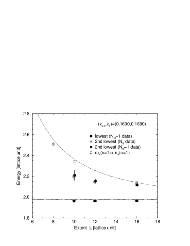
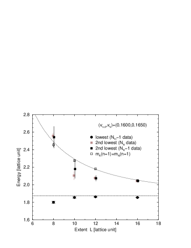
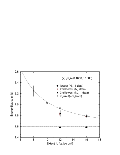
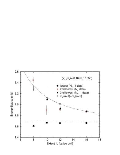
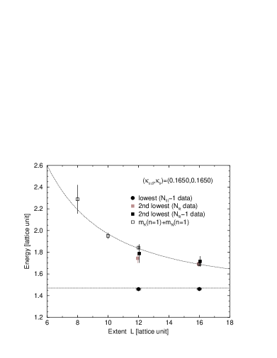
Figure 7: The black (gray) filled-squares denote the lattice QCD data of the 2nd-lowest state in $(I,J^{P})=(0,\frac{1}{2}^{-})$ channel extracted with $N_{\rm fit}-1$ ($N_{\rm fit}$) data plotted against the lattice extent $L$. The filled circles represent the lattice QCD data $E_{0}^{-}$ of the lowest state in $(I,J^{P})=(0,\frac{1}{2}^{-})$ channel. The open symbols are the sum $E_{N}^{\rm|\vec{\bf n}|=1}+E_{K}^{\rm|\vec{\bf n}|=1}$ of energies of nucleon $E_{N}^{\rm|\vec{\bf n}|=1}$ and Kaon $E_{K}^{\rm|\vec{\bf n}|=1}$ with the smallest lattice momentum $|\vec{\bf p}|=\frac{2\pi}{L}|\vec{\bf n}|=2\pi/L$. The upper line represents $\sqrt{M_{N}^{2}+|{\bf p}|^{2}}+\sqrt{M_{K}^{2}+|{\bf p}|^{2}}$ with $|{\bf p}|=2\pi/L$ the smallest relative momentum on the lattice. The lower line represent the simple sum $M_{N}+M_{K}$ of the masses of nucleon $M_{N}$ and Kaon $M_{K}$. We adopt the central values of $M_{N}$ and $M_{K}$ obtained on the largest lattice to draw the two lines.

We compare the lattice data $E_{1}^{-}$ with the expected behaviors $E_{NK}^{\rm|\vec{\bf n}|=1}$ for the 2nd-lowest NK scattering states. The filled squares in Fig. 7 denote $E_{1}^{-}$, the 2nd-lowest-state energies in this channel. The black and gray symbols are the lattice data obtained by the fits with $N_{\rm fit}-1$ and $N_{\rm fit}$ time slices, respectively (see the criterion.3 in the Sec. IV). The upper line shows the expected energy-dependence on $V$ of the 2nd-lowest NK scattering state $E_{NK}^{\rm|\vec{\bf n}|=1}\equiv\sqrt{M_{N}^{2}+(2\pi/L)^{2}}+\sqrt{M_{K}^{2}+(2\pi/L)^{2}}$ estimated with the next-smallest relative momentum between N and K, and with the masses $M_{K}$ and $M_{N}$ extracted on the $L=16$ lattices. Although the lattice QCD data $E_{1}^{-}$ and the expected lines $E_{NK}^{\rm|\vec{\bf n}|=1}$ almost coincide with each other on the $L=16$ lattices, which one may take as the characteristics of the 2nd-lowest scattering state, the data $E_{1}^{-}$ do not follow $E_{NK}^{\rm|\vec{\bf n}|=1}$ in the smaller lattices. (At the smallest lattices with $L=8$ (1.4 fm) in the physical unit, some results apparently coincide with each other again. However we consider that the volume with $L\sim 1.4$ fm is too small for the pentaquarks; it is difficult to tell which is the origin of the coincidence, uncontrollable finite volume effects of the pentaquarks or expected volume dependence of the 2nd-lowest NK scattering state.) Especially when the quarks are heavy, composite particles will be rather compact and we expect smaller finite volume effects besides those arising from the lattice momenta $\vec{\bf p}=\frac{2\pi}{L}\vec{\bf n}$. Moreover the statistical errors are also well controlled for the heavy quarks. Thus, the significant deviations in $1.5\lesssim L\lesssim 3$ fm with the combination of the heavy quarks, such as $(\kappa_{u,d},\kappa_{s})=(0.1600,0.1600)$, are reliable and the obtained states are difficult to explain as the NK scattering states.

Therefore one can understand this behavior with the view that this state is a resonance state rather than a scattering state. In fact, while the data with the lighter quarks have rather strong volume dependences which can be considered to arise due to the finite size of a resonance state, the lattice data exhibit almost no volume dependence with the combination of the heavy quarks especially in $1.5\lesssim L\lesssim 3$ fm, which can be regarded as the characteristic of resonance states.

VII The volume dependence of the spectral weight

For further confirmation, we investigate the volume dependence of the spectral weight Metal04 . As mentioned in Sec. II, the correlation function $\langle O(T)O^{\dagger}(0)\rangle$ can be expanded as $\langle O(T)O^{\dagger}(0)\rangle=\sum W_{i}e^{-E_{i}T}$. The spectral weight of the $i$-th state is defined as the coefficient $W_{i}$ corresponding to the overlap of the operator $O(t)$ with the $i$-th excited-state. The normalization conditions of the field $\psi$ and the states $|i\rangle$ give rise to the volume dependence of the weight factors $W_{i}$ in accordance with the types of the operators $O(t)$.

For example, in the case when a correlation function is constructed from a point-source and a zero-momentum point-sink, as $\sum_{\vec{\bf x}}\langle\Theta(\vec{{\bf x}},T+t_{\rm src})\overline{\Theta}(\vec{{\bf 0}},t_{\rm src})\rangle$, the weight factor $W_{i}$ takes an almost constant value if $|i\rangle$ is the resonance state where the wave function is localized. If the state $|i\rangle$ is a two-particle state, the situation is more complicated. Nevertheless if there is almost no interaction between the two particles, the weight factor is expected to be proportional to $\frac{1}{V}$. In the case when a source is a wall operator $\overline{\Theta}_{\rm wall}(t_{\rm src})$ as taken in this work, a definite volume dependence of $W_{i}$ is not known. Therefore, we re-examine the lowest state and the 2nd-lowest state in $(I,J^{P})=(0,\frac{1}{2}^{-})$ channel using the locally-smeared source $\overline{\Theta^{2}}_{\rm smear}(t_{\rm src})\equiv\sum_{{\bf\vec{x}}\in\Gamma}\overline{\Theta^{2}}({\bf\vec{x}},t_{\rm src})$ with $\Gamma\equiv{(\{0,3\},\{0,3\},\{0,3\})}$, which we introduce to partially enhance the ground-state overlap. Since smeared operators, whose typical sizes are much smaller than the total volume, can be regarded as local operators, we can discriminate the states using the locally-smeared operators as in the case of point operators. (We also investigated the weight factor using the point source. The results are consistent with those obtained using the locally-smeared one, but are rather noisy.) We adopt the hopping parameter $(\kappa_{u,d},\kappa_{s})=(0.1600,0.1600)$ and additionally employ $14^{3}\times 24$ lattice for this aim.

Figure 8: The spectral weight factors defined in Sec. VII are plotted against the lattice volume $V$. The left figure shows $W_{0}$ for the lowest state in $(I,J^{P})=(0,\frac{1}{2}^{-})$ channel and the right figure shows $W_{1}$ for the 2nd-lowest state. In the case when the weight factor $W_{i}$ for the $i$-th state $|i\rangle$ in a point-point correlator shows no volume dependence, $|i\rangle$ is likely to be a resonance state. On the contrary, when the $i$-th state $|i\rangle$ is a two-particle state, $W_{i}$ scales according to $1/V$.

We extract $W_{0}$ and $W_{1}$ using the two-exponential fit as $\sum_{\vec{\bf x}}\langle\Theta^{2}(\vec{{\bf x}},T+t_{\rm src})\overline{\Theta^{2}}_{\rm smear}(\vec{{\bf 0}},t_{\rm src})\rangle=W_{0}e^{-V_{0}T}+W_{1}e^{-V_{1}T}$. The fit with four free parameters $W_{0}$, $W_{1}$, $V_{0}$ and $V_{1}$ is however unstable and therefore we fix the exponents using the obtained values $E_{0}^{-}$ and $E_{1}^{-}$. The weight factors $W_{0}$ and $W_{1}$ are then obtained through the two-parameter fit as $\sum_{\vec{\bf x}}\langle\Theta^{2}(\vec{{\bf x}},T+t_{\rm src})\overline{\Theta^{2}}_{\rm smear}(\vec{{\bf 0}},t_{\rm src})\rangle=W_{0}e^{-E_{0}^{-}T}+W_{1}e^{-E_{1}^{-}T}$ in as large $t$ range ($T_{\rm min}\leq T+t_{\rm src}\leq T_{\rm max}$) as possible in order to avoid the contaminations of the higher excited-states than the 2nd-excited state (3rd-lowest state), which will bring about the instability of the fitted parameters. The fluctuations of $E_{0}^{-}$ and $E_{1}^{-}$ are taken into account through the Jackknife error estimation. Fig. 8 includes all the results with the various fit range as ($T_{\rm min}$,$T_{\rm max}$)= (16,18),(17,19),(18,20) to see the fit-range dependence. Though the results have some fit-range dependences, the global behaviors are almost the same among the three.

The left figure in Fig. 8 shows the weight factor $W_{0}$ of the lowest state in $(I,J^{P})=(0,\frac{1}{2}^{-})$ channel against the lattice volume $V$. We find that $W_{0}$ decreases as $V$ increases and that the dependence on $V$ is consistent with $\frac{1}{V}$, which is expected in the case of two-particle states. It is again confirmed that the lowest state in this channel is the NK scattering state with the relative momentum $|{\bf p}|=0$. Next, we plot the weight factor $W_{1}$ of the 2nd lowest state in the right figure. In this figure, almost no volume dependence against $V$ is found, which is the characteristic of the state in which the relative wave function is localized. (In Appendix, we try another prescription to estimate the volume dependences of the spectral weights, which requires no multi-exponential fit.) This result can be considered as one of the evidences of a resonance state lying slightly above the NK threshold.

To summarize this section, the volume dependence analysis of the eigenenergies and the weight factors of the 2nd-lowest state in $(I,J^{P})=(0,\frac{1}{2}^{-})$ channel suggests the existence of a resonance state. Although there remain the statistical errors and the possible finite-volume artifacts, the data can be consistently accounted for assuming the 2nd-lowest state to be different from ordinary scattering states. If the 2nd-lowest state were an ordinary scattering state, one had to assume a large systematic errors for heavier quarks which is hard to understand consistently.

VIII $(I,J^{P})=(0,\frac{1}{2}^{+})$ channel

Figure 9: The lattice QCD data in the $(I,J^{P})=(0,\frac{1}{2}^{+})$ channel are plotted against the lattice extent $L$. The solid line denotes the simple sum $M_{N^{*}}+M_{K}$ of the masses of the lowest-state negative-parity nucleon $M_{N^{*}}$ and Kaon $M_{K}$ obtained with the largest lattice.

In the same way as $(I,J^{P})=(0,\frac{1}{2}^{-})$ channel, we have attempted to diagonalize the correlation matrix in $(I,J^{P})=(0,\frac{1}{2}^{+})$ channel using the wall-sources $\overline{\Theta}_{\rm wall}(t)$ and the zero-momentum point-sinks $\sum_{\vec{\bf x}}\Theta(\vec{\bf x},t)$. In this channel, the diagonalization is rather unstable and we find only one state except for tiny contributions of possible other states. We plot the lattice data in Fig. 9. One finds that they have almost no volume dependence and that they coincide with the solid line which represents the simple sum $M_{N^{*}}+M_{K}$ of $M_{N^{*}}$ and $M_{K}$, with $M_{N^{*}}$ the mass of the ground state of the negative-parity nucleon. From this fact, the state we observe is concluded to be the $N^{*}$-$K$ scattering state with the relative momentum $|{\bf p}|=0$. It may sound strange because the p-wave state of N and K with the relative momentum $|{\bf p}|=2\pi/L$ should be lighter than the $N^{*}$-$K$ scattering state with the relative momentum $|{\bf p}|=0$; this lighter state is missing in our analysis. This failure would be due to the wall-like operator $\Theta_{\rm wall}(t)$. The fact that the wall operator $\Theta_{\rm wall}(t)$ is constructed by the spatially spread quark fields $\sum_{\vec{\bf x}}q({\rm x})$ with zero momentum may leads to the large overlaps with the NK scattering state with zero relative momentum. The relation between operators and overlap coefficients is an interesting problem and is to be explored in detail for further studies. Anyway, the strong dependence on the choice of operators suggests that it is needed to try various types of operators before giving the final conclusion.

Before closing this section, we show the spectral weight $W_{0}^{+}$ obtained by the fit using the form $\langle\Theta^{1}(t+t_{\rm src})\overline{\Theta^{1}}_{\rm wall}(t_{\rm src})\rangle=W_{0}^{+}e^{-E_{0}^{+}t}$ in Fig. 10.

Figure 10: The spectral weight factor of the extracted state in $(I,J^{P})=(0,\frac{1}{2}^{+})$ channel with the hopping parameters $(\kappa_{u,d},\kappa_{s})=(0.1600,0.1600)$ is plotted against the lattice volume $V$. We note here that the ${1}/{V}$-like volume dependence is not always the characteristics of scattering states when we do not adopt point-point correlators as is the present case. To conclude from this dependence, we need to determine the precise volume dependences of the weight factors in wall-point correlators.

Although one sees the $\frac{1}{V}$-like volume dependence in Fig. 10, one can conclude nothing only from this behavior unless the precise volume dependences of the weight factors in wall-point correlators are estimated.

IX Discussion

IX.1 Operator dependence

We here mention the operator dependences in $(I,J^{P})=(0,\frac{1}{2}^{-})$ channel. As is seen in Sec. VIII, the overlap factors with states strongly depend on the choice of operators. We survey the effective masses of the five correlators; $\sum_{\rm\vec{x}}\langle\Theta^{1}({\rm\vec{x}},T+t_{\rm src})\overline{\Theta^{1}}_{\rm wall}(t_{\rm src})\rangle$, $\sum_{\rm\vec{x}}\langle\Theta^{2}({\rm\vec{x}},T+t_{\rm src})\overline{\Theta^{2}}_{\rm wall}(t_{\rm src})\rangle$, $\sum_{\rm\vec{x}}\langle\Theta^{1}({\rm\vec{x}},T+t_{\rm src})\overline{\Theta^{1}}(t_{\rm src})\rangle$, $\sum_{\rm\vec{x}}\langle\Theta^{2}({\rm\vec{x}},T+t_{\rm src})\overline{\Theta^{2}}(t_{\rm src})\rangle$ and $\sum_{\rm\vec{x}}\langle\Theta^{3}({\rm\vec{x}},T+t_{\rm src})\overline{\Theta^{3}}(t_{\rm src})\rangle$. The effective mass E(T) is defined as a ratio between correlators with the temporal separation $T$ and $T+1$,

$$E(T)\equiv\ln\frac{\langle O(T)O(0)^{\dagger}\rangle}{\langle O(T+1)O(0)^{\dagger}\rangle},$$ (19)

which can be expressed in terms of the eigenenergies and spectral weights as

$$E(T)=\ln\frac{\sum_{i}W_{i}e^{-E_{i}T}}{\sum_{i}W_{i}e^{-E_{i}(T+1)}}\sim E_{0}+\frac{W_{1}}{W_{2}}e^{-(E_{1}-E_{0})T}+....$$ (20)

A plateau in E(T) at $E_{0}$ implies the ground-state dominance in the correlator. Effective mass plots $E(T)$ are often used to find the range where correlators show a single-exponential behavior; the higher excited-state contributions $W_{i}e^{-E_{i}T}(i>0)$ are negligible in comparison with the ground-state component $W_{0}e^{-E_{0}T}$.

Here, $\Theta^{3}$ is an interpolation operator defined as

$$\Theta^{3}(x)\equiv\varepsilon^{\rm abc}\varepsilon^{\rm aef}\varepsilon^{\rm bgh}[u_{e}(x)Cd_{f}(x)][u_{g}(x)C\gamma_{5}d_{h}(x)]C\bar{s}_{c}(x)$$ (21)

which has a di-quark structure similar to that proposed by Jaffe and Wilczek JW03 , and is also used in Refs. S03 ; IDIOOS04 ; CH04 .

Figure 11: The effective mass plots constructed from $\sum_{\rm\vec{x}}\langle\Theta^{1}({\rm\vec{x}},T+t_{\rm src})\overline{\Theta^{1}}_{\rm wall}(t_{\rm src})\rangle$, $\sum_{\rm\vec{x}}\langle\Theta^{2}({\rm\vec{x}},T+t_{\rm src})\overline{\Theta^{2}}_{\rm wall}(t_{\rm src})\rangle$, $\sum_{\rm\vec{x}}\langle\Theta^{1}({\rm\vec{x}},T+t_{\rm src})\overline{\Theta^{1}}(t_{\rm src})\rangle$, $\sum_{\rm\vec{x}}\langle\Theta^{2}({\rm\vec{x}},T+t_{\rm src})\overline{\Theta^{2}}(t_{\rm src})\rangle$ and $\sum_{\rm\vec{x}}\langle\Theta^{3}({\rm\vec{x}},T+t_{\rm src})\overline{\Theta^{3}}(t_{\rm src})\rangle$, in $(I,J^{P})=(0,\frac{1}{2}^{-})$ channel in $16^{3}\times 24$ lattice at $\beta=5.7$ employing the hopping parameters ($\kappa_{u,s},\kappa_{s}$)=(0.1600,0.1600) are plotted, along with the dashed line which denotes the lowest-state energy $E_{0}^{-}$.

Fig. 11 shows the effective mass plots constructed from $\sum_{\rm\vec{x}}\langle\Theta^{1}({\rm\vec{x}},T+t_{\rm src})\overline{\Theta^{1}}_{\rm wall}(t_{\rm src})\rangle$, $\sum_{\rm\vec{x}}\langle\Theta^{2}({\rm\vec{x}},T+t_{\rm src})\overline{\Theta^{2}}_{\rm wall}(t_{\rm src})\rangle$, $\sum_{\rm\vec{x}}\langle\Theta^{1}({\rm\vec{x}},T+t_{\rm src})\overline{\Theta^{1}}(t_{\rm src})\rangle$, $\sum_{\rm\vec{x}}\langle\Theta^{2}({\rm\vec{x}},T+t_{\rm src})\overline{\Theta^{2}}(t_{\rm src})\rangle$ and $\sum_{\rm\vec{x}}\langle\Theta^{3}({\rm\vec{x}},T+t_{\rm src})\overline{\Theta^{3}}(t_{\rm src})\rangle$. One can see two typical behaviors in the figure. One is the line damping from a large value to the energy $E_{0}^{-}$ of the lowest NK scattering state. The other is the one arising upward to $E_{0}^{-}$. Surprisingly, the differences of the spinor structure or the color structure among the operators are hardly reflected in the effective mass plots. The difference is enough to perform the variational method but seems insufficient for a clear change of the effective mass plots. Instead, the effective mass plots seem sensitive to the spatial distribution of operators. The upper three symbols are data using the point-point correlators and the lower two symbols are those from the wall-point correlators. This means the overlap factor with each state is controlled mainly by the spatial distribution rather than the internal structure of operators, except for the overall constant. The spatially smeared operators seem to have larger overlaps with the scattering state with the relative momentum $|{\bf p}|=0$. (One can find that the overlap factor of the wall operator with the observed state in $(I,J^{P})=(0,\frac{1}{2}^{+})$ in Fig. 10 is 1000 times larger than those of point operators in Fig. 8.) One often expects that the overlap with a state could be enhanced using an operator whose spinor or color structures resembles the state. We find however no such tendency in the present analysis. The insensitivity to the spinor structures may come from the fact that the KN-type operator ($\Theta^{1}$) and the di-quark type operator ($\Theta^{3}$) are directly related by a factor of $\gamma_{5}$ and a Fierz rearrangement Metal04 . Though we have no idea about the mechanism of the insensitivity to the color structure at present, this insensitivity would have some connection with the internal color-structure of $\Theta^{+}$.

The upper three data slowly damp and do not reach the lowest energy $E_{0}^{-}$ in this $T$ range, which can be explained in terms of the spectral weight. As is seen in Fig. 8, $W_{0}$ is ten-times smaller than $W_{1}$ in the case of the point-point correlator. Then, the term $\frac{W_{1}}{W_{0}}e^{-(E_{1}^{-}-E_{0}^{-})t}$ in the effective mass survives at relatively large $T$. Hence the effective mass needs larger $T$ to show a plateau at $E_{0}^{-}$. The insensitivity of the overlaps to the internal structure of operators could be helpful for us: We have adopted two operators whose color and spinor structures are different from each other. Although the difference is enough in $(I,J^{P})=(0,\frac{1}{2}^{-})$ channel, it may be insufficient in $(I,J^{P})=(0,\frac{1}{2}^{+})$ channel, which leads to the failure in the diagonalization. If we use operators with spatial distributions different from each other, it would be more effective in the diagonalization method.

IX.2 Comment on other works

Here we comment on other works previously published, especially for the pioneering works by Csikor et al. CFKK03 and Sasaki S03 . The simulation condition for the former is rather similar to ours.

Csikor et al. first reported the possible pentaquark state slightly above the NK threshold in $(I,J^{P})=(0,\frac{1}{2}^{-})$ channel in CFKK03 . In Ref. CFKK03 , they tried chiral extrapolations and taking the continuum limit at the quenched level for the possible pentaquark state. However they used the single-exponential fit analysis for the non-lowest state, namely the possible pentaquark state, for the main results. It is difficult to justify their result unless the coupling of the operators to the lowest NK state is extremely small.

Sasaki found a double-plateau in the effective mass plot and identified the 2nd-lowest plateau as the signal of $\Theta^{+}$. Unfortunately, we does not find a double-plateau in the present analysis. The double-plateau-like behavior in effective mass plots can appear only under the extreme condition that $W_{1}$ is much larger than $W_{0}$. $W_{1}$ which is ten times larger than $W_{0}$ seen in Fig. 8 and the statistical fluctuations may cause the deviation of the effective mass plot from the single monotonous line. In fact, the effective mass plot very slowly approaches $E_{0}^{-}$ as $T$ increases in Fig. 11. He extracted the mass of the next-lowest state with a single and double exponential fits. The result do not contradict with ours.

Ref. Metal04 reports a lattice QCD study which adopted the overlap-fermions with the exact chiral symmetry. The hybrid-boundary method was suggested in Ref. IDIOOS04 and the authors tried to single out the possible resonance state. In these two studies, the absence of resonance states with a mass a few hundred MeV above the NK threshold was concluded. We have not found the resonance state which coincides just with the mass of $\Theta^{+}$ in the chiral limit. In this sense, the results in Refs. Metal04 ; IDIOOS04 are not inconsistent with ours.

IX.3 chiral extrapolation

We perform chiral extrapolations for Kaon, nucleon, NK threshold (a simple sum of a Kaon mass and a nucleon mass) and the 2nd-lowest state in the $(I,J^{P})=(0,\frac{1}{2}^{-})$ channel. We adopt the lattice data with $16^{3}\times 24$ lattice, the largest lattice in our analysis. One can find in Fig. 7 that the 2nd-lowest state, which is expected to be a resonance state, is already affected by the finite volume effects for $L\leq 12$ with the lightest combination of quarks, and we therefore adopt the largest-lattice data for safety. We can expect from this fact that the typical diameter of this resonance is about 2 fm or longer and that it is desirable to use larger lattices than, $(2.5\ {\rm fm})^{3}$ for the analysis of $\Theta^{+}$.

In Fig. 12, $M_{K}+M_{N}$ and $E_{1}^{-}$ obtained with each combination of quark masses for $12^{3}\times 24$ and $16^{3}\times 24$ lattices are plotted against $m_{\pi}^{2}$. We assume the linear function of quark masses, $E_{\rm B}(m_{\rm u,d},m_{\rm s})=b_{00}+b_{10}m_{\rm u,d}+b_{01}m_{\rm s}$, for nucleon and the 2nd-lowest state with $b_{ij}$ free parameters fitted using the five lattice data. We determine the critical $\kappa$ ($\kappa_{c}$) by $M_{\pi}^{2}$ and fix the $\kappa_{s}$ so that the physical Kaon mass is reproduced in the chiral limit, using the form for pseudo scalar mesons $E^{2}_{\rm PS}(m_{\rm u,d},m_{\rm s})=a_{10}m_{\rm u,d}+a_{01}m_{\rm s}$. The chiral-extrapolated values of $M_{K}$, $M_{N}$, $M_{K}+M_{N}$ and $E_{1}^{-}$ for $16^{3}\times 24$ lattice are 0.4274(12), 0.7996(60), 1.227(6) and 1.500(52) in the lattice unit and 0.5001(14), 0.9355(70), 1.436(7) and 1.755(61) in the unit of GeV, respectively. We find that the results for $12^{3}\times 24$ lattice are consistent within errors as shown in Fig. 12.

The value of $E_{1}^{-}$=1755(61) MeV in the chiral limit is significantly larger than the mass of $\Theta^{+}(1540)$ in the real world. How can we interpret this deviation? One possibility is the systematic errors from the discretization, the chiral extrapolation, or quenching. Another possibility is that the observed 2nd-lowest state might be a signal of a resonance state lying higher than $\Theta^{+}$. Unfortunately there is no clear explanation at this point. Obviously more extensive studies on finer lattices with lighter quark masses in unquenched QCD are required. However, we can at least conclude that our quenched lattice calculations suggest the existence of a resonance-like state slightly above the NK threshold for the parameter region we have investigated.

Figure 12: A comparison of the chiral extrapolations in $(I,J^{P})=(0,\frac{1}{2}^{-})$ channel on $12^{3}\times 24$ (left) and $16^{3}\times 24$ (right) lattices for the NK threshold energy $M_{K}+M_{N}$ and the 2nd-lowest state energy $E_{1}^{-}$. $M_{K}+M_{N}$ and $E_{1}^{-}$ are plotted against $M_{\pi}^{2}$. The filled circles (triangles) denote the energies of the NK threshold (2nd-lowest state) in the chiral limit. $\kappa_{s}$ is fixed to be $\kappa_{s}\sim 0.1620$ so that the physical Kaon mass is reproduced in the chiral limit.

X Summary and Future works

We have performed the lattice QCD study of the $(S,I,J)=(+1,0,\frac{1}{2})$ states on $8^{3}\times 24$, $10^{3}\times 24$, $12^{3}\times 24$ and $16^{3}\times 24$ lattices at $\beta$=5.7 at the quenched level with the standard plaquette gauge action and Wilson quark action. To avoid the possible contaminations originating from the (anti)periodic boundary condition, which are peculiar to the pentaquark and have not been properly noticed in previous studies, we have adopted the Dirichlet boundary condition in the temporal direction for the quark field. With the aim to separate states clearly, we have adopted two independent operators with $I=0$ and $J^{P}=\frac{1}{2}$ so that we can construct a $2\times 2$ correlation matrix.

From the correlation matrix of the operators, we have successfully obtained the energies of the lowest state and the 2nd-lowest state in the $(I,J^{P})=(0,\frac{1}{2}^{-})$ channel. The volume dependence of the energies and spectral weight factors show that the 2nd-lowest state in this channel is likely to be a resonance state located slightly above the NK threshold and that the lowest state is the NK scattering state with the relative momentum $|{\bf p}|=0$. As for the $(I,J^{P})=(0,\frac{1}{2}^{+})$ channel, we have observed only one state in the present analysis, which is likely to be a $N^{*}K$ scattering state of the ground state of the negative-parity nucleon $N^{*}$ and Kaon with the relative momentum $|{\bf p}|=0$.

We have also investigated the overlaps using five independent operators. As a result, we have found that the overlaps seem to be insensitive to the spinor and color structure of operators while the overlaps are mainly controlled by the spatial distributions of operators, at least for a few low-lying state in this analysis. For the diagonalization method, it may be more effective to vary the spatial distributions rather than the internal structures.

The volume dependence of $E_{1}^{-}$ suggests that this resonance-like state in the $(I,J^{P})=(0,\frac{1}{2}^{-})$ channel is a rather spread object with the radius of about 1 fm or more. The possibility of a resonance state lying in $(I,J^{P})=(0,\frac{1}{2}^{-})$ channel is desired to be confirmed by other theoretical studies, such as quark models, QCD sum rules, string models and so on O04 ; J04 ; P03 ; EMN04 ; SDO04 ; TS04-2 ; HH05 . Unfortunately, four quarks uudd and one antiquark $\bar{s}$ in $J=\frac{1}{2}^{-}$ state can hardly reproduce the unusually narrow width of $\Theta^{+}$ so far, while the obtained mass in $J^{P}=\frac{1}{2}^{-}$ channel could be assigned to the observed resonance state TS04-2 ; HH05 . Hence, $J^{P}=\frac{3}{2}^{-}$ or $J^{P}=\frac{1}{2}^{+}$ states are favored to reproduce the width in terms of the quark model. However, there are many unknown problems left so far such as the internal structure of multi-quark hadrons J04 ; JW03 ; TMNS01 ; BKST04 ; OST04 ; AK04 or the dynamics of the string/flux-tubes BKST04 ; OST04 . The discovery of $\Theta^{+}$ gives us many challenges in the hadron physics and more detailed theoretical study including the lattice QCD studies are awaited.

For further analyses, a variational analysis using the $3\times 3$ correlation matrix or larger matrices will be desirable. The observation of wave functions will be also useful to distinguish a resonance state from scattering states and to investigate the internal structures of hadrons. We can use the lattice QCD calculations in order to estimate the decay width DDDJFMP98 and to study the flux-tube dynamics BKST04 ; OST04 ; C04 , which should give useful inputs for model calculations.

NOTE ADDED

After the completion of this paper, Refs. Letal05 ; CFKKT05 ; AT05 which also study the pentaquark state with lattice QCD have appeared on the preprint server.

($\kappa_{u,d}$,$\kappa_{s}$)=(0.1650,0.1650)

size	$M_{\pi}$	$M_{K}$	$M_{N}$	$M_{N^{*}}$	$E_{0}^{-}$	$E_{1}^{-}$	$E_{NK}$	$E_{0}^{+}$
$8^{3}\times 24$	0.4378(49)	0.4378(49)	1.0463(89)	1.4706(338)	—	—	1.3841(202)	—
$10^{3}\times 24$	0.4543(17)	0.4543(17)	1.0591(91)	1.4313(292)	—	—	1.4704(202)	2.0987(45)
$12^{3}\times 24$	0.4563(13)	0.4563(13)	1.0281(74)	1.4760(309)	1.4601( 75)	1.7881(829)	1.4715(107)	2.0502(26)
$16^{3}\times 24$	0.4556(11)	0.4556(11)	1.0143(44)	1.4791(278)	1.4616( 56)	1.7157(452)	1.4743( 74)	1.9951(19)

($\kappa_{u,d}$,$\kappa_{s}$)=(0.1625,0.1650)

size	$M_{\pi}$	$M_{K}$	$M_{N}$	$M_{N^{*}}$	$E_{0}^{-}$	$E_{1}^{-}$	$E_{NK}$	$E_{0}^{+}$
$8^{3}\times 24$	0.5747(21)	0.5130(31)	1.2112(133)	1.5973(220)	1.6123(139)	2.6447(3322)	1.6119(195)	2.2065(368)
$10^{3}\times 24$	0.5785(11)	0.5199(14)	1.1814( 55)	1.5712( 93)	1.6673( 96)	2.0912(2305)	1.6687(127)	2.2120(393)
$12^{3}\times 24$	0.5792(10)	0.5205(10)	1.1655( 47)	1.5930(175)	1.6612( 55)	1.9228(348)	1.6763( 70)	2.2145(293)
$16^{3}\times 24$	0.5789( 9)	0.5209(10)	1.1590( 37)	1.5888(169)	1.6636( 42)	1.8769(225)	1.6745( 50)	2.1734(223)

($\kappa_{u,d}$,$\kappa_{s}$)=(0.1600,0.1650)

size	$M_{\pi}$	$M_{K}$	$M_{N}$	$M_{N^{*}}$	$E_{0}^{-}$	$E_{1}^{-}$	$E_{NK}$	$E_{0}^{+}$
$8^{3}\times 24$	0.6839(18)	0.5761(25)	1.3270(110)	1.6956( 54)	1.8002(121)	2.5420(1226)	1.8109(259)	2.3666(122)
$10^{3}\times 24$	0.6873(10)	0.5819(12)	1.3070( 48)	1.6810(131)	1.8549( 78)	2.1797(1067)	1.8574( 90)	2.3547(253)
$12^{3}\times 24$	0.6883( 9)	0.5816(11)	1.3003( 48)	1.7198(221)	1.8627( 51)	2.0736(306)	1.8680( 57)	2.4004(396)
$16^{3}\times 24$	0.6867( 9)	0.5818( 9)	1.2921( 30)	1.7193(222)	1.8546( 37)	2.0429(156)	1.8668( 42)	2.3403(162)

($\kappa_{u,d}$,$\kappa_{s}$)=(0.1650,0.1600)

size	$M_{\pi}$	$M_{K}$	$M_{N}$	$M_{N^{*}}$	$E_{0}^{-}$	$E_{1}^{-}$	$E_{NK}$	$E_{0}^{+}$
$8^{3}\times 24$	0.4378(49)	0.5761(25)	1.0463( 89)	1.4705(338)	—	—	1.5150(259)	2.0510(732)
$10^{3}\times 24$	0.4543(17)	0.5823(17)	1.0774(128)	1.4313(292)	—	—	1.6088(173)	2.1897(1549)
$12^{3}\times 24$	0.4563(13)	0.5816(11)	1.0281( 74)	1.4760(309)	1.5838( 72)	1.8368(538)	1.5951(100)	2.1645(440)
$16^{3}\times 24$	0.4556(11)	0.5818( 9)	1.0143( 44)	1.4791(278)	1.5852( 55)	1.7855(313)	1.5987( 73)	2.0823(176)

($\kappa_{u,d}$,$\kappa_{s}$)=(0.1600,0.1600)

size	$M_{\pi}$	$M_{K}$	$M_{N}$	$M_{N^{*}}$	$E_{0}^{-}$	$E_{1}^{-}$	$E_{NK}$	$E_{0}^{+}$
$8^{3}\times 24$	0.6839(18)	0.6839(18)	1.3270(110)	1.6956( 54)	—	—	1.9239(226)	2.4376(105)
$10^{3}\times 24$	0.6873(10)	0.6873(10)	1.3070( 48)	1.6810(131)	1.9622( 73)	2.2085(478)	1.9617( 87)	2.4319(215)
$12^{3}\times 24$	0.6883( 9)	0.6883( 9)	1.2987( 42)	1.7198(221)	1.9632( 51)	2.1528(195)	1.9705( 56)	2.4820(312)
$16^{3}\times 24$	0.6867( 9)	0.6867( 9)	1.2906( 30)	1.7193(222)	1.9641( 40)	2.1158(153)	1.9723( 41)	2.4180(138)

Table 1: The pion masses $M_{\pi}$, Kaon masses $M_{K}$, nucleon masses $M_{N}$, masses of the ground state of negative-parity nucleon $M_{N^{*}}$, energies of the lowest state $E_{0}^{-}$, energies of the 2nd-lowest state $E_{1}^{-}$, energies of the lowest state $E_{NK}$ (obtained by single-exponential fit) in the $(I,J^{P})=(0,\frac{1}{2}^{-})$ channel are listed. The energies of the obtained state $E_{0}^{+}$ in the $(I,J^{P})=(0,\frac{1}{2}^{+})$ channel are also listed. $\kappa_{u,d}$ and $\kappa_{s}$ are the hopping parameters for $u,d$ quarks and $s$ quark respectively.

Appendix A additional estimations of weight factors

In this appendix, we make another trial to estimate volume dependences of weight factors in $(I,J^{P})=(0,\frac{1}{2}^{-})$ channel. As seen in Sec. VII, we have extracted the weight factors using double-exponential fit, which is however rather unstable and we have therefore fixed the exponents. We here discuss the possibility of methods without any multi-exponential fits. Let us again consider $N\times N$ correlation matrices constructed by $\gamma$-sink $\alpha$-source and $\gamma$-sink $\beta$-source correlators. Here $\alpha,\beta,\gamma$ denote the types of operators, such as “point” or “wall” or “smear” and so on. The notations are the same as those in Sec. II. The $\gamma-\alpha$ and $\gamma-\beta$ correlation matrices are described as

$${\cal C}_{IJ}^{\rm\gamma\alpha}(T)\equiv\langle{\Theta}^{I}_{\gamma}(T+t_{\rm src})\overline{{\Theta}^{J}_{\alpha}}(t_{\rm src})\rangle=(C^{\gamma\dagger}\Lambda(T)C^{\alpha})_{IJ}+d_{IJ}e^{-E_{N}T}+...$$ (22)

$${\cal C}_{IJ}^{\rm\gamma\beta}(T)\equiv\langle{\Theta}^{I}_{\gamma}(T+t_{\rm src})\overline{{\Theta}^{J}_{\beta}}(t_{\rm src})\rangle=(C^{\gamma\dagger}\Lambda(T)C^{\beta})_{IJ}+d^{\prime}_{IJ}e^{-E_{N}T}+...$$ (23)

with $N\times N$ matrices ($d_{IJ}e^{-E_{N}T}+...$) and ($d^{\prime}_{IJ}e^{-E_{N}T}+...$) being possible higher excited-state contaminations. We hereby consider two quantities; $\left[{\cal C}_{IJ}^{\rm\gamma\alpha}(T){\cal C}_{IJ}^{\rm\gamma\alpha}(T+1)^{-1}\right]^{T}{\cal C}_{IJ}^{\rm\gamma\alpha}(T)$ defined using one type of the correlation matrix and $[{\cal C}_{IJ}^{\rm\gamma\alpha}(T)]^{-1}{\cal C}_{IJ}^{\rm\gamma\beta}(T)$, which with large $T$ lead to

$$\left[{\cal C}_{IJ}^{\rm\gamma\alpha}(T){\cal C}_{IJ}^{\rm\gamma\alpha}(T+1)^{-1}\right]^{T}{\cal C}_{IJ}^{\rm\gamma\alpha}(T)=C^{\gamma\dagger}C^{\alpha}+{\cal F}(D(T))+....$$ (24)

and

$$[{\cal C}_{IJ}^{\rm\gamma\alpha}(T)]^{-1}{\cal C}_{IJ}^{\rm\gamma\beta}(T)=(C^{\alpha})^{-1}C^{\beta}+{\cal F}^{\prime}(D(T))+...,$$ (25)

respectively. Here ${\cal F}(D(T))$ and ${\cal F}^{\prime}(D(T))$ are terms including $N\times N$ diagonal matrix $D(T)\equiv{\rm diag}(e^{-(E_{N}-E_{N-1})T},...,e^{-(E_{N}-E_{0})T})$. Then, each component of $\left[{\cal C}_{IJ}^{\rm\gamma\alpha}(T){\cal C}_{IJ}^{\rm\gamma\alpha}(T+1)^{-1}\right]^{T}{\cal C}_{IJ}^{\rm\gamma\alpha}(T)$ and $[{\cal C}_{IJ}^{\rm\gamma\alpha}(T)]^{-1}{\cal C}_{IJ}^{\rm\gamma\beta}(T)$ gets stable and shows a plateau in large $T$ region, where ${\cal F}(D(T))$ and ${\cal F}^{\prime}(D(T))$ are negligible.

Next, we relate these quantities to spectral weights. For this aim, we simply take the determinants. In the case when the correlation matrices are $2\times 2$ matrices, the determinant $\det\left((C^{\alpha})^{-1}C^{\beta}\right)$ is explicitly written as $\det C^{\beta}/\det C^{\alpha}=\varepsilon^{IJ}C^{\beta}_{0I}C^{\beta}_{1J}/\varepsilon^{I^{\prime}J^{\prime}}C^{\alpha}_{0I^{\prime}}C^{\alpha}_{1J^{\prime}}$, and the determinant $\det\left(C^{\gamma\dagger}C^{\beta}\right)$ is expressed as $(\det C^{\gamma\dagger})\times(\det C^{\beta})=(\varepsilon^{IJ}C^{\gamma\dagger}_{I0}C^{\gamma\dagger}_{J1})\times(\varepsilon^{I^{\prime}j^{\prime}}C^{\beta}_{0I^{\prime}}C^{\beta}_{1J^{\prime}})=\varepsilon^{IJ}\varepsilon^{I^{\prime}J^{\prime}}C^{\gamma\dagger}_{I0}C^{\beta}_{0I^{\prime}}C^{\gamma\dagger}_{J1}C^{\beta}_{1J^{\prime}}$. The term $C^{\beta}_{0I}C^{\beta}_{1J}$ ($C^{\alpha}_{0I}C^{\alpha}_{1J}$) denotes the product of the overlaps of the $\beta$($\alpha$)-type operator with the lowest state and the 2nd-lowest state. On the other hand, $C^{\gamma\dagger}_{I0}C^{\beta}_{0I^{\prime}}$ ($C^{\gamma\dagger}_{J1}C^{\beta}_{1J^{\prime}}$) corresponds to the spectral weight for the lowest (2nd-lowest) state in the $\beta$-$\gamma$ correlator in terms of a volume dependence.

Let us consider the several cases when ($\alpha,\beta,\gamma$)={W(wall), S(smeared), P(point)}. The term $\det(C^{{\rm P}\dagger}C^{\rm S})$ behaves showing the same volume dependence as the product of the spectral weights for the lowest and the 2nd-lowest state in the smeared-point correlator, which should be $\sim\frac{1}{V}\times 1=\frac{1}{V}$ if the lowest state is a scattering state and the 2nd-lowest state is a resonance state. The left panel in Fig. 13 represents $\det\left(\left[{\cal C}_{IJ}^{\rm PS}(T){\cal C}_{IJ}^{\rm PS}(T+1)^{-1}\right]^{T}{\cal C}_{IJ}^{\rm PS}(T)\right)$ on each volume. However, $\det\left(\left[{\cal C}_{IJ}^{\rm PS}(T){\cal C}_{IJ}^{\rm PS}(T+1)^{-1}\right]^{T}{\cal C}_{IJ}^{\rm PS}(T)\right)$ on each volume, which approaches $\det(C^{{\rm P}\dagger}C^{\rm S})$ with large $T$, has relatively large errors and fluctuations with no clear plateau and we fail to extract $\det(C^{{\rm P}\dagger}C^{\rm S})$. This would be due to the smallness of the signals in smeared-point correlators. Meanwhile, $\det\left(\left[{\cal C}_{IJ}^{\rm PW}(T){\cal C}_{IJ}^{\rm PW}(T+1)^{-1}\right]^{T}{\cal C}_{IJ}^{\rm PW}(T)\right)$ shown in the middle panel in Fig. 13 and $\det\left([{\cal C}_{IJ}^{\rm PW}(T)]^{-1}{\cal C}_{IJ}^{\rm PS}(T)\right)$ shown in the right panel in Fig. 13, which approach $\det(C^{{\rm P}\dagger}C^{\rm W})$ and $\det((C^{\rm W})^{-1}C^{\rm S})$ respectively, show relatively clear plateaus. Therefore we extract $\det(C^{{\rm P}\dagger}C^{\rm W})$ and $\det((C^{\rm W})^{-1}C^{\rm S})$ by the fits $\det(C^{{\rm P}\dagger}C^{\rm W})=\det\left(\left[{\cal C}_{IJ}^{\rm PW}(T){\cal C}_{IJ}^{\rm PW}(T+1)^{-1}\right]^{T}{\cal C}_{IJ}^{\rm PW}(T)\right)$ and $\det((C^{\rm W})^{-1}C^{\rm S})=\det\left([{\cal C}_{IJ}^{\rm PW}(T)]^{-1}{\cal C}_{IJ}^{\rm PS}(T)\right)$ in the $T$ range where they show plateaus and we finally obtain $\det(C^{{\rm P}\dagger}C^{\rm S})$ as $\det(C^{{\rm P}\dagger}C^{\rm S})=\det(C^{{\rm P}\dagger}C^{\rm W})\times\det((C^{\rm W})^{-1}C^{\rm S})$. In Fig. 14, we show $\det(C^{{\rm P}\dagger}C^{\rm S})$ obtained by the prescription shown above. The solid line denotes the best-fit curve by $A_{1}/V$ and the dashed line does the best-fit curve by $A_{2}/V^{2}$. The best fit parameters are $A_{1}=1.35$ and $A_{2}=2.17$, and $\chi^{2}/N_{\rm df}$ is 1.72 and 7.13 respectively. The volume dependence of $\det(C^{{\rm P}\dagger}C^{\rm S})$ seems not to be inconsistent with $\frac{1}{V}$. If we know the precise volume dependence of overlaps of wall operators, we may be discriminate the states using $\det(C^{{\rm P}\dagger}C^{\rm W})$ or $\det((C^{\rm W})^{-1}C^{\rm S})$.

Figure 13: The left figure shows $\det\left(\left[{\cal C}_{IJ}^{\rm PS}(T){\cal C}_{IJ}^{\rm PS}(T+1)^{-1}\right]^{T}{\cal C}_{IJ}^{\rm PS}(T)\right)$ as the function of $T$ on each volume. The middle figure is the plot of $\det\left(\left[{\cal C}_{IJ}^{\rm PW}(T){\cal C}_{IJ}^{\rm PW}(T+1)^{-1}\right]^{T}{\cal C}_{IJ}^{\rm PW}(T)\right)$ against $T$. ${\rm Det}\left([{\cal C}_{IJ}^{\rm PW}(T)]^{-1}{\cal C}_{IJ}^{\rm PS}(T)\right)$ is plotted in the right figure. ${\rm Det}\left(\left[{\cal C}_{IJ}^{\rm PS}(T){\cal C}_{IJ}^{\rm PS}(T+1)^{-1}\right]^{T}{\cal C}_{IJ}^{\rm PS}(T)\right)$, $\det\left(\left[{\cal C}_{IJ}^{\rm PW}(T){\cal C}_{IJ}^{\rm PW}(T+1)^{-1}\right]^{T}{\cal C}_{IJ}^{\rm PW}(T)\right)$ and $\det\left([{\cal C}_{IJ}^{\rm PW}(T)]^{-1}{\cal C}_{IJ}^{\rm PS}(T)\right)$ show plateaus in the large $T$ region and coincide with $\det(C^{{\rm P}\dagger}C^{\rm S})$, $\det(C^{{\rm P}\dagger}C^{\rm W})$ and $\det((C^{\rm W})^{-1}C^{\rm S})$ respectively.

Figure 14: ${\rm Det}(C^{{\rm P}\dagger}C^{\rm S})$ is plotted as the function of the lattice volume $V$. The solid line denotes the best-fit curve by $A_{1}/V$ and the dashed line does the best-fit curve by $A_{2}/V^{2}$. The best fit parameters are $A_{1}=1.35$ and $A_{2}=2.17$, and $\chi^{2}/N_{\rm df}$ is 1.72 and 7.13 respectively. These data behaves consistently in accordance with $1/V$.

References

• (1) T.Β Nakano et al. [LEPS Collaboration], Phys.Β Rev.Β Lett.Β  91, 012002 (2003) [arXiv:hep-ex/0301020].
• (2) V.Β V.Β Barmin et al. [DIANA Collaboration], Phys.Β Atom.Β Nucl.Β  66, 1715 (2003) [Yad.Β Fiz.Β  66, 1763 (2003)] [arXiv:hep-ex/0304040].
• (3) S.Β Stepanyan et al. [CLAS Collaboration], Phys.Β Rev.Β Lett.Β  91, 252001 (2003) [arXiv:hep-ex/0307018].
• (4) J.Β Barth et al. [SAPHIR Collaboration], Phys.Β Lett.Β B 572, 127 (2003).
• (5) S.Β Chekanov et al. [ZEUS Collaboration], Phys.Β Lett.Β B 591, 7 (2004) [arXiv:hep-ex/0403051].
• (6) A.Β E.Β Asratyan, A.Β G.Β Dolgolenko and M.Β A.Β Kubantsev, Phys.Β Atom.Β Nucl.Β  67, 682 (2004) [Yad.Β Fiz.Β  67, 704 (2004)] [arXiv:hep-ex/0309042].
• (7) A.Β Airapetian et al. [HERMES Collaboration], Phys.Β Lett.Β B 585, 213 (2004) [arXiv:hep-ex/0312044].
• (8) M.Β Abdel-Bary et al. [COSY-TOF Collaboration], Phys.Β Lett.Β B 595, 127 (2004) [arXiv:hep-ex/0403011].
• (9) V.Β Kubarovsky et al. [CLAS Collaboration], Phys.Β Rev.Β Lett.Β  92, 032001 (2004) [Erratum-ibid.Β  92, 049902 (2004)] [arXiv:hep-ex/0311046].
• (10) M.Β Oka, Prog.Β Theor.Β Phys.Β  112, 1 (2004) and references therein [arXiv:hep-ph/0406211].
• (11) R.Β L.Β Jaffe, Phys.Β Rept.Β  409, 1 (2005) [Nucl.Β Phys.Β Proc.Β Suppl.Β  142, 343 (2005)] [arXiv:hep-ph/0409065].
• (12) D. Diakonov, V. Petrov and M. Polyakov, Z. Phys. A 359, 305 (1997).
• (13) M.Β Praszalowicz, Phys.Β Lett.Β B 575, 234 (2003) [arXiv:hep-ph/0308114].
• (14) Fl. Stancu and D. O. Riska, Phys. Lett. B575, 242 (2003) [arXiv:hep-ph/0307010];
C. E. Carlson, C.D. Carone, H.J. Kwee and V. Nazaryan, Phys. Lett. B579, 52 (2004)[arXiv:hep-ph/0310038];
Y.Β Kanada-Enyo, O.Β Morimatsu and T.Β Nishikawa, arXiv:hep-ph/0404144.
S. Takeuchi and K. Shimizu, arXiv:hep-ph/0411016.
• (15) A. Hosaka, Phys. Lett. B571, 55 (2003) [arXiv:hep-ph/0307232].
• (16) J.Β Sugiyama, T.Β Doi and M.Β Oka, Phys.Β Lett.Β B 581, 167 (2004) [arXiv:hep-ph/0309271];
T. Nishikawa, Y. Kanada-En’yo, O. Morimatsu and Y Kondo, Phys. Rev. D71, 016001 (2005)[arXiv:hep-ph/0410394];
R. D. Matheus and S. Narison, arXiv:hep-ph/0412063.
• (17) For instance, A.Β Ali Khan et al. [CP-PACS Collaboration], Phys.Β Rev.Β D 65, 054505 (2002) [Erratum-ibid.Β D 67, 059901 (2003)] [arXiv:hep-lat/0105015].
• (18) F.Β Csikor, Z.Β Fodor, S.Β D.Β Katz and T.Β G.Β Kovacs, JHEP 0311, 070 (2003) [arXiv:hep-lat/0309090].
• (19) S.Β Sasaki, Phys.Β Rev.Β Lett.Β  93, 152001 (2004) [arXiv:hep-lat/0310014].
• (20) T.Β T.Β Takahashi, T.Β Umeda, T.Β Onogi and T.Β Kunihiro, arXiv:hep-lat/0410025.
• (21) T.Β W.Β Chiu and T.Β H.Β Hsieh, arXiv:hep-ph/0403020.
• (22) N.Β Mathur et al., Phys.Β Rev.Β D 70, 074508 (2004) [arXiv:hep-ph/0406196].
• (23) N.Β Ishii, T.Β Doi, H.Β Iida, M.Β Oka, F.Β Okiharu and H.Β Suganuma, Phys.Β Rev.Β D 71, 034001 (2005) [arXiv:hep-lat/0408030].
• (24) N.Β Mathur et al., Phys.Β Lett.Β B 605, 137 (2005) [arXiv:hep-ph/0306199].
• (25) S.Β Perantonis and C.Β Michael, Nucl.Β Phys.Β B 347, 854 (1990).
• (26) M.Β Luscher and U.Β Wolff, Nucl.Β Phys.Β B 339, 222 (1990).
• (27) T.Β T.Β Takahashi and H.Β Suganuma, Phys.Β Rev.Β Lett.Β  90, 182001 (2003) [arXiv:hep-lat/0210024]; Phys.Β Rev.Β D 70, 074506 (2004) and references therein [arXiv:hep-lat/0409105].
• (28) F.Β Butler, H.Β Chen, J.Β Sexton, A.Β Vaccarino and D.Β Weingarten, Nucl.Β Phys.Β B 430, 179 (1994) [arXiv:hep-lat/9405003].
• (29) T.Β Yamazaki et al. [CP-PACS Collaboration], Phys.Β Rev.Β D 70, 074513 (2004) [arXiv:hep-lat/0402025].
• (30) M.Β Fukugita, Y.Β Kuramashi, M.Β Okawa, H.Β Mino and A.Β Ukawa, Phys.Β Rev.Β D 52, 3003 (1995) [arXiv:hep-lat/9501024].
• (31) K.Β Sasaki and S.Β Sasaki, arXiv:hep-lat/0503026.
• (32) O.Β Dumbrajs, R.Β Koch, H.Β Pilkuhn, G.Β c.Β Oades, H.Β Behrens, J.Β j.Β De Swart and P.Β Kroll, Nucl.Β Phys.Β B 216 (1983) 277.
• (33) M.Β M.Β Nagels et al., Nucl.Β Phys.Β B 147 (1979) 189.
• (34) M.Β LΓΌscher, Nucl.Β Phys.Β B 354, 531 (1991).
• (35) J.Β S.Β Hyslop, R.Β A.Β Arndt, L.Β D.Β Roper and R.Β L.Β Workman, Phys.Β Rev.Β D 46, 961 (1992).
• (36) R.Β L.Β Jaffe and F.Β Wilczek, Phys.Β Rev.Β Lett.Β  91, 232003 (2003) [arXiv:hep-ph/0307341].
• (37) S.Β Takeuchi and K.Β Shimizu, arXiv:hep-ph/0411016.
• (38) T.Β Hyodo and A.Β Hosaka, arXiv:hep-ph/0502093.
• (39) T.Β T.Β Takahashi, H.Β Matsufuru, Y.Β Nemoto and H.Β Suganuma, Phys.Β Rev.Β Lett.Β  86, 18 (2001) [arXiv:hep-lat/0006005]; T.Β T.Β Takahashi, H.Β Suganuma, Y.Β Nemoto and H.Β Matsufuru, Phys.Β Rev.Β D 65, 114509 (2002) [arXiv:hep-lat/0204011].
• (40) M.Β Bando, T.Β Kugo, A.Β Sugamoto and S.Β Terunuma, Prog.Β Theor.Β Phys.Β  112, 325 (2004) [arXiv:hep-ph/0405259].
• (41) C.Β Alexandrou and G.Β Koutsou, Phys.Β Rev.Β D 71, 014504 (2005) [arXiv:hep-lat/0407005].
• (42) F.Β Okiharu, H.Β Suganuma and T.Β T.Β Takahashi, arXiv:hep-lat/0407001; arXiv:hep-lat/0410021; arXiv:hep-lat/0412012.
• (43) G.Β M.Β de Divitiis, L.Β Del Debbio, M.Β Di Pierro, J.Β M.Β Flynn, C.Β Michael and J.Β Peisa [UKQCD Collaboration], JHEP 9810, 010 (1998) [arXiv:hep-lat/9807032].
• (44) J.Β M.Β Cornwall, arXiv:hep-ph/0412201.
• (45) B.Β G.Β Lasscock et al., arXiv:hep-lat/0503008.
• (46) F.Β Csikor, Z.Β Fodor, S.Β D.Β Katz, T.Β G.Β Kovacs and B.Β C.Β Toth, arXiv:hep-lat/0503012.
• (47) C.Β Alexandrou and A.Β Tsapalis, arXiv:hep-lat/0503013.
($\kappa_{u,d}$,ΞΊssubscriptπœ…π‘ \kappa_{s})=(0.1650,0.1650)