Calorons in $SU(3)$ lattice gauge theory

Abstract

We examine the semiclassical content of $SU(3)$ Yang Mills theory on the lattice at finite temperature. Employing the cooling method, a set of classical fields is generated from a Monte Carlo ensemble. Various operators are used to inspect this set with respect to topological properties. We find pseudoparticle fields, so-called caloron solutions, possessing the remarkable features of (superpositions of) Kraan-van Baal solutions, i.e. extensions of Harrington-Shepard calorons to generic values of the holonomy.

I Introduction

Guided by the idea that the semiclassical approach to QCD ’t Hooft (1976); Callan et al. (1978); Coleman (1977) provides a reasonable model for the QCD vacuum, one first has to specify the basic set of classical solutions of the underlying Yang-Mills theory. Mathematical rich and interesting structures naturally arise in the construction and topological classification of these fields. For $SU(N)$ gauge theory in the Euclidean space $\mathbb{R}^{4}$ solutions with finite action are the well known BPST instantons Belavin et al. (1975) and their generalizations to arbitrary topological charge Atiyah et al. (1978). The vigorous work pursuing the semiclassical approach culminated in the so-called instanton-liquid model Ilgenfritz and Müller-Preussker (1981); Shuryak (1982); Diakonov and Petrov (1984), which successfully realizes fundamental non-perturbative properties of QCD such as the $U(1)_{A}$ anomaly and chiral symmetry breaking. It has led to numerous phenomenological applications (for newer reviews see Schäfer and Shuryak (1998); Diakonov (2003)). However, it failed to reproduce one essential feature of QCD – confinement.

In case of the $SU(N)$ gauge theory with finite temperature defined on $S^{1}\times\mathbb{R}^{3}$ quark (de)confinement is closely related to the global center symmetry. The Polyakov loop at temperature $~{}T~{}$

$${\mathcal{P}}(\vec{x})={\rm P}\exp\left(\int_{0}^{b=1/T}\!\!\!A_{0}(x_{0},\vec{x})\,dx_{0}\right)\;,$$ (1)

an order parameter of this symmetry, signals a phase transition from a deconfining to a confining phase. Deconfinement is a feature of the high temperature phase, where the symmetry is spontaneously broken and – in the limit of large temperatures – the Polyakov loop takes values in the center of the gauge group $~{}Z(N)$. Below the critical temperature the symmetry becomes restored, the trace of the Polyakov loop fluctuates around zero and confinement is observed. One can hope that not only for temperatures above the transition temperature the semiclassical approach is justified. Then it should be able to reflect the transition as an important feature of the finite temperature gauge theory.

A semiclassical model for non-zero temperature QCD has first been formulated in Gross et al. (1981) starting from Harrington-Shepard (HS) caloron solutions Harrington and Shepard (1978) which represent infinite chains of time-periodic instanton solutions in $\mathbb{R}^{4}$. Restricted to the strip $S^{1}\times\mathbb{R}^{3}$ HS calorons have an integer-valued topological charge $Q_{\textnormal{t}}\in\mathbb{Z}$ like BPST instantons. For $SU(N)$ HS calorons are realized as $SU(2)$ embeddings. More restrictive from our point of view is the fact that their vector potentials behave asymptotically such that trivial holonomy emerges, i.e. their asymptotic Polyakov loop values belong to the center of the group

$${\mathcal{P}_{\infty}}\equiv\lim_{|\vec{x}|\to\infty}{\mathcal{P}}(\vec{x})\in Z(N)\,.$$ (2)

If one would have to describe only the deconfinement phase, this asymptotic behavior which is directly related to the broken center symmetry values of the order parameter is certainly adequate. Is this the case also for the confinement phase ? The authors of Gross et al. (1981) have argued that the path integral evaluated in the infinite volume limit cannot be dominated by classical fields having a non-trivial holonomy. But this conclusion does not hold for a single topological excitation created in a finite box or in the case of a finite density of such objects. Therefore, the question arises, whether there are also classical fields asymptotically matching to a vanishing order parameter as required in the confinement phase. Indeed, selfdual time-periodic caloron solutions of the $SU(N)$ Yang-Mills equations with arbitrary (non-trivial) holonomy have been explicitly constructed by Kraan and van Baal Kraan and van Baal (1998a), and Lee and Lu Lee and Lu (1998) several years ago. The new $SU(N)$ calorons – we call them KvB calorons – with integer-valued topological charge $~{}Q_{\textnormal{t}}~{}$ consist of $~{}N~{}|Q_{\textnormal{t}}|~{}$ constituents, which appear as static BPS monopoles Prasad and Sommerfield (1975); Bogomol’nyi (1976) if sufficiently separated. Their masses $8\pi^{2}~{}T~{}\nu_{m}$ are then determined by the differences of holonomy eigenvalues $\nu_{m}=\mu_{m+1}-\mu_{m}\,,$

$${\mathcal{P}_{\infty}}=g\;\exp(2\pi i\;{\rm diag}(\mu_{1},\mu_{2},\ldots,\mu_{N}))\;g^{\dagger}$$ (3)

ordered such that $~{}\mu_{1}<\mu_{2}<\cdots<\mu_{N+1}\equiv 1+\mu_{1}~{}$ and $~{}\mu_{1}+\mu_{2}+\cdots+\mu_{N}=0$. The separated and massive caloron constituents can be localized by one or more of the following criteria van Baal (2002):

1. at the centers of their three-dimensional spherical lumps of action or topological charge,

2. at the positions, where the zero-mode density of the Dirac operator in the background of the caloron field $\not{D}=\gamma^{\mu}(\partial_{\mu}+A_{\mu}^{\mathrm{caloron}})$ is maximal, depending on the temporal boundary condition for the fermion field,

3. at the points $\vec{x}$, where at least two of the eigenvalues of ${\mathcal{P}}(\vec{x})$ coincide,

4. at the positions of static Abelian (anti)monopoles representing defects of an appropriately chosen Abelian gauge.

However, if the constituents are close to each other or if they become even massless, these criteria do not hold unambiguously. The first two criteria cannot distinguish between the constituents at all. The constituents form joint non-static caloron lumps of topological charge. The last two criteria are still working, but the extracted positions will not completely agree.

In any case, the non-trivial holonomy suggests a proper link between the classical background field and the dynamics of the order parameter. Therefore, a semiclassical (variational) approach to Yang-Mills theory should be based on the new, KvB calorons. That such an approach is promising has been recently argued by Diakonov Diakonov (2003). He and his collaborators have shown that the quantum amplitude in the background of KvB calorons leads to interactions of the monopole constituents at the quantum level Diakonov et al. (2004); Diakonov (2004). These interactions become attractive at higher temperature (i.e. deconfinement) and repulsive at lower temperature (confinement). Thus, in the deconfinement phase HS calorons might be favored (with all but one constituent massless, i.e. invisible), whereas in the confinement case the repulsive interactions support a view of a gas to be described fully in terms of monopoles or KvB caloron constituents. The calculation of the fluctuation determinant still awaits extension from the $SU(2)$ case Diakonov et al. (2004); Diakonov (2004) to arbitrary $N$. The zero-mode contribution to the semiclassical integration measure can be obtained for arbitrary $N$ from the determinant of the explicit moduli space metric as computed by Kraan a few years ago Kraan (2000). This, as well as a more detailed analysis of how in particular the parameters of the $N$ monopole constituents are related to the scale parameter of the standard $SU(N)$ instanton, can be found in Ref. Diakonov and Gromov (2005).

In recent papers Ilgenfritz et al. (2002, 2004) published together with Martemyanov, Shcheredin and Veselov we have explored the existence of KvB calorons in the (simpler) case of $SU(2)$ lattice gauge theory. We first relied on the cooling method in order to search for (approximate) solutions of the Yang-Mills equations of motion. Later on we have investigated smoothed configurations obtained by four-dimensional smearing i.e. “keeping closer” to equilibrium fields Ilgenfritz et al. (2005). In both cases, starting from Monte Carlo equilibrium fields generated within the confinement phase we have shown that non-trivial holonomy with ${\rm tr}\,{\mathcal{P}}_{\infty}\simeq 0~{}$ dominates the vacuum structure. The topological lumps we have found were typically composed of monopole constituents and possessed all properties of KvB solutions (or their constituents).

In this paper we are extending our investigations to the $SU(3)$ case of finite temperature lattice gauge fields in the confinement phase. Relying on the cooling procedure our aim is again to explore the structure of (semi)classical fields at the level of a few instanton actions $~{}S=n~{}S_{\textnormal{inst}},~{}n=1,\ldots,4$ with $S_{\textnormal{inst}}=8\pi^{2}/g^{2}$. For this we had to refine our methods and to improve lattice observables. Our paper is organized as follows. In Section II we review known analytical formulae for the $SU(3)$ KvB caloron. Later on, in Section III, we describe the observables and the methods which are used to compare the analytical results with the classical lattice gauge fields. Results for typical examples of cooled lowest-action (classical) fields are presented in Section IV. The results obtained for ensembles of classical fields extracted also at higher action level are discussed in Section V.

II Properties of KvB calorons

Most analytical efforts are currently directed to improving the knowledge of higher charge $SU(2)$ calorons Bruckmann et al. (2004a). Expressions are known for topological charge-one calorons in $SU(2)$ Kraan and van Baal (1998b) and for generic $SU(N)$ Kraan and van Baal (1998c). We recall the expressions of the action $~{}s(x)~{}$ and the density of the fermionic zero-mode $~{}\Psi_{z}^{\dagger}\Psi_{z}(x)~{}$ of the $SU(3)$ single-caloron field $~{}A_{\mu}~{}$ with $~{}|Q_{\textnormal{t}}|=1~{}$. The zero-mode depends on the temporal boundary condition imposed, $~{}\Psi_{z}(x_{0}+b,\vec{x})=e^{-2\pi iz}\Psi_{z}(x_{0},\vec{x})$ (with $b=1/T$).

$$s(x) = -\frac{1}{2}\,\partial^{2}\partial^{2}\ln\psi(x_{0},\vec{x})$$ (4)

$$\Psi^{\dagger}_{z}\Psi_{z}(x) = -\frac{1}{4\pi^{2}}\;\partial^{2}\hat{f}_{x}(z,z)$$ (5)

$$A_{\mu}(x) = \frac{1}{2}\,\phi^{\frac{1}{2}}{C_{\mu}}\phi^{\frac{1}{2}}+\frac{1}{2}\,[\phi^{-\frac{1}{2}},\partial_{\mu}\phi^{\frac{1}{2}}]$$ (6)

The auxiliary fields in Eqs. (4–6) are defined in the Appendix. The caloron moduli space consists of three (constituent) monopole positions $~{}\vec{y}_{m}~{}$ in $~{}\mathbb{R}^{3}$ ($m=1,2,3$ and $~{}\vec{y}_{4}\equiv\vec{y}_{1}$) and three phases in $U(1)\times U(1)$ of which one plays the role of the overall $S^{1}$ time location. The temporal extension is scaled to $~{}b=1~{}$ and the holonomy is left arbitrary. For illustration the action density for a $SU(3)$ KvB solution with well-dissociated monopole constituents is plotted in Fig. 1.

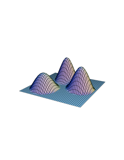
Figure 1: Logarithmic plot of the action density of a $SU(3)$ caloron (from van Baal (1999)).

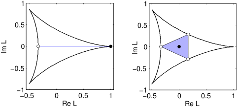
Figure 2: Schematic scatterplots (left: on the real axis, right: inside the triangle) for the local Polyakov loop values $~{}L(\vec{x})~{}$ in the complex plane, for a caloron with trivial holonomy $~{}L_{\infty}=+1~{}$ (left) and with maximally non-trivial holonomy $~{}L_{\infty}=0~{}$ (right). Black dots indicate the holonomy values, whereas white circles on the curved boundary give the Polyakov loop values at the monopole constituents according to Eq. (7) where two eigenvalues of $~{}{\mathcal{P}}~{}$ become degenerate in accordance with the monopole criterion (c) in Section I.

Provided the constituents are well separated, the Polyakov loop values at their positions $~{}\vec{y}_{m},~{}m=1,2,3~{}$ are

$${\mathcal{P}}(\vec{y}_{1}) = {\rm diag}(\hphantom{-}e^{-\pi{i}\mu_{3}},\hphantom{-}e^{-\pi{i}\mu_{3}},\hphantom{-}e^{2\pi{i}\mu_{3}}),$$

$${\mathcal{P}}(\vec{y}_{2}) = {\rm diag}(\hphantom{-}e^{2\pi{i}\mu_{1}},\hphantom{-}e^{-\pi{i}\mu_{1}},\hphantom{-}e^{-\pi{i}\mu_{1}}),$$ (7)

$${\mathcal{P}}(\vec{y}_{3}) = {\rm diag}(-e^{-\pi{i}\mu_{2}},\hphantom{-}e^{2\pi{i}\mu_{2}},-e^{-\pi{i}\mu_{2}}).$$

In Fig. 2 we illustrate the range of Polyakov loop values $~{}L(\vec{x})\equiv(1/3)~{}{\rm tr}\,{\mathcal{P}}(\vec{x})~{}$ for two limiting cases: on the left hand side for a $SU(3)$ KvB caloron with trivial holonomy $~{}L_{\infty}\equiv(1/3)~{}{\rm tr}\,{\mathcal{P}}_{\infty}=+1~{}$ which corresponds to a $SU(2)$ embedding of a Harrington-Shepard caloron Harrington and Shepard (1978) with real values of $~{}L(\vec{x})~{}$ only, and on the right hand side for maximally non-trivial holonomy $~{}L_{\infty}=0~{}$ leading to dissociated equal-mass constituents and $~{}L(\vec{x})~{}$ populating the inner triangle.

The features of KvB calorons are the following.

1. The holonomy can be chosen arbitrarily.

2. The multi-caloron contains $N~{}|Q_{\textnormal{t}}|$ constituent monopoles in accordance with various definitions.

3. The fermionic zero-mode density $\Psi_{z}^{\dagger}\Psi_{z}(x)$ is localized at the $m^{\textnormal{th}}$ constituent if $z\in(\mu_{m},\mu_{m+1})$ and jumps (delocalizes) for $z=\mu_{m}$.

These remarkable features will be illustrated for calorons of various topological charge $Q_{\textnormal{t}}$, which are obtained on asymmetric lattices, i.e. $N_{\tau}\times N_{\sigma}^{3}$ with $N_{\sigma}>N_{\tau}$, by the cooling technique. This should be seen as an illustration of an extended set of caloron solutions.

If realized on the lattice, the holonomy obviously cannot be chosen freely but dependent on the actual finite-temperature phase. Inspired by the properties listed above, Gattringer and Schaefer Gattringer (2003); Gattringer and Schaefer (2003) have analyzed a subsample of $Q_{\textnormal{t}}=\pm 1$ Monte Carlo configurations, taken from the confinement and deconfinement phase, for the localization of the (single) zero-mode with changing $~{}z~{}$. In the confinement phase, identified with maximally non-trivial holonomy, they found the pattern of zero-mode jumping. In the deconfined phase, they found a wide range in $~{}z~{}$ where the zero-mode didn’t change localization, becoming delocalized only at one angle $~{}z~{}$ corresponding to the phase of $L_{\infty}$. The localization of the zero-mode wave function was in agreement with local clusters of equal sign of the topological charge density Gattringer et al. (2004). Globally, however, the latter was far more complex than that of a single caloron.

Notwithstanding this state of affairs it is suggestive to carry over the lattice observables developed for the purpose of analyzing classical configurations to a program to rediscover superpositions of KvB calorons and anticalorons in Monte Carlo ensembles. Our aim is eventually to prove the validity of the semiclassical approach near to the transition temperature and above.

III Lattice tools of the analysis

Working on the lattice has two obvious disadvantages – the explicit breaking of scale-invariance and the existence of lattice artifacts. The classical action of a multi-caloron or instanton solution with topological charge $~{}Q_{\textnormal{t}}~{}$ is $~{}S=|Q_{\textnormal{t}}|~{}S_{\textnormal{inst}}$. It does not depend on the parameters of the solution: group orientations, positions and scale parameters. On the contrary, the standard Wilson action

$$S^{W}=\sum_{x,\mu<\nu}(1-\frac{1}{3}~{}{\rm Re}~{}{\rm tr}\,~{}U_{x,\mu\nu}),$$ (8)

depends on the scale size $~{}\rho~{}$ of an instanton discretized on the lattice. It can be calculated as Garcia Perez et al. (1994); Bruckmann et al. (2004b)

$$S^{W}_{\textnormal{inst}}=S_{\textnormal{inst}}\left(1+d_{2}\!\left(\frac{a}{\rho}\right)^{2}+\mathcal{O}(a/\rho)^{4}\right)$$ (9)

with $d_{2}=-1/5$. Hence this lattice action favors small instantons. For a KvB caloron, the intrinsic scale is determined by the constituent separations expressed by $~{}\rho_{m}~{}$, and similarly small $~{}\rho_{m}~{}$ are preferred. For $SU(2)$, in the limit of separated constituents, $~{}\rho_{m}=d~{}b/\pi^{2}~{}$ with $~{}b=1/T~{}$ and $~{}d~{}$ being the distance between the two constituents. As a remedy one could choose an (improved) action with zero or even positive coefficient $d_{2}$. For the purposes of this paper, however, we preferred to keep the numerically cheaper Wilson gauge action as the cooling action and simply to monitor the scale-size dependence.

Due to the finiteness of the lattice one cannot reproduce the $S^{1}\times\mathbb{R}^{3}$ infinite toroidal or cylindric topology. Instead, depending on the aspect ratio $N_{\tau}/N_{\sigma}$ one can interpolate between the topologies of the 4-torus $T^{4}$ and that of a cylinder. On the other hand, using the lattice as stage of such investigations has also advantages, for example the possibilities

• to produce classical fields in different topological sectors without knowing explicitly the corresponding analytic expressions,

• to include fermions into the study of solutions of the pure gauge theory,

• to test the predictions of corresponding semiclassical models and

• to explore the semiclassical structure of the respective quantized gauge field theory (also with dynamical fermions)

within one and the same framework.

In order to generate a large number of typical classical solutions of the Euclidean $SU(3)$ Yang-Mills equations of motion for a given temperature and volume, Monte Carlo lattice gauge fields have been cooled with respect to the standard Wilson gauge action. The smoothed configurations have then be characterized with the help of an $\mathcal{O}(a^{4})$ improved field strength tensor de Forcrand et al. (1997)

$$F_{\mu\nu}(x)=\frac{1}{4}\!\!\sum_{x\in\textnormal{loops}}\left[\frac{3}{2}\,W^{1,1}_{\mu\nu}-\frac{3}{20}\,W^{2,2}_{\mu\nu}+\frac{1}{90}\,W^{3,3}_{\mu\nu}\right],$$ (10)

where $~{}W^{k,l}~{}$ is the traceless and antihermitean part of the respective $k\times l$ rectangular Wilson loop. The sum is extended over the four loops of quadratic shape and each given size $~{}(n,n)~{}$ in the $\mu\nu$-plane which have the site $x$ as a common corner. From the field strength one can evaluate the corresponding improved operators of action density $s(x)$ and topological charge density $q_{\textnormal{t}}(x)$

$$s(x) = \frac{1}{2g^{2}}\;{\rm tr}\,(F_{\mu\nu}^{\,2}(x))\quad\textnormal{and}$$ (11)

$$q_{\textnormal{t}}(x) = -\frac{1}{32\pi^{2}}\,\epsilon_{\mu\nu\rho\sigma}\,{\rm tr}\,(F_{\mu\nu}(x)F_{\rho\sigma}(x)).$$ (12)

In our case of cooled gauge fields, the total topological charge $Q_{\textnormal{t}}=\sum_{x}q_{\textnormal{t}}(x)$ deviates from integer values typically by less than one percent.

The starting configurations for our cooling search have been produced by Monte Carlo simulation at $~{}\beta\equiv 6/g^{2}=5.65\,.$ For $N_{t}=4$ and $~{}6$ the Monte Carlo samples are in the confinement phase with $~{}T/T_{\textnormal{dec}}\approx 0.91$ and $0.6$, respectively. In these cases the volume average of the Polyakov loop vanishes. Under the influence of cooling this average starts to diffuse. A large fraction of configurations will approximately remain in the vicinity of maximally non-trivial holonomy until each turns into a classical solution. Various lattice sizes $~{}4\times 12^{3}$, $6\times 12^{3}$, $4\times 20^{3}$, $6\times 20^{3}$, and $12^{4}~{}$ have been chosen in order to study how the yield of classical configurations (populating different parts of the caloron parameter space) depends on the lattice size, in particular on the aspect ratio. Starting from the deconfined phase ($T>T_{\textnormal{dec}}$), mainly fields with trivial holonomy have been obtained by cooling. Throughout this paper we restrict ourselves to the confinement phase since we are mainly interested in KvB solutions with generically non-trivial holonomy.

To what extent a lattice gauge field can be regarded to be classical is measured by the violation of (anti) selfduality $\delta_{F}$, defined by

$$\delta_{F}~{}=~{}\sum_{x}~{}\left|\frac{g^{2}}{8\pi^{2}}s(x)-\left|q_{\textnormal{t}}(x)\right|\right|.$$ (13)

For a strictly selfdual or anti-selfdual gauge field this quantity vanishes.

If the caloron constituents are well-separated the action density of the caloron becomes static in $x_{0}$. An auxiliary observable which we call non-staticity

$$\delta_{t}~{}=~{}\frac{N_{t}}{4}~{}\frac{\sum_{x}{\left|s(x+\hat{0})-s(x)\right|}}{\sum_{x}s(x)}$$ (14)

has been introduced to distinguish between dissociated monopole constituents (for which the action density is static) on one hand and the non-dissociated case (which gives rise to normal time-dependent instanton lumps) on the other. The factor $N_{t}/4$ compensates for finite discretization as was chosen in previous work for $SU(2)$ Ilgenfritz et al. (2004). For classical solutions, evaluating the continuum action density Eq. (4) on a grid of points, the following benchmarks have been calculated for a symmetric set-up of the constituents. Assuming that the holonomy is maximally non-trivial, i.e. ${\rm tr}\,({\mathcal{P}_{\infty}})=0$, at least two constituents are discernible as maxima of the action density if $~{}\delta_{t}~{}$ is lower than some bifurcation value $~{}\delta_{t}^{*}=0.27$. If the non-staticity is even smaller than $~{}\delta_{t}^{**}=0.06~{}$, then it is possible to resolve all three constituents in the analytically known action density profile of the $SU(3)$ KvB caloron Martemyanov .

Unlimited cooling with the standard Wilson action will always drive the field towards a topological trivial vacuum $|Q_{\textnormal{t}}|\to 0$. In order not to loose all approximately classical fields the cooling process is monitored and a stopping condition is chosen. Using the non-staticity $\delta_{t}$ and the violation of (anti) selfduality $\delta_{F}$ we have employed two different stopping criteria which allowed us to catch an abundance of (multi-)caloron solutions in order to explore the moduli space of calorons. Cooling is stopped,

1. if the violation of (anti) selfduality $\delta_{F}$ passes through a minimum with the constraint $\delta_{F}<0.1$,

2. if either $\delta_{F}$ or the non-staticity $\delta_{t}$ passes through a minimum, depending on what happens first. Additionally the (less restrictive) constraint $\delta_{F}<0.2$ is applied.

Both criteria result in nearly (anti) selfdual gauge fields representing various topological sectors. In particular, in most cases configurations with some integer topological charge $Q_{\textnormal{t}}$ and action $S\gtrapprox S_{\textnormal{inst}}~{}|Q_{\textnormal{t}}|$ (implying a slight violation $\delta_{F}$) are found.

With the traditional choice (A) gauge fields are cooled until the equations of motion are fulfilled as good as possible and only violated to a small extent. There are some reasons to argue that this stopping condition is too strict. Superpositions of semiclassical objects (e.g. instanton and anti-instanton) are no strict solutions of the equations of motion. Nevertheless, a mixture of both must exist in a realistic model of the vacuum structure. On the other hand it is impossible to model the moduli space for an infinite $\mathbb{R}^{3}$ volume. The numerical investigation can only be done for a discrete torus, where it is known that a $|Q_{\textnormal{t}}|=1$ field can exist only at the expense of violating the (anti) selfduality Braam and van Baal (1989). Accepting a certain violation of the equation of motion constitutes a compromise between the moduli spaces of the torus and the finite temperature space-time $S^{1}\times\mathbb{R}^{3}$. Furthermore lattice artifacts of the action will bias the semiclassical content of fields. Hence one should not insist on perfect solutions of the (lattice) equations of motion. Stopping condition (B) allows to stop in an earlier stage. In particular this results in an enrichment of static, approximate classical configurations.

For a cooled gauge field configuration we determine the holonomy ${\mathcal{P}_{\infty}}$ as an average over a spatial region $V_{\alpha}$, where the action density is minimal,

$${\mathcal{P}_{\infty}} = \frac{1}{V_{\alpha}}\sum_{\vec{x}\in V_{\alpha}}\left[{\mathcal{P}}(\vec{x})\right]_{\textnormal{diagonal}}$$ (15)

$$\equiv \frac{1}{V_{\alpha}}\sum_{\vec{x}\in V_{\alpha}}{\rm diag}(e^{i\phi_{1}(\vec{x})},e^{i\phi_{2}(\vec{x})},e^{i\phi_{3}(\vec{x})})$$

with

$${\mathcal{P}}(\vec{x})=\prod_{x_{0}=1}^{N_{\tau}}U_{(x_{0},\vec{x}),0}\,.$$ (16)

The domain $V_{\alpha}$ is taken as the fraction of $\alpha=10\,\%$ of the 3-dimensional volume for which the spatial action density $\bar{s}(\vec{x})$ (the $x_{0}$-average of $s(x)$ with fixed $\vec{x}$) is smaller than everywhere in the remaining region. To get a meaningful result for the ${\mathcal{P}_{\infty}}$ operator it is necessary to choose a suitable gauge. We decided to take the Polyakov loop diagonalizing gauge, i.e. we average over the eigenvalues of ${\mathcal{P}}$. From the observed Polyakov loop operator ${\mathcal{P}}(\vec{x})$ not only the holonomy ${\mathcal{P}_{\infty}}$ (and the $\mu_{m}$’s) is determined, but also the (monopole) positions $\vec{y}_{n}$ and consequently the overall number of constituent monopoles.

Indeed, with the diagonalized Polyakov loop operator $~{}\left[{\mathcal{P}}(\vec{x})\right]_{\textnormal{diagonal}}~{}$ we identify the constituents by determining the positions $\vec{Y}$ where two eigenvalues approach each other. For the caloron solution in the continuum they would exactly coincide. On the lattice this condition has to be slightly relaxed. Thus, in our numerical work we fixed monopole positions $\vec{Y}$ through the local minima of the function

$$f(\vec{x})=\min_{i,j}|e^{i\phi_{i}(\vec{x})}-e^{i\phi_{j}(\vec{x})}|$$ (17)

in the 3-dimensional volume with the additional constraint that some $\phi$ exists such that

$$\min_{\phi\in[0,2\pi)}\left|L(\vec{Y})-(2e^{i\phi}+e^{-2i\phi})/3\,\right|<0.05.$$

This ensures that (approaching some $\phi$) the eigenvalues of ${\mathcal{P}}$ are sufficiently degenerate at $\vec{Y}$. To avoid spurious monopole positions, only monopole constituents with $~{}\bar{s}(\vec{Y})>0.1\max_{\vec{x}}\bar{s}(\vec{x})~{}$ are taken into account.

For individual configurations we also compute the spectrum of the clover-improved Wilson Dirac operator, defined as

$$\not{d}(x,y) = \delta_{x,y}-\kappa\sum_{\mu=1}^{4}\Big{[}(\mathbb{1}_{4}-\gamma_{\mu})\;U_{x,\hat{\mu}}\,\delta_{x+\mu,y}+$$

$$\hskip 56.9055pt(\mathbb{1}_{4}+\gamma_{\mu})\;U^{\dagger}_{x-\mu,\hat{\mu}}\,\delta_{x-\mu,y}\Big{]}$$

$$\not{D}(x,y) = \not{d}(x,y)+\frac{i}{2}\,\kappa\,c_{\textnormal{sw}}\,\sigma_{\mu\nu}F_{\mu\nu}(x)\,\delta_{x,y}$$

$$\qquad\text{with}\qquad\sigma_{\mu\nu}=\frac{i}{2}\left[\gamma_{\mu},\gamma_{\nu}\right].$$

The parameters are chosen to be $\kappa\!=\!1/8$ (massless) and $c_{\textnormal{sw}}\!=\!1$ (tree-level improved). For all spatial directions the boundary conditions of spinor fields are periodic, for the temporal direction one has variable ones: $\Psi_{z}(x_{0}+b,\vec{x})=e^{-2\pi iz}\;\Psi_{z}(x_{0},\vec{x})$. Eigenmodes are computed using the ARPACK package ARP .

IV Properties of lattice calorons

Under the conditions described above, different classical fields with $~{}|Q_{\textnormal{t}}|=1,\ldots,7~{}$ embedded in an arbitrary holonomy are obtained from cooling. Since the Monte Carlo simulation is performed in the confined phase, the yield of (almost) trivial holonomy configurations is low. Here we present and explain examples for $~{}|Q_{\textnormal{t}}|=0,1,2$. In order to illustrate these solutions, we provide tables with gluonic and fermionic observables.

example 1 – global observables
$S/S_{\textnormal{inst}}$	$\phantom{+}1.14$
$Q_{\textnormal{t}}$	$-1.00$
$\mu_{i}$	$\left\{\begin{array}[]{r}-0.36\\ 0.00\\ 0.36\end{array}\right\}$
$n_{+}-n_{-}$	$1-0$
$\delta_{t}$	$1.3\,\cdot 10^{-3}$
$\delta_{F}$	$0.14$

Table 1: Properties of a $Q_{\textnormal{t}}=-1$ caloron gauge field shown in Figs. 3, 4, 5 and 6.

Our first example of a $SU(3)$ classical lattice gauge field has topological charge $Q_{\textnormal{t}}=-1$ and non-trivial holonomy (cf. Tab. 1). It has been generated by cooling with respect to the standard Wilson action on a lattice of size $4\times 20^{3}$ with the stopping criterion (B). Due to the non-trivial holonomy the gauge field contains three (almost equal) massive constituent monopoles, which can be identified by the monopole criteria (a–d). These criteria coincide since the monopoles are sufficiently separated. In Fig. 3 this is made visible in the form of isosurfaces of the action density, of the function $f(\vec{x})$ according to Eq. (17) showing points, where two eigenvalues of ${\mathcal{P}}(\vec{x})$ come close to each other, as well as isosurfaces of the fermionic density for varying fermionic boundary conditions.

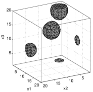
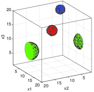
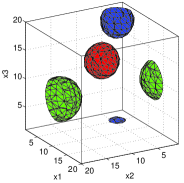
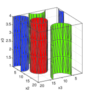
Figure 3: Caloron with non-trivial holonomy (example 1), topological charge $Q_{\textnormal{t}}=-1$ and separated constituents. We show isosurface plots for the action density (u.l.), for the function $f(\vec{x})$ (Eq. (17)) localizing the monopoles, for the fermionic density $\Psi_{z}^{\dagger}\Psi_{z}(x)$ with boundary conditions $~{}z=1/6,1/2,5/6~{}$ drawn with different colors/brightness at fixed $x_{0}$ (l.l.) and fixed $x_{1}$ (l.r.).

Evidently, the significant features of the KvB caloron of this first example are visible in Fig. 3 but the field is not perfectly anti-selfdual (compare with the $\delta_{F}$ value in Tab. 1). This effect is due to the stopping condition (B) which terminated cooling at the minimal value of $\delta_{t}$ with the constraint $\delta_{F}<0.2$.

Further cooling, until stopping condition (A) applies, would squeeze the constituents together such that no separate constituents would be visible in the action or topological charge density. Still, the Polyakov loop ${\mathcal{P}}$ and also Abelian monopoles would indicate a substructure of the single massive lump. Fermionic observables would give only a slight hint to the substructure, since the fermionic zero-mode density only slightly moves around inside the lump and is “breathing” under changes of the temporal boundary condition of the Dirac operator. It “delocalizes” to an algebraic decay at $z=\mu_{i}$. This situation is not visualized.

The clover improved Dirac operator with the background caloron field contains one zero-mode with positive chirality. The localization, measured by the inverse participation ratio $~{}\textnormal{IPR}=V~{}\sum_{x}(\Psi_{z}^{\dagger}\Psi_{z}(x))^{2}~{}$, strongly depends on the boundary condition and signals a delocalization $~{}\textnormal{IPR}\to 1~{}$ where the jumping of the zero-mode is expected to occur, namely at $~{}z=0;1/3;2/3~{}$ (cf. Fig. 4 lower right). The maximal localization is expected at $~{}z=1/6;1/2;5/6$.

Since the limit $~{}|\vec{x}|\to\infty~{}$ is not accessible on a finite lattice one might question the possibility to define the holonomy on the lattice. Nevertheless, as the upper right part of Fig. 4 shows, the eigenvalues of $~{}{\mathcal{P}}~{}$ have very small variance over the $3D$ points where the spatial action $~{}\bar{s}~{}$ is low. This property of the solution makes our definition of $~{}{\mathcal{P}_{\infty}}~{}$ a posteriori plausible. Furthermore, the eigenvalues of $~{}{\mathcal{P}}~{}$ approach each other at points with larger values of the spatial action. Since one does not observe an exact matching, the monopole criterium relying on Eq. (17) is numerically better defined. Confirming the analytic expectation, the action density is static as indicated by the small value of $~{}\delta_{t}~{}$ and resides in separated constituents.

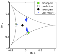
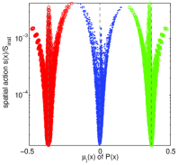
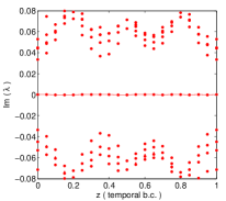
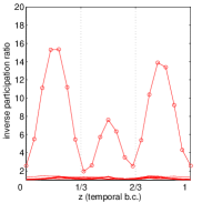
Figure 4: Caloron (example 1): scatterplot of ${\mathcal{P}}(\vec{x})$ (for the points with high enough action density) in the complex plane (u.l.); eigenvalues of ${\mathcal{P}}(\vec{x})$ versus spatial action density (eigenvalues are sorted $-0.5\leq\mu_{1}<\mu_{2}<\mu_{3}\leq 0.5$, as indicated by different points (colors/styles)) (u.r.); ${\rm Im}(\lambda)$ (eigenvalue of $\not{D}$) (l.l.) and inverse participation ratio of the lowest eigenmodes (l.r.) versus the temporal fermionic boundary condition $z$.

Fitting the lattice field by analytic expressions of the $SU(3)$ KvB caloron solution is not feasible. The numerical reconstruction of the gauge links $~{}U_{x,\mu}~{}$ in terms of the vector potential $~{}A_{\mu}(x)~{}$ is too costly. Moreover, the “latticized” analytic solutions are not yet adapted to the periodic boundary conditions. But for gauge invariant quantities like $~{}s(x)~{}$ and $~{}\Psi_{z}^{\dagger}\Psi_{z}(x)~{}$ the available analytical expressions have been easily used for a fit. The zero-mode density is (exponentially) localized only at one respective constituent for almost all angles $z$, minimizing in this way effects of the spatial boundary condition. This is shown as an example in Fig. 5 and turns out to provide a correct fit of the profile over two orders of magnitude.

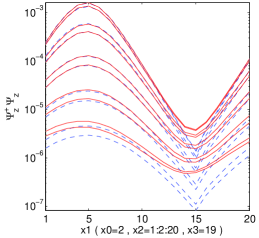
Figure 5: Fit of the analytic expression of $~{}\Psi_{z}^{\dagger}\Psi_{z}(x)~{}$ to the actual density for $~{}z=5/6~{}$; full lines means measured; dashed lines correspond the fit.

Finally let us have a look at the charge–one caloron in a maximally Abelian projection which is carried out similar to Ref. Langfeld (2004). We maximize $~{}F_{U}(D,g)={\rm Re}\;{\rm tr}\,(g(x)\,U_{x,\mu}\,g^{\dagger}(x+\hat{\mu})\,D_{x,\mu}^{\dagger})~{}$ with respect to $~{}g\in SU(3)$ and $~{}D~{}$, where $~{}D_{x,\mu}~{}$ is a $U(1)^{2}\subset SU(3)$ matrix of the form $~{}D={\rm diag}(e^{i\phi_{1}},e^{i\phi_{2}},e^{-i(\phi_{1}+\phi_{2})})~{}$. Considering the metric $~{}|U-D|^{2}={\rm tr}\,\,(U-D)^{\dagger}(U-D)~{}$ the gauge transformed link $~{}U~{}$ is required to be as close as possible to the diagonal matrix $~{}D$. Technically this is performed using the Cabibbo-Marinari method. The static electric (equal to $~{}\pm$magnetic part for an (anti)selfdual field) components of the $U(1)\times U(1)$ field strength are computed from the improved field strength tensor Eq. (10), where the $SU(3)$ links $~{}U_{x,\mu}~{}$ are replaced by the projected $~{}D_{x,\mu}$’s. The resulting field pattern is shown in Fig. 6. The maximally Abelian monopoles (sources of the electric and magnetic fields) reside inside the spheres where the Abelian field becomes singular.

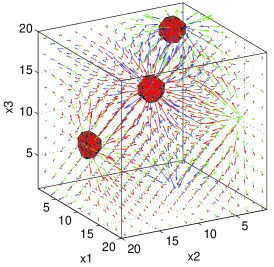
Figure 6: Abelian monopoles within a $Q_{\textnormal{t}}=-1$ caloron with non-trivial holonomy and separated constituents (example 1); colored arrows show electric ($=-$magnetic) field components of Abelian projected $U(1)\times U(1)$ field; the isosurface shows the action density of the Abelian projected field.

The second example of a selfdual lattice gauge field has $~{}Q_{\textnormal{t}}=2~{}$ and also possesses a non-trivial holonomy (cf. Tab. 2).

example 2 – global observables
$S/S_{\textnormal{inst}}$	$\phantom{+}2.04$
$Q_{\textnormal{t}}$	$\phantom{+}2.00$
$\mu_{i}$	$\left\{\begin{array}[]{r}-0.35\\ -0.01\\ 0.36\end{array}\right\}$
$n_{+}-n_{-}$	$0-2$
$\delta_{t}$	$7.4\,\cdot 10^{-3}$
$\delta_{F}$	$0.04$

Table 2: Properties of a $~{}Q_{\textnormal{t}}=2~{}$ caloron gauge field shown in Figs. 7 and 8.

It is obtained by cooling with respect to Wilson gauge action and by applying stopping condition (B). Again the expected full number of $~{}3~{}|Q_{\textnormal{t}}|=6~{}$ monopoles can be identified by the monopole criteria (b–d) – note that there are only 5 separate massive lumps visible as separate maxima in the isosurface plot of the action density and an application of criterion (a) is more subjective . The decomposition into six monopole constituents can be seen in Fig. 7.

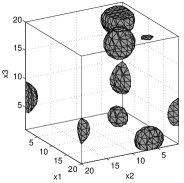
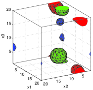
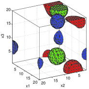
Figure 7: Caloron (example 2) with non-trivial holonomy and $~{}|Q_{\textnormal{t}}|=2$; six constituents are visible in all plots: action density (u.l.), monopoles by degenerate eigenvalues of $~{}{\mathcal{P}}(\vec{x})~{}$ (u.r.); $~{}\Psi_{z}^{\dagger}\Psi_{z}~{}$ for $~{}z=1/6,1/2,5/6~{}$ (different colors/brightness) (l.l. and l.r.).

By analyzing example 2 the results for $~{}|Q_{\textnormal{t}}|=1~{}$ are confirmed and generalized. Hence lattice calorons, especially those with non-trivial holonomy, show the typical properties of KvB calorons. Further cooling reduces the violation of the equation of motion and does not influence the constituent positions too much. However, there is a striking difference to the case $~{}|Q_{\textnormal{t}}|=1~{}$ which is a consequence of the Nahm duality Braam and van Baal (1989), which points out that classical fields with $~{}|Q_{\textnormal{t}}|=1~{}$ are unstable on the torus. In agreement with the Atiyah-Singer index theorem the $~{}Q_{\textnormal{t}}=2~{}$ field supports two zero-modes with negative chirality. The $z$-dependence of the inverse participation ratio IPR of $~{}\Psi_{z}^{\dagger}\Psi_{z}(x)~{}$ and the low lying eigenvalues of the Dirac operator are shown in the lower part of Fig. 8. The behavior of both zero-modes – the choice of basis is somewhat ambiguous – is similar to the $~{}|Q_{\textnormal{t}}|=1~{}$ case. The Polyakov loop through the constituents aligns as it is predicted by Eq. (7). The slight deviation, which can be observed in the upper left part of Fig. 8, might be due to finite volume effects. However, the upper right plot of the same figure shows that the holonomy ${\mathcal{P}_{\infty}}$ is again well defined (witnessed by the small variance of the eigenphases over the “asymptotic” subvolume $V_{\alpha}$).

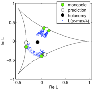
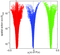
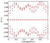
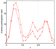
Figure 8: Caloron (example 2); scatterplot of ${\mathcal{P}}(\vec{x})$ for the points with high enough action density) in the complex plane (u.l.); eigenvalues of ${\mathcal{P}}(\vec{x})$ versus spatial action density (u.r.); ${\rm Im}(\lambda)$ (eigenvalue of $\not{D}$) (l.l.) and inverse participation ratio of the two zero-modes (l.r.) versus the temporal fermionic boundary condition $z$.

The third and last example of an almost classical gauge field has $~{}Q_{\textnormal{t}}=0~{}$ but needs to be interpreted in terms of a caloron-anticaloron superposition. The holonomy is not maximally non-trivial, giving rise

example 3 – global observables
$S/S_{\textnormal{inst}}$	$\phantom{+}2.00$
$Q_{\textnormal{t}}$	$\phantom{+}0.00$
$\mu_{i}$	$\left\{\begin{array}[]{r}-0.18\\ -0.08\\ 0.26\end{array}\right\}$
$n_{+}-n_{-}$	$0-0$
$\delta_{t}$	$6.0\,\cdot 10^{-2}$
$\delta_{F}$	$0.18$

Table 3: Properties of a caloron-anticaloron gauge field shown in Figs. 9 and 10.

to a light, a moderately large and a heavy monopole constituent (mass fractions $~{}\vec{\nu}\approx(0.1;0.35;0.55)~{}$ cf. Tab. 3). This $4\times 12^{3}$ gauge field has been cooled with respect to the standard Wilson action and again obtained under the stopping condition (B). Only $~{}4<3~{}|S/S_{\textnormal{inst}}|=6~{}$ constituents can be identified as massive lumps of action (a), which is not surprising keeping the monopole masses $8\pi^{2}\vec{\nu}$ in mind. The upper panels of Fig. 9 show the isosurfaces of action density $~{}\bar{s}(x)~{}$ and the topological charge density $~{}\bar{q}(x)$. The interpretation in terms of a caloron-anticaloron superposition is supported by the relatively large value of $~{}\delta_{F}=0.18~{}$ compared with example 2. Our choice of $~{}\delta_{F}<0.2~{}$ barely allowed us to capture this approximate solution when the non-staticity $~{}\delta_{t}~{}$ was passing a minimum. Such fields can become ultimately stable ($~{}\delta_{F}\to 0~{}$) only if the selfdual and anti-selfdual centers are infinitely separated. Any finite separation results in an attractive force between the caloron and anticaloron that renders the superposition unstable.

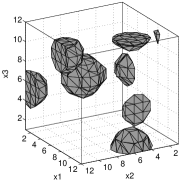
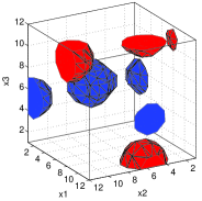
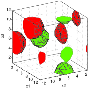
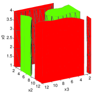
Figure 9: Caloron-anticaloron superposition (example 3) with $~{}S=2S_{\textnormal{inst}}~{}$, topological charge $~{}Q_{\textnormal{t}}=0~{}$; action density (u.l.), topological charge density (red=positive, blue=negative) (u.r.); $~{}\Psi_{z}^{\dagger}\gamma_{5}\Psi_{z}(x)~{}$ for $~{}z=0,0.5~{}$ (in different colors/brightness for each would-be zero-mode), shown in $3D$ space (l.l.) and depending on Euclidean time $x_{0}$ (l.r.).

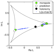
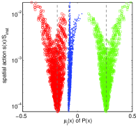
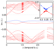
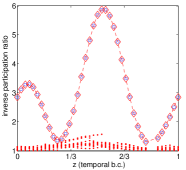
Figure 10: Caloron-anticaloron superposition (example 3): scatterplot of $~{}{\mathcal{P}}(\vec{x})~{}$ (for the points with high enough action density) in the complex plane (u.l.); eigenvalues of $~{}{\mathcal{P}}(\vec{x})~{}$ versus spatial action density (u.r.); $~{}{\rm Im}(\lambda)~{}$ (eigenvalue of $~{}\not{D}~{}$) (l.l.) and inverse participation ratio of the lowest eigenmodes (l.r.) versus the temporal fermionic boundary condition $z$.

There is no zero-mode present in this case. Instead we consider the pair of non-zero modes (with the smallest non-vanishing imaginary part of the eigenvalue $\lambda$). For this pair of modes one needs to have $~{}\langle\Psi_{z}|\gamma_{5}|\Psi_{z}\rangle=0~{}$. Hence, both eigenmodes, with $~{}{\rm Im}\lambda~{}$ positive and negative, need to be localized simultaneously on the caloron and the anticaloron for a chosen boundary condition. The characteristic jumping, presented for $~{}|Q_{\textnormal{t}}|=1,2~{}$, can be seen for the positive or negative part of $~{}\Psi_{z}^{\dagger}\gamma_{5}\Psi_{z}(x)~{}$. Both parts enclose lumps of action with the same sign of topological density. The flow of the inverse participation ratio IPR of the eigenmode density in Fig. 10 still shows two similarly localized eigenmodes (cf. circles and diamonds in the lower right panel). In the same plot it is visible that the modes only delocalize twice, which would support an interpretation in terms of an embedded $SU(2)$ caloron–anticaloron. This is actually not the case, e.g. the scatterplot of the Polyakov loop clearly exhibits a scattering in the full complex plane, which is not possible for a trivial $SU(2)$ embedding. The interpretation in terms of a KvB caloron is still valid, however, the behavior of a superposition of fields with opposite duality differs from a fully selfdual or anti-selfdual caloron.

V Ensembles of lattice calorons

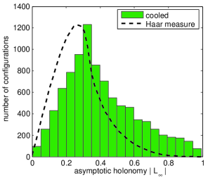
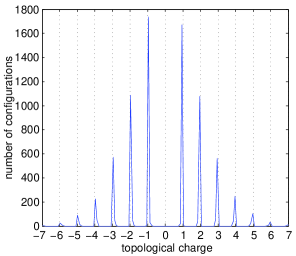
Figure 11: Histogram of $|{\rm tr}\,{\mathcal{P}_{\infty}}|/3$ (left) and $Q_{\textnormal{t}}$ (right) for $4\times 12^{3}$ (stopping condition (B)).

To underline the importance of classical solutions with non-trivial holonomy we show on the left in Fig. 11 a distribution of the modulus of the average of $~{}L(\vec{x})~{}$, which would be equal to one for trivial holonomy ${\mathcal{P}_{\infty}}\in Z(3)$ and smaller for non-trivial holonomy. It shows primarily that we are investigating properties of classical fields with a non-trivial holonomy and that these fields can be produced by cooling on the lattice. The distribution of topological charges on the right in Fig. 11 shows the available range of topological sectors. The case $~{}Q_{\textnormal{t}}=0~{}$ is excluded, because configurations of this class mostly pass cooling without being stopped before they reach very low action (the third example above is a fortunate exception just tolerated by $~{}\delta_{F}<0.2$). Both distributions only weakly depend on the stopping condition. The distributions of the non-staticity $\delta_{t}$ and of the violation of selfduality (i.e. of the equation of motion) $\delta_{F}$ naturally depend on the stopping condition. According to condition (A) cooling proceeds until the equation of motion is maximally fulfilled. In this (actually late) stage the constituents are already squeezed. In the corresponding ensemble of cooled configurations one cannot find static calorons with separated constituents, at least for $~{}|Q_{\textnormal{t}}|=1~{}$ where squeezing is found to be a particularly strong effect. With the help of the non-staticity this role of the stopping criteria is visualized in the upper panels of Fig. 12 – with stopping condition (A) (upper right plot) no static calorons with $~{}|Q_{\textnormal{t}}|=1~{}$ ($\delta_{t}/\delta_{t}^{*}\ll 1$ ) are found, whereas the combined stopping condition (B) (upper left plot) gives both static (peak (a)) and non-static calorons (peak (b)) with $~{}|Q_{\textnormal{t}}|=1$. This effect is much weaker for $~{}|Q_{\textnormal{t}}|=2,\ldots,4$.

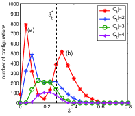
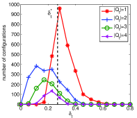
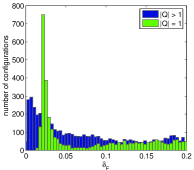
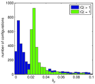
Figure 12: Distribution of non-staticity $\delta_{t}$ (upper) and of the violation of (anti) selfduality $\delta_{F}$ (lower) for stopping condition (A) (right) and (B) (left).

For the general understanding it is also interesting to know how the violation of selfduality $\delta_{F}$ is distributed. For both stopping criteria this is shown in the lower panels of Fig. 12. Clearly, the case $~{}|Q_{\textnormal{t}}|=1~{}$ appears exceptional also in this respect since it has a positive lower bound for the violation of (anti)selfduality of $~{}\approx 0.02~{}$ in contrast to classical configurations with $~{}|Q_{\textnormal{t}}|>1$.

The previous figures describe the composition of the ensembles. In order to characterize better the composition of the configurations one should choose observables closer related to the KvB caloron solution. It would be most natural to count the constituent monopoles inside the caloron configurations. For this purpose we apply the definition of a monopole as sitting at $\vec{Y}$ by two coinciding eigenvalues of ${\mathcal{P}}(\vec{Y})$, which was explained in Chapter III. Additionally we show in Fig. 13 the number of dominant (i.e. $~{}|q_{\textnormal{t}}(Y)|>0.1\max_{x}|q_{\textnormal{t}}(x)|~{}$) local extrema in the topological charge density for the ensemble produced with stopping condition (B).

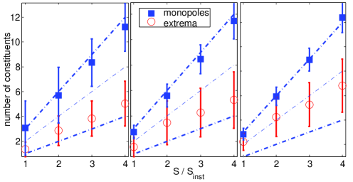
Figure 13: Number of constituents for $4\times 12^{3}$ ensemble with standard deviation (bars); full squares by “coinciding of eigenvalues” criterion, open circles from local maxima in the 4D action density; (left) full ensemble; (middle) with $L_{\infty}<0.2$ and (right) with $\delta_{t}<0.1$ and $L_{\infty}<0.2$.

Both methods, the number of monopoles provisionally defined as local maxima of the action/topological charge density or by our actually adopted monopole definition, expose (cf. in Fig. 13) always more than $|Q_{\textnormal{t}}|$ lumps, a situation that would be expected for a caloron with massless or close-by constituents. With the actual monopole definition, on average $3|Q_{\textnormal{t}}|$ monopoles are found in each topological sector. This is independent of the cut, which can be applied to the ensemble to make the monopole counting better defined. By applying more strict cuts to the ensemble (with respect to the holonomy and non-staticity, from left to right in Fig. 13) the standard deviation of the number of monopoles for given $~{}S/S_{\textnormal{inst}}~{}$ decreases while on average the expectation to find $~{}3~{}|Q_{\textnormal{t}}|~{}$ monopoles is reconfirmed.

The splitting into static and non-static configurations in the distribution of the non-staticity (cf. upper left in Fig. 12) for stopping condition (B) is also reproduced looking at the distribution of the average monopole distance in Fig. 14. In this Fig. the sample is restricted to configurations with $|Q_{t}|=1$ where 3 monopoles have been observed. The correspondence between the clustering into static and non-static sets of configurations in Fig. 12 and Fig. 14 is highlighted by labelling those clusters of events (in both figures) as (a) and (b). They have emerged from the cooling process either because of the non-staticity went through a minimum (cluster (a)) or the violation of the equation of motion was minimal (cluster (b)).

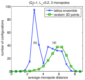
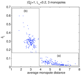
Figure 14: Distribution of the average pairwise monopole distances compared with the result of an uniform distribution of 3D points (left). Average monopole distance versus the non-staticity $\delta_{t}$.

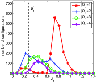
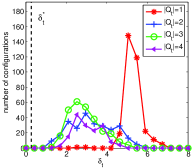
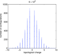
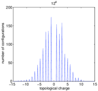
Figure 15: Distribution of non-staticity (upper) and topological charges (lower) for the $6\times 12^{3}$ (left) and $12^{4}$ (right) ensembles.

In Fig. 14 it becomes clear by comparison that the first cluster (a) is well represented by calorons with constituents uniformly distributed on the lattice. The average distance is comparably large and consequently they are static. On the other hand, configurations forming cluster (b) have emerged from cooling because of a minimal violation of the equation of motion achieved in a later stage of cooling. The constituents are squeezed and the action density has become non-static, which can be monitored during cooling by increasing values of $\delta_{t}$.

The correlation between non-staticity and monopole distance qualitatively satisfies the analytical expectation while the effect of the stopping condition reflects the expected, unavoidable side-effect of cooling with respect to the standard Wilson action.

To understand what changes when the temperature is lowered at fixed volume and approaches zero temperature (on the symmetric torus) we have studied the same properties for an ensemble on a $6\times 12^{3}$ and a $12^{4}$ lattice. $N_{\tau}$ and $N_{\sigma}$ together (by the aspect ratio of the lattice) characterize to what extent finite $T$ in infinite volume, $S^{1}\times\mathbb{R}^{3}$, is modeled. Only if $~{}N_{\sigma}\gg N_{\tau}~{}$ the caloron finite volume effects (caused by overlapping constituents) can be neglected. By sending $~{}N_{\tau}\to N_{\sigma}~{}$ and keeping the size (and distance) of the object small compared to the box length, more instanton-like classical solution are expected.

In our earlier $SU(2)$ lattice studies a recombination of dissociated caloron constituents into a single non-dissociated object, still with non-trivial holonomy, has been observed in the limit $~{}N_{\tau}\to N_{\sigma}~{}$ Ilgenfritz et al. (2004) . We repeat this study for $SU(3)$ by using lattices with aspect ratios $~{}N_{\tau}/N_{\sigma}=6/12~{}$ and $~{}N_{\tau}/N_{\sigma}=12/12~{}$ in creating ensembles of configurations cooled until the stopping condition (B) is satisfied. In complete analogy to the $SU(2)$ case static calorons disappear if the aspect ratio $~{}N_{\tau}/N_{\sigma}~{}$ is increased (upper part of Fig. 15). In Fig. 16 the number of constituents, found for different topological sectors $~{}|Q_{\textnormal{t}}|~{}$, for $N_{\tau}=6$ is shown. Different cuts with respect to the holonomy $|{\mathcal{P}_{\infty}}|$ and non-staticity $\delta_{t}$ are applied.

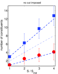
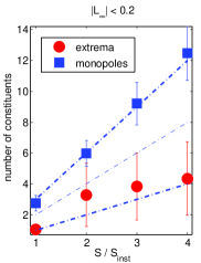
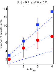
Figure 16: Dissociation into constituents from local maxima of action and monopole counting (defined by coinciding eigenvalues) for $6\times 12^{3}$ lattice with different cuts imposed.

Despite the bigger aspect ratio $3~{}|Q_{\textnormal{t}}|$ monopoles are still visible whereas a smaller number of local extrema is observed in the topological charge density, closer to one lump per unit charge, if no further cuts with respect to holonomy and non-staticity are applied. Since the interpretation of the Polyakov loop (corresponding to a choice of a “time” direction) would be ambiguous, this has not been checked on the symmetric lattice. We would like to remind the reader that Gattringer and Pullirsch Gattringer and Pullirsch (2004) have found on the symmetric torus, similar to the observations at $T\neq 0$  Gattringer and Schaefer (2003), jumping of the zero-mode for $Q_{\textnormal{t}}=\pm 1$ Monte-Carlo configurations under a change of boundary conditions. In the light of the present studies we would doubt an interpretation in terms of jumping between fractionally-charged constituents.

VI Conclusions

We have applied cooling to $SU(3)$ Monte Carlo fields in the confined phase at finite temperature. The typical KvB behavior of these fields was shown for examples with $~{}|Q_{\textnormal{t}}|=1,2~{}$ and $~{}Q_{\textnormal{t}}=0~{}$ by analyzing field strength, Polyakov loop, action and topological charge profiles and the behavior of low-lying modes of the Dirac operator. This part was complemented by studying the content of the whole ensemble, especially with respect to the monopole content of solutions in each topological charge sector. The outcome is biased by the choice of lattice action – we have used the standard Wilson action – which can be compensated by a suitable stopping condition for the cooling iteration. Still, $~{}|Q_{\textnormal{t}}|=1~{}$ plays an exceptional role. However, in agreement with the analytical expectation we find $~{}3~{}|Q_{\textnormal{t}}|~{}$ constituent monopoles (for $~{}|Q_{\textnormal{t}}|=1,\dots,4~{}$) which are defined by the coincidence of two eigenvalues of $~{}{\mathcal{P}}(\vec{x})~{}$.

Zero modes of the Dirac operator with adjustable boundary conditions are an useful filter to explore the semiclassical structure. Chirally improved Dirac operators are necessary for the study of its low-lying modes to be applicable directly to unsmeared Monte Carlo configurations. Using the full feature of exploring the spectral flow depending on the boundary condition leads to high computational costs such that only small samples of configurations can be studied.

Uncovering the topological structure requires one to introduce notion of smoothness. Therefore smearing has been applied to explore the topological density or the action density. Both observables can give valuable information about the lattice configuration already after some amount of cooling or smearing. Nevertheless, one might miss significant features of KvB calorons by relying only on those. Having the connection between the holonomy and deconfinement-confinement phase transition in mind, the Polyakov loop operator is another very important and valuable tool to investigate the classical properties. The signature of a monopole is that $~{}L(\vec{x})\equiv(1/3)~{}{\rm tr}\,{\mathcal{P}}(\vec{x})~{}$ is close to the envelope of the range of the Polyakov loop (see the upper left panel of Fig. 4). But it is unlikely that this signature can be directly observed in an early stage of smearing or cooling.

In future investigations we will use these tools to explore the properties of finite temperature lattice field theory near the $SU(3)$ deconfinement–confinement phase transition by applying different smearing techniques. Lattice studies can hopefully help to identify the dissociation of calorons with non-trivial holonomy if the temperature is lowered below the critical one, in other words, to verify the semiclassical results.

VII Acknowledgements

We thank P. van Baal, F. Bruckmann, Ch. Gattringer, B. Martemyanov, A. Schäfer, St. Solbrig and A. Veselov for numerous exciting discussions, in particular P. van Baal, F. Bruckmann and Ch. Gattringer for a careful reading of the manuscript. E.-M. I. and M. M.-P. acknowledge financial support by the DFG (FOR 465 / Mu 932/2). D. P. has been supported by the DFG Graduate School GRK 271.

Appendix A Auxiliary fields

The auxiliary fields for the construction of $SU(3)$ $~{}|Q_{\textnormal{t}}|=1~{}$ calorons are Kraan and van Baal (1998c):

$$\psi(x_{0},\vec{x}) = \frac{1}{2}\,{\rm tr}\,(\mathcal{A}_{3}\,\mathcal{A}_{2}\,\mathcal{A}_{1})-\cos(2\pi x_{0}),$$

$$\mathcal{A}_{m}(\vec{x}) = \frac{1}{r_{m}}\begin{pmatrix}r_{m}&|\vec{\rho}_{m+1}|\\ 0&r_{m+1}\end{pmatrix}\begin{pmatrix}{\rm ch_{m}}&{\rm sh_{m}}\\ {\rm sh_{m}}&{\rm ch_{m}}\end{pmatrix}$$

using the notation ${\rm ch_{m}}=\cosh(2\pi\nu_{m}r_{m})$, ${\rm sh_{m}}=\sinh(2\pi\nu_{m}r_{m})$, $r_{m}=|\vec{x}-\vec{y}_{m}|$ and $\vec{\rho}_{m}=\vec{y}_{m}-\vec{y}_{m-1}$.

The fermionic density is derivable from the Green’s function $\hat{f}_{x}$

$$\hat{f}_{x}(z,z^{\prime}) = \frac{\pi e^{2\pi it(z-z^{\prime})}}{r_{m}\psi}\Big{[}e^{-2\pi it}\sinh(2\pi r_{m}(z-z^{\prime}))$$

$$+ \langle v_{m}(z^{\prime})|\pi(\mathcal{A}_{3}\mathcal{A}_{2}\mathcal{A}_{1})|w_{m}(z)\rangle\Big{]},$$

with

$$v_{m}^{1}(z) = -w_{m}^{2}(z)=\sinh(2\pi r_{m}(z-\mu_{m})),$$

$$v_{m}^{2}(z) = \phantom{-}w_{m}^{1}(z)=\cosh(2\pi r_{m}(z-\mu_{m})).$$

The construction of the caloron field $A_{\mu}$ requires the knowledge of the following matrix fields $C_{\alpha}$ and $\phi$:

$$(C_{\alpha})_{mk} = \zeta_{m}\bar{\eta}_{\alpha\beta}\;\zeta_{k}^{\dagger}\,\partial_{\beta}\hat{f}_{x}(\mu_{m},\mu_{k}),$$

$$\left(\phi^{-1}\right)_{mk} = \delta_{mk}-\zeta_{m}\zeta_{k}^{\dagger}\;\hat{f}_{x}(\mu_{m},\mu_{k}).$$

The anti-selfdual ’t Hooft symbols are $~{}\bar{\eta}_{\alpha\beta}=\bar{\sigma}_{[\alpha}\sigma_{\beta]}$. The permutation $~{}\pi(\mathcal{A}_{3}\mathcal{A}_{2}\mathcal{A}_{1})~{}$ is $~{}\mathcal{A}_{3}\mathcal{A}_{2}\mathcal{A}_{1}$, $~{}\mathcal{A}_{1}\mathcal{A}_{3}\mathcal{A}_{2}~{}$ or $~{}\mathcal{A}_{2}\mathcal{A}_{1}\mathcal{A}_{3}~{}$ for $~{}m=1,2$ or $3$, respectively. In the expression for $~{}\hat{f}~{}$ the assumption $~{}\mu_{m}\!\leq\!z^{\prime}\!\leq\!z\!\leq\!\mu_{m+1}~{}$ has been made. This can be generalized by $~{}\hat{f}_{x}(z^{\prime},z)\!=\!\hat{f}_{x}^{*}(z,z^{\prime})$. If the constituent positions $~{}\vec{y}_{m}~{}$ lie in the $~{}x_{1}-x_{2}~{}$ plane, one can use $~{}\zeta_{m}=(|\vec{\rho}_{m}|,i\rho_{m}^{2}-\rho_{m}^{1})/\sqrt{2\pi|\vec{\rho}_{m}|}$. In general one has $~{}\vec{\rho}_{m}=-\pi\zeta_{m}\vec{\tau}\zeta_{m}^{\dagger}~{}$ with the Pauli vector $~{}\vec{\tau}=(\tau_{1},\tau_{2},\tau_{3})$. The temporal shift $~{}y_{0}~{}$ is set to zero and $~{}b\;=\;1/T\;=\;1~{}$ throughout these formulas. The angles $~{}\mu_{m}~{}$ are determined by the holonomy $~{}{\mathcal{P}_{\infty}}\simeq\exp(2\pi i\;{\rm diag}(\mu_{1},\mu_{2},\mu_{3}))$.

References

- ’t Hooft (1976) G. ’t Hooft, Phys. Rev. D14, 3432 (1976).
- Callan et al. (1978) J. Callan, Curtis G., R. F. Dashen, and D. J. Gross, Phys. Rev. D17, 2717 (1978).
- Coleman (1977) S. R. Coleman (1977), lecture delivered at 1977 Int. School of Subnuclear Physics, Erice, Italy, Jul 23-Aug 10, 1977.
- Belavin et al. (1975) A. A. Belavin, A. M. Polyakov, A. S. Shvarts, and Y. S. Tyupkin, Phys. Lett. B59, 85 (1975).
- Atiyah et al. (1978) M. F. Atiyah, N. J. Hitchin, V. G. Drinfeld, and Y. I. Manin, Phys. Lett. A65, 185 (1978).
- Ilgenfritz and Müller-Preussker (1981) E.-M. Ilgenfritz and M. Müller-Preussker, Nucl. Phys. B184, 443 (1981).
- Shuryak (1982) E. V. Shuryak, Nucl. Phys. B203, 93 (1982).
- Diakonov and Petrov (1984) D. Diakonov and V. Y. Petrov, Nucl. Phys. B245, 259 (1984).
- Schäfer and Shuryak (1998) T. Schäfer and E. V. Shuryak, Rev. Mod. Phys. 70, 323 (1998), eprint hep-ph/9610451.
- Diakonov (2003) D. Diakonov, Prog. Part. Nucl. Phys. 51, 173 (2003), eprint hep-ph/0212026.
- Negele et al. (2004) J. W. Negele, F. Lenz, and M. Thies (2004), eprint hep-lat/0409083.
- Gross et al. (1981) D. J. Gross, R. D. Pisarski, and L. G. Yaffe, Rev. Mod. Phys. 53, 43 (1981).
- Harrington and Shepard (1978) B. J. Harrington and H. K. Shepard, Phys. Rev. D17, 2122 (1978).
- Kraan and van Baal (1998a) T. C. Kraan and P. van Baal, Nucl. Phys. B533, 627 (1998a), eprint hep-th/9805168.
- Lee and Lu (1998) K.-M. Lee and C.-H. Lu, Phys. Rev. D58, 025011 (1998), eprint hep-th/9802108.
- Prasad and Sommerfield (1975) M. K. Prasad and C. M. Sommerfield, Phys. Rev. Lett. 35, 760 (1975).
- Bogomol’nyi (1976) E. B. Bogomol’nyi, Sov. J. Nucl. Phys. 24, 449 (1976).
- van Baal (2002) P. van Baal, Nucl. Phys. Proc. Suppl. 106, 586 (2002), eprint hep-lat/0108027.
- Diakonov et al. (2004) D. Diakonov, N. Gromov, V. Petrov, and S. Slizovskiy, Phys. Rev. D70, 036003 (2004), eprint hep-th/0404042.
- Diakonov (2004) D. Diakonov (2004), eprint hep-ph/0407353.
- Kraan (2000) T. C. Kraan, Commun. Math. Phys. 212, 503 (2000), eprint hep-th/9811179.
- Diakonov and Gromov (2005) D. Diakonov and N. Gromov (2005), eprint hep-th/0502132.
- Ilgenfritz et al. (2002) E.-M. Ilgenfritz, B. V. Martemyanov, M. Müller-Preussker, S. Shcheredin, and A. I. Veselov, Phys. Rev. D66, 074503 (2002), eprint hep-lat/0206004.
- Ilgenfritz et al. (2004) E.-M. Ilgenfritz, B. V. Martemyanov, M. Müller-Preussker, and A. I. Veselov, Phys. Rev. D69, 114505 (2004), eprint hep-lat/0402010.
- Ilgenfritz et al. (2005) E.-M. Ilgenfritz, B. V. Martemyanov, M. Müller-Preussker, and A. I. Veselov, Phys. Rev. D71, 034505 (2005), eprint hep-lat/0412028.
- Bruckmann and van Baal (2002) F. Bruckmann and P. van Baal, Nucl. Phys. B645, 105 (2002), eprint hep-th/0209010.
- Braam and van Baal (1989) P. J. Braam and P. van Baal, Commun. Math. Phys. 122, 267 (1989).
- Nye (2001) T. M. W. Nye (2001), eprint hep-th/0311215.
- Ward (2004) R. S. Ward, Phys. Lett. B582, 203 (2004), eprint hep-th/0312180.
- Bruckmann et al. (2004a) F. Bruckmann, D. Nogradi, and P. van Baal, Nucl. Phys. B698, 233 (2004a), eprint hep-th/0404210.
- Kraan and van Baal (1998b) T. C. Kraan and P. van Baal, Nucl. Phys. A642, 299 (1998b), eprint hep-th/9805201.
- Kraan and van Baal (1998c) T. C. Kraan and P. van Baal, Phys. Lett. B435, 389 (1998c), eprint hep-th/9806034.
- van Baal (1999) P. van Baal (1999), eprint hep-th/9912035.
- Gattringer (2003) C. Gattringer, Phys. Rev. D67, 034507 (2003), eprint hep-lat/0210001.
- Gattringer and Schaefer (2003) C. Gattringer and S. Schaefer, Nucl. Phys. B654, 30 (2003), eprint hep-lat/0212029.
- Gattringer et al. (2004) C. Gattringer, E.-M. Ilgenfritz, B. V. Martemyanov, M. Müller-Preussker, D. Peschka, R. Pullirsch, S. Schaefer, and A. Schäfer, Nucl. Phys. Proc. Suppl. 129, 653 (2004), eprint hep-lat/0309106.
- Garcia Perez et al. (1994) M. Garcia Perez, A. Gonzalez-Arroyo, J. Snippe, and P. van Baal, Nucl. Phys. B413, 535 (1994), eprint hep-lat/9309009.
- Bruckmann et al. (2004b) F. Bruckmann, E.-M. Ilgenfritz, B. V. Martemyanov, and P. van Baal, Phys. Rev. D70, 105013 (2004b), eprint hep-lat/0408004.
- de Forcrand et al. (1997) P. de Forcrand, M. Garcia Perez, and I.-O. Stamatescu, Nucl. Phys. B499, 409 (1997), eprint hep-lat/9701012.
- (40) B. Martemyanov, private communication.
- (41) Arpack code package, see www.caam.rice.edu/software/ARPACK.
- Langfeld (2004) K. Langfeld, Phys. Rev. D69, 014503 (2004), eprint hep-lat/0307030.
- Gattringer and Pullirsch (2004) C. Gattringer and R. Pullirsch, Phys. Rev. D69, 094510 (2004), eprint hep-lat/0402008.