A gauge-invariant object in non-Abelian gauge theory

Abstract

We propose a nonlocal definition of a gauge-invariant object in terms of the Wilson loop operator in a non–Abelian gauge theory. The trajectory is a closed curve defined by an (untraced) Wilson loop which takes its value in the center of the color group. We show that definition shares basic features with the gauge-dependent ’t Hooft construction of Abelian monopoles in Yang-Mills theories. The chromoelectric components of the gluon field have a hedgehog-like behavior in the vicinity of the object. This feature is dual to the structure of the ’t Hooft-Polyakov monopoles which possesses a hedgehog in the magnetic sector. A relation to color confinement and lattice implementation of the proposed construction are discussed.

I Introduction

The mechanism of color confinement in QCD is an important problem which is not yet solved. An approach by Nambu, ’t Hooft and Mandelstam ref:DualSuperconductor suggests that the vacuum of QCD can be treated as a dual superconductor, which confines quarks due to presence of special configurations of gluon fields called “Abelian monopoles”. In brief, if the monopoles are condensed then the chromoelectric flux of (anti-) quarks is squeezed into tubes (“QCD strings”) which confine quarks and anti-quarks into tightly bound colorless bound states. Features of this mechanism and results of corresponding numerical studies on the lattice – which confirm the validity of the dual superconductor mechanism in a particular gauge of the Yang-Mills theory – can be found in reviews ref:Reviews .

The basic element of the dual superconductor approach is the Abelian monopole. The existence of this object is not supported by the symmetries of QCD. However, the monopoles can be identified with particular configurations of the gluon fields by the so-called Abelian projection formalism invented by ’t Hooft ref:thooft:monopole . This formalism relies on a partial gauge fixing of the $SU(N)$ gauge symmetry up to an Abelian subgroup. The Abelian monopoles appear naturally in the Abelian gauge as a result of the compactness of the residual Abelian group.

One of the major problems associated with the ’t Hooft construction of the monopole in pure gauge theories is that this construction is not universal. Or, as often said, the construction is gauge dependent: the location of the monopole in a fixed gluon field configuration is dependent of the gauge fixing matrix $X$ (to be defined in the next Section). There is an infinite number of such matrices, and, respectively, there is an infinite number of the Abelian monopole definitions in non-Abelian gauge theories. Some (if not most) of the definitions are physically irrelevant for infrared problems such as the confinement problem. For example, the Abelian monopoles existing in the Polyakov Abelian gauge – which is defined by diagonalization of the Polyakov loop – are always static in the continuum limit ref:Yukawa ; ref:Polyakov:gauge , and they cannot contribute to the confinement of the static quarks. On the other hand, the monopoles defined in the so-called Maximal Abelian gauge ref:MA were numerically shown to make a dominant contribution to the confinement of quarks ref:monopole:dominance as well as to other low-energy non-perturbative phenomena.

Clearly, the gauge invariant phenomena (such as the quark confinement) can not be described by the gauge-dependent mechanism. Probably, one should blame the tool of Abelian projections which is used to ”detect” the monopoles: the monopoles (as confining defects) are observed well in one gauge and they are “eaten up” or contaminated by artifacts in another gauge.

There were various attempts to find an appropriate solution of the gauge-dependence problem of the monopole-based confinement mechanism. Some approaches ref:continuum ; ref:Fedor ; ref:Faber are based on an attempt to find a gauge invariant definition of Abelian monopoles in non-Abelian gauge theories. Another approach ref:Suzuki:Landau pays attention to the magnetic displacement currents observed in the Landau gauge. The displacement is linked to the existence $A^{2}$ condensate ref:A2 which should contain a gauge–invariant piece. On the other hand the authors of Ref. ref:Alex claim that in a pure non-Abelian gauge theory the monopole charge can not be defined at all. This claim is opposed by Ref. ref:reply:Alex .

In this paper we propose a construction of a new gauge-invariant object in non-Abelian gauge theories, which may have a tight link to the confinement phenomena. The basic idea is to use the Wilson loop variable as an effective path-dependent Higgs field which allows to define a singularity in self-consistent way. The construction resembles the ’t Hooft definition of the Abelian monopole but does not rely on any gauge fixing procedure.

The structure of the paper is as follows. In Section II we briefly overview the Abelian monopoles defined in the Abelian projection formalism. In Section III we show how the gauge-invariant object can uniquely be constructed in a manner similar to the Abelian monopoles. A relation to the confinement of color and a possible lattice implementation of the proposed construction are also discussed. In Section IV we consider examples of specific gluon field configurations and show that our definition correctly recognizes a self-dual BPS monopole. We also discuss dynamics of our objects at a finite-temperature as well as in lower dimensions. The last Section contains our conclusion.

II ’t Hooft’s Abelian monopoles in SU(N) gauge theories

The ’t Hooft definition of an Abelian monopole ref:thooft:monopole in non–Abelian gauge theories is based on a partial gauge fixing of the non–Abelian gauge freedom up to the Abelian one. Technically, the Abelian gauge fixing is achieved by diagonalization of an arbitrary adjoint operator $X(x)\equiv X^{a}T^{a}$, where $T^{a}$ are the generators of the $SU(2)$ group, $a=1,\dots,N^{2}-1$. In the Abelian gauge the operator $X$ is diagonalized by the gauge transformations in the whole space-time:

$$X(x)\to X^{\prime}(x)\equiv\Omega^{\dagger}(x)\,X(x)\,\Omega(x)={\mathrm{diag}}\Bigl{(}\lambda_{1}(x),\lambda_{2}(x),\dots,\lambda_{N}(x)\Bigr{)}\equiv X_{\mathrm{diag}}(x)\,,$$ (1)

where $\Omega$ is the matrix of the $SU(N)$ gauge transformation and $\lambda_{1}\geqslant\lambda_{2}\geqslant\dots\geqslant\lambda_{N}$.

From Eq. (1) one sees that the gauge can not be fixed completely since the diagonal operator $X_{\mathrm{diag}}$ remains intact under arbitrary Abelian ${[U(1)]}^{N-1}$ gauge transformations given by matrices

$$\Omega^{\mathrm{Abel}}={\mathrm{diag}}\Bigl{(}e^{i\alpha_{1}(x)},e^{i\alpha_{2}(x)},\dots,e^{i\alpha_{N}(x)}\Bigr{)}\,,\qquad\sum^{N}_{a=1}\alpha_{a}(x)=1\,,$$ (2)

where $\alpha_{i}(x)\in[0,2\pi)$ are arbitrary functions which obey the $SU(N)$–imposed constraint.

After the $SU(N)\to{[U(1)]}^{N-1}$ gauge fixing (1) the model not only respects the Abelian gauge invariance but it also possesses the topological defects called Abelian monopoles ref:thooft:monopole . The Abelian monopoles come from singularities of the gauge fixing condition (1). If at the point $x_{0}$ two eigenvalues of the diagonalized $X$-matrix coincide (say, $\lambda_{i}(x_{0})=\lambda_{i+1}(x_{0})$) then at this point the Abelian gauge can not be fixed by the condition (1). In other words, in the point $x_{0}$ the matrix of the residual gauge transformations is no more diagonal contrary to the Abelian matrix (2). Formally, the residual gauge transformations also contain the $SU(2)$ subgroup embedded into the $SU(N)$ group at the place where the columns with the numbers $i$ and $i+1$ overlap with the rows $i$ and $i+1$.

Below we consider the $SU(2)$ group. The generalization to the $SU(N)$ case is simply given by repeating of the $SU(2)$ considerations with respect to the $i$ and $i+1$ columns/rows of the $SU(N)$ $X$-matrix with coinciding eigenvalues $\lambda_{i}(x_{0})=\lambda_{i+1}(x_{0})$. In the $SU(2)$ case, $X=X^{a}\sigma^{a}/2$ where $\sigma^{a}$, $a=1,2,3$ are the Pauli matrices, and the diagonal matrix is $X_{\mathrm{diag}}={\mathrm{diag}}\bigl{(}\lambda,-\lambda\bigr{)}$ with $\lambda>0$. The gauge fixing singularities appear at points of the space-time where the $X$-matrix is degenerate,

$$X(x)=0\,,$$ (3)

i.e. where $\lambda(x)=0$. Since $\lambda(x)=(1/2){\bigr{(}\sum^{3}_{a=1}X^{a,2}\bigl{)}}^{1/2}$, the single condition $\lambda(x)=0$ is equivalent to the three independent constraints $X^{a}(x)=0$, $a=1,2,3$. These three constraints in four-dimensional space-time define a loop (or, a set of loops). This loop is the world trajectory of the Abelian monopole. One can show that the monopole charge is conserved ref:thooft:monopole ; ref:general:singularities .

Consider the point $x_{0}$ at the monopole trajectory. Without loosing of generality let us assume that the monopole current is pointing out towards 4th direction. Then the matrix $X$ has the following spatial structure in the vicinity of the monopole:

$$X(x)=\frac{\sigma^{a}}{2}\,Y^{ai}{\bigl{(}x-x_{0}\bigr{)}}^{i}+O\Bigl{(}\bigl{(}x-x_{0}\bigr{)}^{2}\Bigr{)}\,,\qquad Y^{ai}\equiv\frac{\partial X^{a}(x)}{\partial x^{i}}{\Biggl{|}}_{x=x_{0}}\,,\qquad a,i=1,2,3.$$ (4)

If the $Y$–matrix is not degenerate, ${\mathrm{det}}Y\neq 0$, then the point $x_{0}$ corresponds to the isolated singularity point (which is the general case to be considered below).

Using the change of variables in Eq. (4), $x_{i}\to y_{i}={(Y^{-1})}_{ia}(x-x_{0})^{a}$, we transform the $X$-matrix to the canonical form: $X=(\sigma^{a}/2)\,y_{a}+O(y^{2})$. Thus, in the vicinity of the singularity, the field $X$ has a hedgehog form resembling the behavior of the adjoint Higgs field in the vicinity of the ’t Hooft-Polyakov monopole solution ref:tHooft:GGmonopole ; ref:Polyakov:GGmonopole of the Georgi–Glashow model. In order to figure out that the singularity in the Abelian gauge corresponds indeed to an Abelian monopole, one notes that a gauge transformation – which diagonalizes the singular hedgehog configuration into the regular (diagonal) configuration – must itself be singular. Using the standard parameterization, ${\mathbf{y}}=r\,(\sin\theta,\cos\varphi,\sin\theta,\sin\varphi,\cos\theta)$, one can write the matrix $X$ and the diagonalization matrix $\Omega$, Eq. (1), as follows (we omit $O(y^{2})$ corrections below):

$$X=\frac{r}{2}\left(\begin{array}[]{lr}\cos\theta&e^{-i\varphi}\sin\theta\\ e^{i\varphi}\sin\theta&-\cos\theta\\ \end{array}\right)\,,\qquad\Omega=\left(\begin{array}[]{lr}\cos{\theta/2}&e^{-i\varphi}\sin{\theta/2}\\ -e^{i\varphi}\sin{\theta/2}&\sin{\theta/2}\\ \end{array}\right)$$ (9)

Then, in the Abelian gauge the field strength tensor for the Abelian field is (here and in the next equation superscript denotes the color component):

$$f_{\mu\nu}=\partial_{[\mu,}a_{\nu]}\equiv\partial_{\mu}{\bigl{(}A^{\Omega}\bigr{)}}^{3}_{\nu}-\partial_{\nu}{\bigl{(}A^{\Omega}\bigr{)}}^{3}_{\mu}=f^{\mathrm{reg}}_{\mu\nu}+f^{\mathrm{sing}}_{\mu\nu}\,,$$ (10)

where $a_{\mu}\equiv A^{\Omega}_{\mu}=\Omega^{\dagger}\bigl{(}A_{\mu}+i/g\cdot\partial_{\mu}\bigr{)}\Omega$ is the diagonal component of the gluon field $A_{\mu}$ rotated to the Abelian gauge by the gauge transformation $\Omega$, and $g$ is the Yang-Mills gauge coupling. The regular part of the Abelian field strength tensor (10), $f^{\mathrm{reg}}_{\mu\nu}$ contains single derivatives of the original gluon field $A_{\mu}$ and of the gauge matrix $\Omega$. The singular part $f^{\mathrm{sing}}_{\mu\nu}$ contains a commutator of two derivatives,

$$f^{\mathrm{sing}}_{\mu\nu}=\frac{i}{g}{\Bigl{[}\Omega^{\dagger}\partial_{[\mu,}\partial_{\nu]}\Omega\Bigr{]}}^{3}=-4\pi\bigl{(}\delta_{\mu,1}\delta_{\nu,2}-\delta_{\nu,1}\delta_{\mu,2}\bigr{)}\,\delta(x_{1})\,\delta(x_{2})\,\Theta(-x_{3})\,,$$ (11)

where $\Theta(x)$ is the Heavyside step function. The singular part corresponds (11) to the static Abelian Dirac string located in the $(3,4)$-plane. The string is semi-infinite: it starts at spatial infinity, $x_{1}=x_{2}=0$, $x_{3}\to-\infty$, and ends on the static monopole located at origin, $x_{1}=x_{2}=x_{3}=0$. The magnetic current $k_{\mu}$ is given by the formula:

$$k_{\mu}(x)=\frac{1}{8\pi}\,\varepsilon_{\mu\nu\alpha\beta}\,\partial_{\nu}f_{\alpha\beta}(x)\,.$$ (12)

The only contribution to $k_{\mu}$ is given by the singular component (11). The direct evaluation gives, obviously, that the monopole current is just a boundary of the Dirac string: $k_{\mu}(x)=\delta_{\mu,4}\delta(x_{1})\delta(x_{2})\delta(x_{3})$.

Note that due to the diagonalization condition the singularity manifests itself only in the diagonal (i.e., 3rd in color) component of the gauge field. In order to evaluate the commutator (11) we have used the explicit form for the matrix $\Omega$ in Eq. (9) and also implicitly assumed (without loss of generality) that the $Y$-matrix from Eq. (4) is $Y^{ai}\propto\delta^{ai}$. If the matrix $Y$ is not diagonal than the direction of the Dirac string is different from the 3rd spatial direction.

The Abelian field-strength tensor (10) and, consequently, the Abelian monopole, can equivalently be defined with the help of the ’t Hooft field-strength tensor ref:tHooft:GGmonopole ; ref:Arafune ,

$$f_{\mu\nu}\equiv\Phi^{a}F^{a}_{\mu\nu}-\frac{1}{g}\,\varepsilon^{abc}\,\Phi^{a}\,{\bigl{[}D_{\mu}(A)\Phi\bigr{]}}^{b}\,{\bigl{[}D_{\nu}(A)\Phi\bigr{]}}^{c}\,,$$ (13)

where $F^{a}_{\mu\nu}=\partial_{[\mu,}A^{a}_{\nu]}+e\,\varepsilon^{abc}\,A^{b}_{\mu}\,A^{c}_{\nu}$ is the standard non-Abelian field strength tensor, ${\bigl{[}D_{\mu}(A)\Phi\bigr{]}}^{a}=\partial_{\mu}\Phi^{a}+g\,\varepsilon^{abc}\,A^{b}_{\mu}\Phi^{c}$ is the long derivative, and $\Phi^{a}$ is the unit composite Higgs field of the unit length,

$$\Phi(x)=\Omega^{\dagger}(x)\,\sigma^{3}\,\Omega(x)\,,\qquad\Phi^{a}\Phi^{a}=1\,.$$ (14)

The Higgs field is made of the gauge rotation matrices $\Omega$ defined by the gauge fixing condition (1). In the Abelian gauge, where the diagonalization matrix $X$ is diagonal, the effective Higgs field $\Phi$ automatically becomes fixed to the Unitary gauge, $\Phi^{a}=\delta^{a,3}$ and the ’t Hooft tensor explicitly coincides with the Abelian field-strength tensor (10) with singular Abelian field. Discussion on the Abelian singularities in pure non-Abelian gauge fields after the Abelian gauge fixing can also be found in Refs. ref:thooft:monopole ; ref:general:singularities ; ref:Yukawa ; ref:Jahn .

III A definition of a gauge-invariant object

The crucial role in identifying of the monopole singularities in pure non-Abelian gauge theory is played by the matrix $X$, Eq. (4), which is a function(al) of the gluon fields. This matrix can be used to construct, in turn, an effective adjoint Higgs field, $\Phi$, Eq. (14). Any particular choice of the matrix $X$ corresponds to a fixing of a particular Abelian gauge. The matrix $X$ can be chosen in infinitely many ways and no physically motivated choice exist a priori. In this Section we show that the definition of a gauge-invariant object (in a manner similar to the Abelian monopole definition) does exist and that the construction does not correspond to a any particular gauge fixing.

Consider a trajectory ${\cal C}$ as depicted in Figure 1.

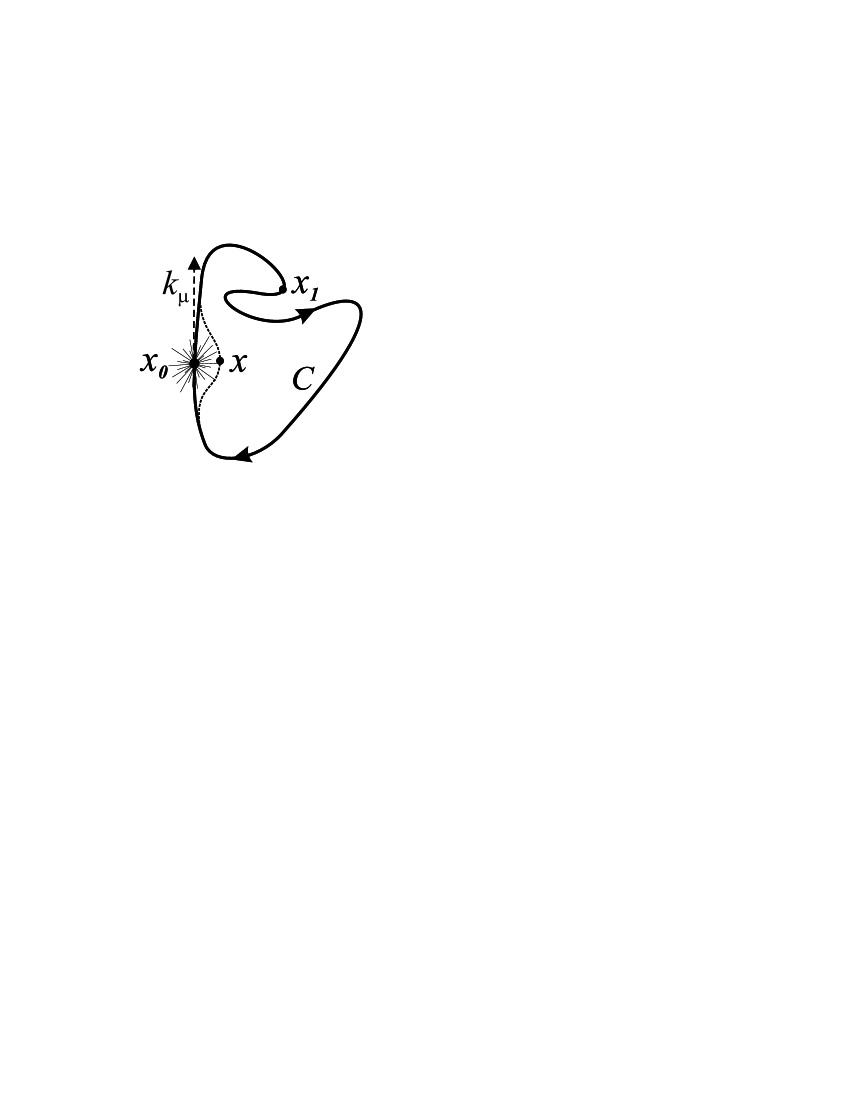
Figure 1: The contour ${\cal C}$ (solid line) and its variation (dotted line) used in definition of the monopole.

To make a rigorous definition of an object associated with the trajectory ${\cal C}$, let us study an untraced Wilson loop which starts and ends at some point $x_{0}\in{\cal C}$:

$$W_{\cal C}(x_{0})=P\,\exp\Bigl{\{}ig\,\oint_{{\cal C}}{\mathrm{d}}x_{\mu}\,A_{\mu}(x)\Bigr{\}}\,.$$ (15)

This operator transforms under the gauge transformations as an adjoint operator, similarly to the operator $X$, Eq. (1). To make an analogy with $X$ closer, we subtract the singlet part from (15), defining another adjoint operator:

$$\Gamma_{\cal C}(x_{0})=W_{\cal C}(x_{0})-{\mathchoice{\rm 1\mskip-4.0mul}{\rm 1\mskip-4.0mul}{\rm 1\mskip-4.5mul}{\rm 1\mskip-5.0mul}}\cdot\frac{1}{2}\,{\mathrm{Tr}}\,W_{\cal C}(x_{0})\,.$$ (16)

By the construction, the operator $\Gamma$ is traceless, and under the gauge transformations it behaves as follows $\Gamma_{\cal C}(x_{0})\to\Omega^{\dagger}(x_{0})\Gamma_{\cal C}(x_{0})\Omega(x_{0})$.

The gauge-invariant condition for our object to have the loop ${\cal C}$ as its world-line trajectory, is to require that the untraced Wilson loop (15) belongs to the center of the group, $W_{\cal C}(x_{0})\in{Z\!\!\!Z}_{2}$. Then the matrix $\Gamma_{\cal C}$ vanishes,

$$\mbox{Condition 1}:\qquad W_{\cal C}(x_{0})=\pm{\mathchoice{\rm 1\mskip-4.0mul}{\rm 1\mskip-4.0mul}{\rm 1\mskip-4.5mul}{\rm 1\mskip-5.0mul}}\qquad\Leftrightarrow\qquad\Gamma_{\cal C}(x_{0})=0\,.$$ (17)

This condition is gauge invariant since the eigenvalues of the Wilson loop are gauge invariant quantities. Equation (17) is very similar to Eq. (3) which appears in the ’t Hooft construction. The matrix $\Gamma$ plays the role of the diagonalization matrix $X$. The condition (17) is required but not sufficient criterium for our object to have the loop ${\cal C}$ as its world-line trajectory.

The condition (17) is self-consistent in a sense, that if the matrix $\Gamma$ vanishes at the point $x_{0}$, then it also vanishes at any other point along the trajectory ${\cal C}$. To show this, let us consider an arbitrary point $x_{1}$ at the contour ${\cal C}$, Figure 1. Then the Wilson loops (15) open at the points $x_{0}$ and $x_{1}$ are related to each other by the adjoint transformation:

$$W_{\cal C}(x_{1})=U^{\dagger}(x_{1},x_{0})\,W_{\cal C}(x_{0})\,U(x_{1},x_{0})\,,\qquad U(x_{1},x_{0})=P\,\exp\Bigl{\{}ig\,\oint^{x_{1}}_{x_{0}}{\mathrm{d}}x_{\mu}\,A_{\mu}(x)\Bigr{\}}\,.$$ (18)

Obviously, if $W_{\cal C}(x_{0})\in{Z\!\!\!Z}_{2}$ then $W_{\cal C}(x_{1})\in{Z\!\!\!Z}_{2}$ as well, and, consequently, $\Gamma_{\cal C}(x_{1})\equiv 0$. Thus the condition (17) is in fact independent on the reference point $x_{0}$.

In order to show that the simple condition (17) does indeed have a similarity with the monopole, let us deform infinitesimally the contour ${\cal C}\to{\cal C}^{\prime}={\cal C}+\delta{\cal C}$ in the vicinity of the point $x_{0}$, Figure 1. After the deformation the point $x_{0}$ is shifted to the new location $x$ (for the sake of simplicity we do not further use the prime symbol in ${\cal C}^{\prime}$). The infinitesimal deformations in the tangent direction to the current $k_{\mu}(x_{0})$ should not change value of $\Gamma_{\cal C}$ as we have just seen. Therefore a non-trivial variation should only be done in the direction, perpendicular to $k_{\mu}(x_{0})$. Without loss of generality let us assume that the current is $k_{\mu}\propto\delta_{\mu,4}$ and then the infinitesimal vector $x-x_{0}$ should only have spatial non-zero components.

In general case the deformed loop $\Gamma_{\cal C}(x)$ should have a hedgehog-like structure in the vicinity of the zero-point $x_{0}$,

$$\mbox{Condition 2}:\qquad\Gamma_{\cal C}(x)=\frac{\sigma^{a}}{2}\,{\cal Y}^{ai}_{\cal C}{\bigl{(}x-x_{0}\bigr{)}}^{i}+O\Bigl{(}\bigl{(}x-x_{0}\bigr{)}^{2}\Bigr{)}\,,$$ (19)

where ${\cal Y}$ matrix is similar to the matrix $Y$ of Eq. (4). This is the second condition for a hedgehog–like object to be located at point $x_{0}$. One may interpret our construction in terms of the Abelian monopoles which appear in the Abelian gauge formalism. The diagonalization of the Wilson loop $W_{\cal C}$ corresponds to a ”dynamical Abelian gauge”. If the eigenvalues of the loop $W_{\cal C}$ coincide, and the hedgehog structure (20) appears, then we have in this dynamical Abelian gauge the singularity on the trajectory ${\cal C}$.

Note that Condition 1 follows from Condition 2, while the opposite is not valid in general. The situation is quite similar to the Abrikosov vortex solution in the Ginzburg-Landau model: in the center of the vortex the scalar field is zero (analogously to Condition 1). However, not all zeros of the scalar fields are vortices since the singular behavior of the phase of the scalar field is required as well (an analog of Condition 2). Similarly to our case, the singular phase of the Higgs field guarantees the vanishing of the scalar field in the center of the vortex while the opposite is not generally correct.

As we have seen, Condition 1, Eq. (17), is self-consistent in a sense, that is it fulfilled in any point $x_{0}$ of the loop ${\cal C}$ for isolated ”singularities”. A similar statement should be valid in general case for Condition 2, Eq. (19). Indeed, as we travel along the loop, the hedgehog condition (19) may cease to be valid provided the matrix ${\cal Y}^{ai}_{{\cal C}}$ becomes degenerate at some point $x_{s}$ of the loop ${\cal C}$, $\mathrm{det}{\cal Y}_{\cal C}(x_{s})=0$. However, the degeneracy means that the singularity is no more isolated, contradicting the initial assumption.

Note, that formally the matrix ${\cal Y}_{\cal C}$ introduced in Eq. (19) may be defined as a variation of the loop ${\cal C}$:

$${\cal Y}^{ai}_{\cal C}(x)=\frac{\delta\Gamma_{\cal C}^{a}(x)}{\delta x^{i}}{\Biggl{|}}_{x\to x_{0}}\,,\qquad a,i=1,2,3\,.$$ (20)

This equation is very similar to Eq. (4) with the only exception: instead of the usual derivative, in the definition of the matrix ${\cal Y}_{\cal C}$ we have formally used the path derivative $\delta$ which defines a change of the functional $\Gamma_{\cal C}$ under the infinitesimal change of the contour ${\cal C}$. The variation itself is infinitesimally small, since the change in the loop functional $W_{\cal C}$ is proportional to the area of the loop variation.

In a Lorentz–invariant form the matrix ${\cal Y}_{\cal C}$ can be written as follows:

$${\cal Y}^{a\nu}_{\cal C}(x)\propto m^{\mu}_{\cal C}\,F^{a}_{\mu\nu}\,,$$ (21)

where we took into account Eq. (17). Here $m^{\mu}_{\cal C}(x)=\dot{x}^{\mu}_{\cal C}/|\dot{x}_{\cal C}|$ is tangent vector to the contour ${\cal C}$, where $\dot{x}^{\mu}_{\cal C}\equiv\partial{\bar{x}}^{\mu}_{\cal C}(\tau)/\partial\tau$, and the contour ${\cal C}$ is parameterized by the vector function ${\bar{x}}^{\mu}_{\cal C}$ of the variable $\tau$. Thus, if

$${\mathrm{d}et}_{\perp}\bigl{(}m^{\mu}_{\cal C}\,F^{a}_{\mu\nu}\bigr{)}\neq 0\,,$$ (22)

then we have a hedgehog around the curve defined by the condition (17). The determinant is taken over indices $a$ and $\nu$, where the index $\nu$ is running in the 3D Lorentz subspace perpendicular to the tangent vector $m^{\mu}_{\cal C}$.

The hedgehog singularity has something to do with electric fields rather than with the magnetic ones. Indeed in the case of a static trajectory the matrix (21) becomes a chromoelectric field, $E^{a}_{i}\equiv F^{a}_{4i}$. Therefore it is difficult to associate the discussed objects with magnetic monopoles despite the Abelian monopole construction was explicitly used to define the objects. The structure of the gluon fields of the object is dual to the structure of the ’t Hooft-Polyakov monopoles which possesses a hedgehog in the chromomagnetic sector.

One the other hand, it is clear that these hedgehogs should be related in one or in another way to the confinement properties of the system because their construction is done entirely in terms of the Wilson loops (and, as it is well-known, the expectation value of the Wilson loop variable is tightly related to the confinement property of the Yang-Mills theory). The static hedgehogs should be sensitive to the deconfinement phase transition since this transition marks a change in the behavior of the electric components of the gluon fields.

We expect that the physics of these objects is non-perturbative, which can be uncovered, for example, by a numerical lattice simulation which is one of the most powerful non-perturbative methods. Unfortunately, a non-local definition of the hedgehogs makes it difficult to locate this object in a given configuration of the (lattice) gluon field. Moreover, a chance to find this object directly in a lattice regularization is almost zero since the Wilson loop is unlikely to be precisely center-valued. Loosely speaking, the hedgehog goes through the meshes of the lattice and it seems that the individual hedgehog is difficult to locate. However, one can overcome this principal difficulty by studying statistical rather than individual properties of the hedgehogs. For example, in the SU(2) gauge theory one can study a distribution $D_{\cal C}(\omega)=\langle\delta(W_{\cal C}-\omega)\rangle$ of the trace of the Wilson loop $W_{\cal C}$ at a trajectory of a fixed shape ${\cal C}$. The distribution is to be evaluated at the gluon field ensemble. Then the density of the center values of the Wilson loop $W_{\cal C}$ can be obtained by an extrapolation of the distribution $D_{\cal C}(\omega)$ to the center values, $w\to\pm 1$. It is clear that such limiting values are in a general case finite quantity despite the center value $W_{\cal C}=\pm 1$ itself can not be reached exactly in the lattice simulations. These distributions should provide information on the density, correlation functions and other properties of these objects.

IV Examples

IV.1 Vacuum configuration

Consider the trivial vacuum configuration $A^{a}_{\mu}=0$. In this case all untraced Wilson loops are belonging to the center of the group, $W_{\cal C}\equiv{\mathchoice{\rm 1\mskip-4.0mul}{\rm 1\mskip-4.0mul}{\rm 1\mskip-4.5mul}{\rm 1\mskip-5.0mul}}$. However, the hedgehog structure cannot obviously be found in the vicinity of any of these contours. Thus, despite Condition 1, Eq. (17), is fulfilled, Condition 2, Eq. (19), is not: the trivial configuration gives no singularities according to our criteria.

IV.2 BPS monopole

The self-dual BPS monopole solution ref:BPS to the SU(2) Yang–Mills equation of motion is

$$A^{a}_{i} = \frac{1}{g}\,f(r)\varepsilon_{iab}n^{b}\,,\qquad f(r)=\frac{1}{r}\Bigl{(}1-\frac{r}{\sinh r}\Bigr{)}\,,$$ (23)

$$A^{a}_{4} = \frac{1}{g}\,h(r)\,n^{a}\,,\qquad\hskip 14.22636pth(r)=\frac{1}{r}\Bigl{(}r\coth r-1\Bigr{)}\,,$$ (24)

where $n^{a}=x^{a}/|x|$, and $r\equiv|x|$ is assumed to be scaled by an arbitrary factor, $r\to r_{0}\cdot r$, to make a dimensionless quantity. The solution is static and self-dual. The hedgehog configuration may only be present in the vicinity of the monopole, ${\mathbf{x}}=0$. Since the monopole is anyway static, let us consider the periodic boundary conditions: the time direction is assumed to be compactified to a circle with the length $T$.

Consider an untraced Wilson loop which coincides with an untraced Polyakov loop,

$${\cal P}_{\cal C}(x)\equiv W_{\cal C}(x)=W(x_{0},B)\cdot W(B^{\prime},x_{0})\,,\qquad W(x,y)\equiv P\exp\Bigl{\{}ig\int_{x}^{y}{\mathrm{d}}x_{\mu}\,A_{\mu}\Bigr{\}}\,,$$ (25)

where integrations are taken along the straight contour ${\cal C}$ parallel to the time direction, Figure 2.

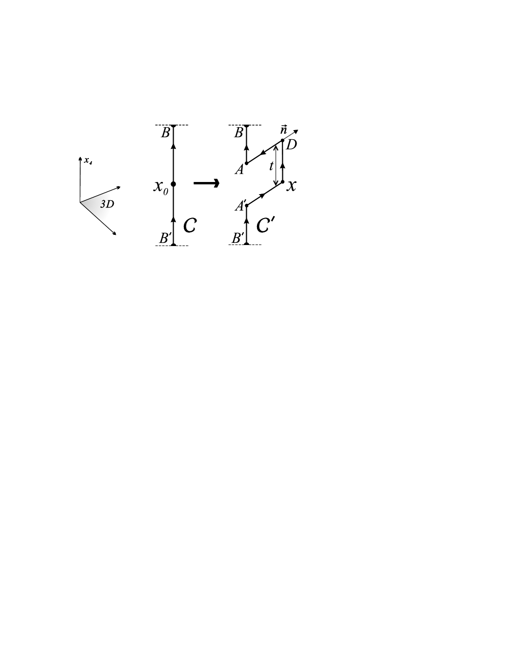
Figure 2: The contours used as probes for the BPS monopole.

Due to periodic boundary conditions the matrix ${\cal P}_{\cal C}(x)$ in Eq. (25) transforms as an adjoint operator. Using Eq. (24) one can easily see that the condition (17) is fulfilled at the point ${\mathbf{x}}=0$ as well as at the spheres $r=r_{n}$ with $Th(r_{n})=2\pi n$, $n\in{Z\!\!\!Z}$. One can easily show that at the spheres $r=r_{n}$ due to the absence of the isolated singularities the hedgehog condition (19) is not fulfilled. Therefore below we consider the point ${\mathbf{x}}=0$ only.

We deform the contour ${\cal C}\to{\cal C}^{\prime}$ as it is shown in Figure 2. Since $A_{4}({\mathbf{x}}=0)=0$ and the points $A$, $A^{\prime}$, $B$ ad $B^{\prime}$ are located at ${\mathbf{x}}=0$ line, then $W(B^{\prime},A^{\prime})=W(A,B)={\mathchoice{\rm 1\mskip-4.0mul}{\rm 1\mskip-4.0mul}{\rm 1\mskip-4.5mul}{\rm 1\mskip-5.0mul}}$. Due to the structure of the spatial components of the gluon field (23) we have $W(A^{\prime},x)=W(D,A)={\mathchoice{\rm 1\mskip-4.0mul}{\rm 1\mskip-4.0mul}{\rm 1\mskip-4.5mul}{\rm 1\mskip-5.0mul}}$. Finally, we find that the only nontrivial element of the path is $xD$, and we get (taking $t\to 0$ and $r\to 0$):

$${\cal P}_{{\cal C}^{\prime}}(x) = {\mathchoice{\rm 1\mskip-4.0mul}{\rm 1\mskip-4.0mul}{\rm 1\mskip-4.5mul}{\rm 1\mskip-5.0mul}}\cdot\cos h(r)t/2+i\sigma^{a}n^{a}\cdot\sin h(r)t/2={\mathchoice{\rm 1\mskip-4.0mul}{\rm 1\mskip-4.0mul}{\rm 1\mskip-4.5mul}{\rm 1\mskip-5.0mul}}+i\frac{t}{6}\cdot\sigma^{a}x^{a}+O(t^{2},r^{2})\,,$$ (26)

$$\Gamma_{{\cal C}^{\prime}}(x) = i\frac{t}{6}\cdot\sigma^{a}x^{a}+O(t^{2},r^{2})\,.$$ (27)

Thus, we obtain that condition 2, Eq. (19), is fulfilled at ${\mathbf{x}}=0$. The matrix ${\cal Y}_{\cal C}$, Eq. (20), is an infinitesimally small matrix proportional to a unit matrix. The determinant of ${\cal Y}_{\cal C}$ is non–zero, thus we have clearly a non-degenerate case. Therefore, for the self-dual BPS monopole configuration our construction of the hedgehog gives the correct location of the monopole center. Technically, our definition of the gauge-invariant object, has identified the hedgehog-like structure of the chromoelectric components of the self-dual BPS monopole.

IV.3 Polyakov Abelian gauge

The Polyakov Abelian gauge is defined by the diagonalization of (untraced) Polyakov loops $P_{\cal C}(x)$, Eq. (25). The isolated Abelian monopoles in this gauge are always static. The Polyakov gauge has analytically been considered in Refs. ref:Yukawa ; ref:Polyakov:gauge ; ref:Jahn . The monopole positions are located by conditions (3) and (4) in which the operator $X$ is identified with ${\cal P}_{\cal C}(x)$. The Polyakov-loop variable can also be used to find (static) monopole constituents in physically interesting topologically non-trivial configurations ref:Falk . The static BPS configuration in the Polyakov Abelian gauge corresponds to an Abelian monopole. Thus, our recipe determines the monopole position in the Polyakov gauge correctly if the background configuration is the BPS monopole or the like. However, in a case of a general configuration our construction and the definitions for an Abelian monopole in the Polyakov Abelian gauge may give different results.

IV.4 Dynamics at finite temperature

At a finite temperature the Euclidean space-time is compactified in one of the directions (it is called ”imaginary time”, or ”temperature” direction). As the temperature increases, the length of the compactified direction becomes shorter and the gauge field is forced to be static. This immediately implies, that our objects – located by conditions (17,19) – must also become more and more static as temperature gets higher. Indeed, if the object moves along a spatial direction at a point $x$, then the gauge field must evolve in the temporal direction to support the hedgehog structure (19). However, the evolution of the fields in the temporal direction – and, therefore, the motion of the object in a spatial direction – is suppressed at high temperatures.

Moreover, at low temperatures ($i.e.$, in the confinement phase) the distribution of the values of the Polyakov lines is peaked around $(1/2)\,{\mathrm{Tr}}{\cal P}(x)=0$ value, while at high temperatures the Polyakov loops tend to be concentrated near $(1/2)\,{\mathrm{Tr}}{\cal P}(x)=\pm 1$ values supporting condition 1, Eq. (17). The described behavior of the Polyakov lines indicates that as the temperature increases the density of static objects becomes higher and higher compared to the density of the spatial currents. Similar property is observed for the Abelian monopoles in lattice simulations ref:finite:T .

IV.5 Lower dimensions

In lower dimensions the similar object can also be formally defined by condition 1. However, the hedgehog condition (19) can not be fulfilled since there is no hedgehog structure (in a monopole sense) around the trajectory ${\cal C}$ in two spatial dimensions. This consideration means that the hedgehog structure around the object should be of the chromoelectric nature.

V Discussion and Conclusion

We propose a gauge–invariant definition of a hedgehog-like object in non-Abelian gauge models. The trajectory of this object is a closed curve defined by the requirement for the (untraced) Wilson loop to take its value in the center of the color group. This definition shares similarities with ’t Hooft definition of an Abelian monopole and locates correctly the trajectory of the self-dual BPS monopole. One the other hand, the hedgehog-like behavior is encoded in the chromoelectric components of the gluon field, implying that the hedgehogs should be sensitive to the finite temperature phase transition. We provided arguments that the density of the static hedgehogs should increase with the rise of temperature.

It is interesting to check the properties of these objects on the lattice despite the lattice definition of an individual hedgehog in a configuration of the gluon fields is somewhat obscure. We have proposed a method to implement our construction by studying statistical rather than individual properties of the hedgehogs with the help of distributions of the Wilson loops and/or their eigenvalues at trajectories of fixed shapes.

- (1) Y. Nambu, Phys. Rev. D 10, 4262 (1974); G. ’t Hooft, in High Energy Physics, ed. A. Zichichi, EPS International Conference, Palermo (1975); S. Mandelstam, Phys. Rept. 23, 245 (1976).
- (2) T. Suzuki, Nucl. Phys. Proc. Suppl. 30, 176 (1993); M. N. Chernodub, M. I. Polikarpov, “Abelian projections and monopoles”, in ”Confinement, duality, and nonperturbative aspects of QCD”, Ed. by P. van Baal, Plenum Press, p. 387, hep-th/9710205 (1997); R.W. Haymaker, Phys. Rept. 315, 153 (1999).
- (3) G. ’t Hooft, Nucl. Phys. B190, 455 (1981).
- (4) M. N. Chernodub, F. V. Gubarev, M. I. Polikarpov and A. I. Veselov, Prog. Theor. Phys. Suppl. 131, 309 (1998).
- (5) M. N. Chernodub, Phys. Rev. D 69, 094504 (2004).
- (6) A. S. Kronfeld, M. L. Laursen, G. Schierholz and U. J. Wiese, Phys. Lett. B198, 516 (1987).
- (7) T. Suzuki and I. Yotsuyanagi, Phys. Rev. D42, 4257 (1990).
- (8) M. N. Chernodub, F. V. Gubarev, M. I. Polikarpov and V. I. Zakharov, Nucl. Phys. B 592, 107 (2001); ibid. 600, 163 (2001).
- (9) F. V. Gubarev and V. I. Zakharov, Int. J. Mod. Phys. A 17, 157 (2002); hep-lat/0204017; F. V. Gubarev, hep-lat/0204018.
- (10) P. Skala, M. Faber and M. Zach, Nucl. Phys. B 494, 293 (1997).
- (11) T. Suzuki, K. Ishiguro, Y. Mori and T. Sekido, Phys. Rev. Lett. 94, 132001 (2005).
- (12) F. V. Gubarev, L. Stodolsky and V. I. Zakharov, Phys. Rev. Lett. 86, 2220 (2001).
- (13) A. Kovner, M. Lavelle and D. McMullan, JHEP 0212, 045 (2002).
- (14) F. V. Gubarev and V. I. Zakharov, hep-lat/0211033.
- (15) A. S. Kronfeld, G. Schierholz and U. J. Wiese, Nucl. Phys. B 293, 461 (1987); H. Suganuma, S. Sasaki and H. Toki, Nucl. Phys. B 435, 207 (1995).
- (16) G. ’t Hooft, Nucl. Phys. B 79, 276 (1974).
- (17) A. M. Polyakov, JETP Lett. 20, 194 (1974).
- (18) J. Arafune, P. G. O. Freund and C. J. Goebel, J. Math. Phys. 16, 433 (1975).
- (19) O. Jahn and F. Lenz, Phys. Rev. D 58, 085006 (1998); O. Jahn, J. Phys. A 33, 2997 (2000).
- (20) E. B. Bogomolny, Sov. J. Nucl. Phys. 24, 449 (1976); M. K. Prasad and C. M. Sommerfield, Phys. Rev. Lett. 35, 760 (1975); P. Rossi, Phys. Rept. 86, 317 (1982).
- (21) M. Garcia Perez, A. Gonzalez-Arroyo, A. Montero and P. van Baal, JHEP 9906, 001 (1999); F. Bruckmann, D. Nogradi and P. van Baal, Acta Phys. Polon. B 34, 5717 (2003); F. Bruckmann, E. M. Ilgenfritz, B. V. Martemyanov and P. van Baal, Phys. Rev. D 70, 105013 (2004).
- (22) S. Ejiri, S. I. Kitahara, Y. Matsubara and T. Suzuki, Phys. Lett. B 343, 304 (1995); S. I. Kitahara, Y. Matsubara and T. Suzuki, Prog. Theor. Phys. 93, 1 (1995); S. Ejiri, Phys. Lett. B 376, 163 (1996).