Quarkonium correlators and spectral functions at zero and finite temperature from Fermilab action

Abstract

We study charmonium and bottomonium systems at zero and finite temperatures using Lattice QCD with Fermilab action on anisotropic lattices.

1 Introduction

There has been considerable progress in studying quarkonium properties at finite temperature since the work of Matsui and Satz MS86 . In the past the quarkonium properties at finite temperature were studied in potential models karsch88 ; digal01a ; digal01b (for recent works see Refs. shuryak04 ; wong04 ). The applicability of the potential models at finite temperature is not obvious petreczkythis . It is more appropriate to study the in-medium modifications of meson properties at finite temperature in terms of spectral functions (for recent review see rapp ; petreczky03 ; Karsch:2003jg ; petreczkylat04 ). Meson correlators in Eucledian time have been calculated in Lattice QCD for a long time, but to get spectral functions out of them was considered impossible. However it was shown by Asakawa, Hatsuda and Nakahara that using the Maximum Entropy Method one can in principle reconstruct also meson spectral functions. The method was successfully applied at zero temperature asakawa01 ; cppacs and later also at finite temperature karsch02 ; wetzorke02 ; karsch03 ; asakawa04 ; datta04 ; asakawa02 ; umeda02 ; wetzorke03 . Though systematic uncertainties in the spectral function calculated on lattice are not yet completely understood, it was shown in Ref. karsch02 ; datta04 that a precise determination of the imaginary time correlator can alone provide stringent constraints on the spectral function at finite temperature.

2 Lattice setup and simulation details

We simulate both bottomonium and charmonium using the so called Fermilab action Fermilab . It is a special formulation of the O(a) improved Wilson action with broken axis-interchange symmetry: time-like and space-like coefficients are treated independently and are determined in a non-perturbative way using the dispersion relation. This formulation is known to significantly reduce lattice artefacts at modest lattice spacings. As our major interest lies at finite temperature theory we face the problem of time extent being very short, which makes it difficult to fit the correlators. Therefore, following chen01 ; Manke we introduce anisotropic lattice, setting $a_{s}/a_{t}=\xi\neq 1$.

Such calculations require immense computational power, as to resolve ground state from excited state we need small lattice spacing. One of the ways to address this problem is building a dedicated Lattice QCD machine such as QCDOC. This supercomputer was developed by physisists from Columbia University, BNL, RIKEN and UKQCD. Three such machines, each reaching about 10TFlops peak performance, are currently under construction at BNL and EPCC. We used for our simlations QCDOC prototypes, single-motherboard machines at about 50 GFlops peak. Such resources are still not adequate for the full QCD simulations, so we use quenched approximation, which is equivalent to neglecting quark loops. Typical statistics gathered was 500 to 1000 measurements, separated by 400 updates.

To study meson properties at finite temperature one considers the following correlators of some operator $\hat{O}$

$$D^{>}(t,t^{\prime})=\langle\hat{O}(t)\hat{O}(t^{\prime})\rangle_{T},~{}~{}~{}D^{<}(t,t^{\prime})=\langle\hat{O}(t^{\prime})\hat{O}(t)\rangle_{T},$$ (1)

where $\langle...\rangle_{T}=\langle...e^{-\hat{H}/T}\rangle_{T}$ denotes the thermal average lebellac . As we cannot do any lattice simulation in Minkowski space we need to introduce a Wick rotation and we get the imaginary time correlator

$$G(\tau)=\langle\mathcal{T}\hat{O}(-i\tau)\hat{O}(0)\rangle.$$ (2)

(where $\mathcal{T}$ denotes time ordering). Now we define a spectral function through the Fourier transform of $D^{>(<)}(t)$ as

$$\sigma(\omega)=\frac{D^{>}(\omega)-D^{<}(\omega)}{2\pi}=\frac{1}{\pi}ImD_{R}(\omega),$$ (3)

where $D_{R}(\omega)$ is the retarded correlator. With the help of the KMS condition on $D^{>(<)}$ lebellac we arrive at the following integral relation between the imaginary time correlator and the spectral function

$$\displaystyle G(\tau)=\int_{0}^{\infty}d\omega\sigma(\omega)\frac{\cosh(\omega(\tau-1/2T)}{\sinh\frac{\omega}{2T}}$$

$$\displaystyle\equiv\int_{0}^{\infty}d\omega\sigma(\omega)K(\omega,\tau)$$ (4)

Now we can try to reconstruct the spectral function by calculating $G(\tau)$ on the lattice; however a set of complications arises: At zero temperature the kernel $K(\omega,\tau)$ reduces to simple exponential and when we consider large Euclidean times we only see the contribution from the lowest lying meson state in $\sigma(\omega)$, i.e $G(\tau)=\exp(-m\tau)$. However at finite temperature the time interval is limited and excited states are as important as the ground state. Additional problems arise in lattice calculations where correlators are calculated only on a discrete set of Euclidean times $\tau T=k/N_{\tau}$, $k=0,...,N_{\tau}-1$ with $N_{\tau}$ being the temporal extent of the lattice. In order to reconstruct the spectral functions from this limited information it is necessary to include in the statistical analysis of the numerical results also prior information on the structure of $\sigma(\omega)$ (e.g. such as $\sigma(\omega)>0$ for $\omega>0$). This can be done in many ways, none of them being rigorous. Therefore we use two of such methods, namely the Maximum Entropy Method (MEM) nakahara99 ; asakawa01 and constrained curve fitting lepage . These two methods are totally different both in their assumptions and the procedures and we use them to cross-check our results.

To do a lattice study of particles with given quantum numbers we must produce an appropriate set of operators with given symmetry properties. One such set is a local meson operator which is bilinear in quark-antiquark fields (current) asakawa01 ; cppacs ; karsch02 ; wetzorke02

$$O_{H}(\tau,\vec{x})=\bar{q}(\tau,\vec{x})\Gamma_{H}q(\tau,\vec{x}),~{}~{}~{}\Gamma_{H}=1,\gamma_{5},\gamma_{\mu},\gamma_{5}\gamma_{\mu}$$ (5)

for scalar, pseudoscalar, vector and axial vector channels correspondingly. The pseudo-scalar and vector correlators correspond to ground state quarkonia $\eta_{c,b}(^{1}S_{0})$ and
$J/\psi,\Upsilon(^{3}S_{1})$ respectively. The scalar and axial-vector channels correspond to P state quarkonia, $\chi_{c,b}(J=0,1)$. The temporal correlators at finite spatial momentum $\vec{p}$ then take the following form

$$G_{H}(\tau,\vec{p})=\langle O_{H}(\tau,\vec{p})O_{H}^{\dagger}(\tau,-\vec{p})\rangle,$$

$$O(\tau,\vec{p})=\sum_{\vec{x}}e^{i\vec{p}\vec{x}}O_{H}(\tau,\vec{x})$$ (6)

3 Charmonium at zero and finite temperature

We start the discussion of the numerical results with zero temperature spectral functions in the vector channel. In Fig. 1 we show the spectral functions at four different lattice spacings $a_{t}^{-1}=1.9,~{}2.9,~{}4.0$ and $8.2$ GeV. The anisotropy $\xi=2$ for the first three lattice spacing and $\xi=4$ for the last one. The lattice spacing was fixed using the heavy quark potential and the value of $r_{0}=0.5$ fm for the Sommer scale (see chen01 for further details). As one can see from the figure the first peak, which corresponds to the $J/\psi$ state, does not move as we vary the lattice spacings. On the contrary, the position of the other peaks depends on the lattice spacing. Moreover, as we go to finer lattices more peaks appear. Similar results were obained also in other channels. Thus, all the structures except the first peak cannot be identified with physical states. It is possible that these peaks in fact belong to the continuum distorted by effects of finite lattice. In any case this problem requires further analysis which will be presented elsewhere self . We also analyzed the spectral functions using constrained curve fitting by using a multi-exponential Ansatz with four or more terms. The results from the fits are shown in Fig.1. For the ground state we get very good agreement between MEM and constrained fit, while it becomes worse for higher states. Nonetheless, the rough agreement between the two methods gives us some confidence as well as indicating the size of possible systematic errors.

Figure 1: The zero temperature vector spectral function for charmonium at different lattice spacings (top). Also shown the vector spectral function at $a_{t}^{-1}=4$GeV compared with the results of constrained curve fit (vertical lines).

Now we are in a position to discuss spectral functions at finite temperature. For $a_{t}^{-1}=8.2$ GeV we have sufficient number of data points for temperatures above deconfinement to analyze the spectral function. In Fig.2 the spectral function in pseudo-scalar and scalar channel is shown. The peak corresponding to $\eta_{c}$ state survives in the plasma phase; moreover, its position is essentially unchanged. This is consistent with previous findings asakawa04 ; datta04 ; umeda02 . The scalar channel has been analyzed only in Ref.datta04 and it was found that the $\chi_{c}$ state dissolves in the plasma soon after the deconfinement temperature. The analysis of the scalar spectral function shown in Fig.2 confirms this conclusions.

Figure 2: The charmonia spectral functions for $a_{t}^{-1}=8.2$ GeV at zero temperature and above deconfinement temperature $T=1.1T_{c}$ corresponding to $N_{t}=24$.

4 Bottomonium spectral functions and correlators

While charmonium has been studied by other collaborations, the bound states of $b$-quarks received much less attention. In fact this is the first study of the bottomonium at finite temperature. As in the charmonium case we start with zero temperature physics. The bottominium spectrum using Fermilab action was studied in Ref. Manke where extened meson operators have been used. We have studied the bottomonium spectrum using two lattice spacings $a_{t}^{-1}=8.2$GeV and $a_{t}^{-1}=12.0$GeV and $\xi=4$ estimated from the Sommer scale. In Fig.3 bottomonia spectral functions in scalar and pseudo-scalar channels are shown. Because of the large bottomonia mass the correlators are quite noisy and we found that it is considerably more difficuilt to reconstruct the spectral functions then it was in the charmonia case.

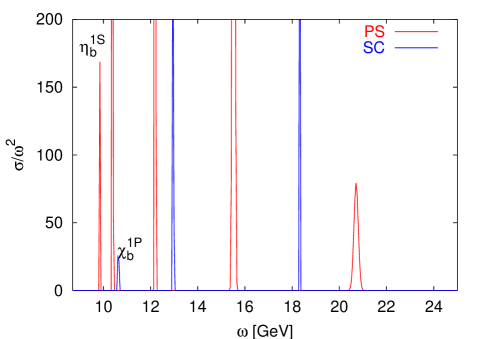
Figure 3: Bottomonium spectral functions at zero temperature, scalar and pseudo-scalar channels for $a_{t}^{-1}=12$GeV.

As the analysis of the bottomonium spectral functions is difficuilt already at zero temperature at finite temperature we study only the temperature dependence of the correlator. This method is based on the following argument datta04 : in Eq.4 the temperature dependence of the right hand side comes from two sources - the spectral function itself and the finite temperature kernel. Now let us introduce the so-called reconstructed correlator using the spectral function at zero temperature

$$G_{recon}(\tau,T)=\int_{0}^{\infty}d\omega\sigma(\omega,T=0)\frac{\cosh(\omega(\tau-1/(2T))}{\sinh\frac{\omega}{2T}}.$$ (7)

If the spectral function does not depend on temperature then the reconstructed and directly calculated correlators will be equal, i.e. $G(\tau,T)/G_{recon}(\tau,T)=1$. We show their ratio for the pseudo-scalar channel ($S-wave$) and the scalar channel ($P-wave$) of the bottomonium on Fig.4. As one can see there is no modification of the correlator for the $\eta_{b}$ particle till almost twice the critical temperature. However, quite suprisingly, for the $\chi_{b}$ we see a drastic change already at $1.3T_{c}$ which suggests that something has happened. The $\chi_{b}$ state has approximately the same size and binding energy as the $J/\psi$ or $\eta_{c}$ state which do not show any change till $(1.7-2.0)T_{c}$. Thus we would expect the same for $\chi_{b}$. It also is possible that the large change in the scalar correlator is not caused by the dissolution of the $\chi_{b}$ but rather by modification of the continuum part of the spectral function mocsy .

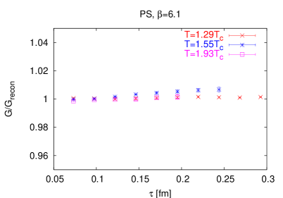
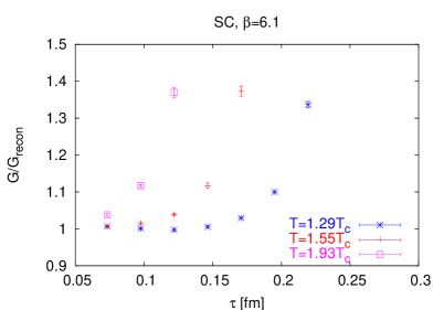
Figure 4: The ratio $G(\tau,T)/G_{recon}(\tau,T)$ at different temperatures for pseudo-scalar (top) and scalar (bottom) correlators.

5 Conclusions and Outlook

We analysed charmonium and bottomonium systems at zero and finite temperatures using Lattice QCD with Fermilab action on anisotropic lattices. We reconstructed their spectral functions, reliably identifying ground states for various values of the lattice cutoff. The $S-wave$ states in both systems survive in the deconfined phase till as much as three times the critical temperature, while $P-wave$ states may dissolve shortly after the phase transition. The situation with higher excited states, especially $2S$, is very questionable and requires further study.

6 Acknowlegements

This presentation is done based on work in collaboration with P. Petreczky and A. Velytsky and is supported by U.S. Department of Energy under Contract No. DE-AC02-98CH10886 and by SciDAC project. The Maximum entropy method analysis was done using the program developed by A. Jakovác. K.P. would like to thank Kavli ITP at UCSB for the hospitality. Results are obtained on RIKEN/BNL QCDOC prototypes using Columbia Physics System with high-performance clover inverter by P. Boyle and other parts by RBC collaboration. Special thanks to C. Jung for his generous help with CPS.

References

- (1) T. Matsui and H. Satz, Phys. Lett. B 178, 416 (1986).
- (2) F. Karsch, M. T. Mehr and H. Satz, Z. Phys. C 37, 617 (1988).
- (3) S. Digal, P. Petreczky and H. Satz, Phys. Lett. B 514, 57 (2001)
- (4) S. Digal, P. Petreczky and H. Satz, Phys. Rev. D 64, 094015 (2001)
- (5) E. V. Shuryak and I. Zahed, Phys. Rev. D 70, 054507 (2004)
- (6) C. Y. L. Wong, hep-ph/0408020.
- (7) P. Petreczky, hep-lat/0502008 [these proceedings]
- (8) R. Rapp, J. Wambach, Adv. Nucl. Phys. 25, 1 (2000); R. Rapp, L. Grandchamp, hep-ph/0305143
- (9) P. Petreczky, J. Phys. G 30, S431 (2004) [arXiv:hep-ph/0305189].
- (10) F. Karsch and E. Laermann, arXiv:hep-lat/0305025.
- (11) P. Petreczky, arXiv:hep-lat/0409139.
- (12) Y. Nakahara,M. Asakawa and T. Hatsuda, Phys. Rev. D 60, 091503 (1999)
- (13) M. Asakawa,T. Hatsuda, Y. Nakahara, Prog. Part. Nucl. Phys. 46, 459 (2001)
- (14) CP-PACS Collaboration, T. Yamazaki, Phys. Rev. D D65, 014501 (2002)
- (15) F. Karsch et al, Phys. Lett. B530, 147 (2002)
- (16) I. Wetzorke et al, Nucl. Phys. B (Proc. Suppl.) 106, 513 (2002)
- (17) F. Karsch et al, Nucl.Phys. B. A715, 701c (2003)
- (18) M. Asakawa and T. Hatsuda, Phys. Rev. Lett. 92, 012001 (2004) [arXiv:hep-lat/0308034].
- (19) S. Datta, F. Karsch, P. Petreczky and I. Wetzorke, Phys. Rev. D 69, 094507 (2004) [arXiv:hep-lat/0312037].
- (20) M. Asakawa, T. Hatsuda and Y. Nakahara, Nucl. Phys. A 715, 863 (2003) [Nucl. Phys. Proc. Suppl. 119, 481 (2003)] [arXiv:hep-lat/0208059].
- (21) T. Umeda, K. Nomura and H. Matsufuru, arXiv:hep-lat/0211003.
- (22) I. Wetzorke, arXiv:hep-lat/0305012.
- (23) P. Chen, Phys.Rev. D64, 034509 (2001)
- (24) X. Liao and T. Manke, Phys. Rev. D 65, 074508 (2002) [arXiv:hep-lat/0111049].
- (25) A. X. El-Khadra, A. S. Kronfeld and P. B. Mackenzie, Phys. Rev. D 55, 3933 (1997) [arXiv:hep-lat/9604004].
- (26) M. Le Bellac 1996, Thermal Field Theory ( Cambridge University Press )
- (27) G. P. Lepage et al, Nucl. Phys. B ( Proc. Suppl.) 106, 12 (2002)
- (28) S. Gupta, hep-lat/0301006
- (29) P. Petreczky, K. Petrov and A. Velytsky, work in progress
- (30) Á. Mócsy, P. Petreczky, hep-ph/0411262, these proceedings