Non–perturbative improvement of the axial current for dynamical Wilson fermions

Abstract:

A non–perturbative determination of the axial current improvement coefficient $c_{\rm A}$ is performed with two flavors of dynamical improved Wilson fermions and plaquette gauge action. The improvement condition is formulated with Schrödinger functional boundary conditions and enforced at constant physical volume. Large sensitivity is obtained by using two different pseudo–scalar states in the PCAC relation. We estimate the resulting correction to $F_{\rm PS}$ at $\beta=5.2$ to be around $10\%$.

1 Introduction

The approach of lattice observables to their continuum limit can be understood in terms of Symanzik’s effective low energy theory [1, 2]. When applied to QCD with Wilson fermions [3], close to the continuum limit, it predicts that scaling violations are dominated by terms linear in the lattice spacing $a$. These effects can be removed by adding a single term to the action, with properly tuned coefficient $c_{\rm sw}$ [4]. Linear effects in the lattice spacing can also be systematically removed in (on-shell) matrix elements of composite operators [5, 6]. In particular, $\textrm{O}(a)$-improvement of the axial current requires to add one dimension four operator, with coefficient $c_{\rm A}$ (see eq. (3), below). In the quenched approximation, the coefficients $c_{\rm sw}$ and $c_{\rm A}$ have been determined non-perturbatively in the relevant range of bare coupling (or lattice spacings) in [7]. The improvement conditions, which determine the improvement coefficients, were derived from the chiral symmetry of the continuum limit. More precisely, the PCAC relation was required to hold at finite lattice spacing [5, 6, 7]. As will be detailed in sect. 2.2, the PCAC-relation can be considered with different external states. In [5, 6, 7], finite volume states were chosen, formulated in the framework of the Schrödinger functional. Later, $c_{\rm A}$ was also estimated from the PCAC relation in large volume [8, 9] at a couple of values of the lattice spacing. Around $a\approx 0.1$ fm, the results for $c_{\rm A}$ obtained from the finite volume definition [7] differ quite significantly from those obtained in large volume in [8, 9]. At smaller lattice spacing, the difference decreases.

For the interpretation of this difference, one should keep in mind that beyond perturbation theory the improvement coefficients themselves are affected by $\textrm{O}(a)$ ambiguities. In some detail this has been discussed and demonstrated numerically in [10]. The $\textrm{O}(a)$ ambiguity simply corresponds to the fact that the improved theory is treated up to $\textrm{O}(a^{2})$ effects. While this forbids a unique definition of the improved theory, the $\textrm{O}(a)$ ambiguities can be made to disappear smoothly if the improvement condition is evaluated with all physical scales kept fixed, e.g. in units of $r_{0}\approx 0.5\,{\rm fm}$ [11], while only the lattice spacing is varied [10]. We call this the constant physics condition. At the same time one has to take care that the improvement conditions are imposed using low energy states with $E\ll a^{-1}$ since $\textrm{O}(a)$-improvement is valid for those only. So far, the methods of [8, 9] have not yet been implemented such as to satisfy these conditions.

In [12], two improvement conditions for $c_{\rm A}$ were studied, which are easily generalized to respect the above criteria. They are formulated in finite volume with Schrödinger functional boundary conditions, which furthermore helps to render the numerical evaluation feasible in full QCD. We will discuss the improvement conditions briefly in sect. 2.2 and choose one of them to compute $c_{\rm A}$ in the $N_{\rm f}\!=\!2$ theory, where $c_{\rm sw}$ is known from [13, 14]. The knowledge of $c_{\rm A}$ is crucial in order to be able to determine the pseudoscalar decay constants, but also in order to compute renormalized quark masses starting from the PCAC masses, as has been done e.g. in [15, 16].

2 Strategy and techniques

Before going into the details of our strategy and techniques let us comment again on the constant physics condition. In the Schrödinger functional and neglecting the choice of the quark mass for a moment, the relevant point is the following. We need to know how the lattice spacing depends on $\beta$ in order to determine the latter such that a certain $L/a$ corresponds to a prescribed value of $L/r_{0}$. This has to be enforced only with a rather moderate precision, since (sticking with $r_{0}$ as the reference scale) a relative error $\Delta$ in the estimate of $r_{0}/a$ translates into an error of the improvement constant which is proportional to $a/L\!\times\!\Delta$. Thus even if $\Delta$ varies a bit in the considered range of lattice spacings, this is quite irrelevant, in particular if $\Delta$ is a smooth function of the lattice spacing.

In the remainder of this section we will state in more detail how the constant physics condition is implemented. We will also discuss the methods in [7, 12] to determine $c_{\rm A}$, with emphasis on the one we finally used.

2.1 Constant physics condition

With two degenerate flavors of light quarks, the theory has two bare parameters $\beta$ and $m_{0}$. The bare quark mass $m_{0}$ controls the physical quark mass and the bare coupling determines the lattice spacing, defined at vanishing quark mass (for a more precise discussion, which however is of little relevance in this context, see [5, 17]). Non–perturbative estimates of

$$t_{r_{0}}(\beta)=\frac{[r_{0}/a](5.2)}{[r_{0}/a](\beta)}\;,$$ (1)

are available in a limited range of $\beta$ [18, 19]. In [20], the results of [18, 19] were extrapolated to zero quark mass. Taking directly these values for $[r_{0}/a](\beta)$, we have the points with error bars in Fig. 1. From those we roughly estimated the location of the filled points, using the perturbative dependence of the lattice spacing on $\beta$ as a guideline. For our action this is given to three loops in [21], which builds on various steps carried out in [22, 23, 24, 25, 26, 27, 28]. Applied as a pure expansion in the bare coupling (no tadpole improvement), one has

$${a(g_{0}^{2})\over a((g_{0}^{\prime})^{2})} = e^{-[g_{0}^{-2}-(g_{0}^{\prime})^{-2}]/2b_{0}}[g_{0}^{2}/(g_{0}^{\prime})^{2}]^{-{b_{1}/2b_{0}^{2}}}\,\left[\,1+q\,[g_{0}^{2}-(g_{0}^{\prime})^{2}]+{\rm O}\left((g_{0}^{\prime})^{4}\right)\,\right],$$

$$q=0.4529(1)\,,\quad g_{0}<g_{0}^{\prime}\;.$$

The evolution of the lattice spacing relative to our reference point at $(g_{0}^{\prime})^{2}\!=\!6/5.2$ is then expressed by the function $t(\beta)=a(6/\beta)/a(6/5.2)$, which is plotted as a thick line in the graph. It confirms that the filled points are very reasonable choices. Note that other forms of applying bare perturbation theory (differing from eq. (2.1) in the $g_{0}^{4}$-term) would give somewhat different results, but since we are interested in a rather limited range in $g_{0}^{2}$ this does not matter much. Later we will show that systematic uncertainties in $c_{\rm A}$ introduced by this approximate scale setting are negligible.

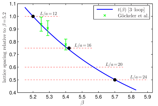
Figure 1: The evolution of the lattice spacing $a$ with the inverse bare gauge coupling $\beta$ from perturbation theory in the lattice scheme and large volume data [18] for the scale $r_{0}$. The filled points correspond to our “scaled” simulations.

Finally, we keep the PCAC mass approximately constant. A precise definition will be given in the following.

2.2 Improvement conditions for the axial current

In this section we discuss criteria for the choice of the improvement condition. With the isovector axial current $A_{\mu}^{a}(x)=\bar{\psi}(x){\textstyle\frac{1}{2}}\tau^{a}\gamma_{\mu}\gamma_{5}\psi(x)$ and the corresponding pseudo–scalar density $P^{a}(x)=\bar{\psi}(x){\textstyle\frac{1}{2}}\tau^{a}\gamma_{5}\psi(x)$ we define the improved axial current [5]

$$(A_{\rm I})_{\mu}^{a}(x)=A_{\mu}^{a}(x)+ac_{\rm A}{\textstyle\frac{1}{2}}(\partial_{\mu}+\partial^{*}_{\mu})P^{a}(x)\;,$$ (3)

where $\partial_{\mu}$ ($\partial_{\mu}^{*}$) denotes the forward (backward) lattice derivative. In the following we will consider quark masses derived from the PCAC relation

$$m(x;\alpha,\beta)=\frac{\langle\alpha|{\textstyle\frac{1}{2}}(\partial_{\mu}+\partial^{*}_{\mu})(A_{\rm I})_{\mu}^{a}(x)|\beta\rangle}{2\langle\alpha|P^{a}(x)|\beta\rangle}\;.$$ (4)

Since this mass is obtained from an operator identity, it is independent of the states $|\alpha\rangle$ and $|\beta\rangle$ as well as the insertion point $x$ up to cutoff–effects. Enforcing this independence at finite lattice spacing leads to possible definitions of improvement conditions [12]. Inserting the expression for the improved current (3) in the previous equation, the quark mass can be written as $m=r+ac_{\rm A}s+\textrm{O}(a^{2})$ with

$$r(x;\alpha,\beta) = \frac{\langle\alpha|{\textstyle\frac{1}{2}}(\partial_{\mu}+\partial^{*}_{\mu})A_{\mu}^{a}(x)|\beta\rangle}{2\langle\alpha|P^{a}(x)|\beta\rangle}$$ (5)

$$\textrm{and}\qquad s(x;\alpha,\beta) = \frac{\langle\alpha|\partial_{\mu}\partial^{*}_{\mu}P^{a}(x)|\beta\rangle}{2\langle\alpha|P^{a}(x)|\beta\rangle}\;.$$ (6)

If we now consider two sets of external states and two insertion points, the improvement condition $m(x;\alpha,\beta)=m(y;\gamma,\delta)$ yields

$$-c_{\rm A}=\frac{\Delta r}{a\Delta s}=\frac{1}{a}\!\cdot\!\frac{r(x;\alpha,\beta)-r(y;\gamma,\delta)}{s(x;\alpha,\beta)-s(y;\gamma,\delta)}$$ (7)

and therefore the sensitivity to $c_{\rm A}$ is given by $a\Delta s$.

Once a reasonably large sensitivity is achieved, all improvement conditions at constant physics are equally valid in the sense that $\textrm{O}(a)$ effects are removed in on-shell quantities. However, the way in which higher–order lattice artifacts are modified will depend on the concrete choice of the improvement condition. In particular, if states with energy not so far from the cutoff are involved, large $\textrm{O}(a^{2})$ effects might be introduced.

We now specialize to Schrödinger functional boundary conditions, introduced in [29, 30] and recall the definition of the relevant correlation functions. One considers QCD in a finite volume $L^{3}\times T$ with Dirichlet boundary conditions in time and periodic boundary conditions in space. More precisely, the fermionic fields are periodic up to a phase $\theta$. By taking functional derivatives with respect to fermionic boundary source fields one can define correlation functions involving the quark fields $\zeta,\overline{\zeta}$ at $x_{0}\!=\!0$ and $\zeta^{\prime},\overline{\zeta}^{\prime}$ at $x_{0}\!=\!T$. In this work we use

$$f_{\rm A}(x_{0};\omega) = -\frac{a^{3}}{3L^{6}}\sum_{\bf x}\langle A_{0}^{a}(x)\,\mathcal{O}^{a}(\omega)\rangle\;,$$ (8)

$$f_{\rm P}(x_{0};\omega) = -\frac{a^{3}}{3L^{6}}\sum_{\bf x}\langle P^{a}(x)\,\mathcal{O}^{a}(\omega)\rangle$$ (9)

$$\textrm{and }\ \ f_{1}(\omega^{\prime},\omega) = -\frac{1}{3L^{6}}\langle\mathcal{O}^{\prime a}(\omega^{\prime})\,\mathcal{O}^{a}(\omega)\rangle$$ (10)

with the pseudo–scalar operator

$$\quad\mathcal{O}^{a}(\omega)=a^{6}\sum_{{\bf x},{\bf y}}\overline{\zeta}({\bf x})\gamma_{5}\tau^{a}{\textstyle\frac{1}{2}}\omega({\bf x}-{\bf y})\zeta({\bf y})$$ (11)

at the $x_{0}\!=\!0$ boundary and the corresponding operator $\mathcal{O}^{\prime a}(\omega^{\prime})$ at the upper boundary of the SF cylinder. These operators depend on spatial trial “wave functions” $\omega$ and $\omega^{\prime}$, respectively.

The Schrödinger Functional version of eqs. (5) and (6) is then given by

$$r(x_{0};\omega) = \frac{{\textstyle\frac{1}{2}}(\partial_{0}+\partial^{*}_{0})f_{\rm A}(x_{0};\omega)}{2f_{\rm P}(x_{0};\omega)}$$ (12)

$$\textrm{and}\qquad s(x_{0};\omega) = \frac{\partial_{0}\partial^{*}_{0}f_{\rm P}(x_{0};\omega)}{2f_{\rm P}(x_{0};\omega)}\;.$$ (13)

To determine $c_{\rm A}$ in the $N_{\rm f}\!=\!0$ theory [7], $\Delta r$ and $\Delta s$ were originally defined through a variation of the periodicity angle $\theta$ of the fermion fields, while keeping $x_{0}\!=\!T/2$ and $\omega\!=\!const$ fixed. For this method the sensitivity $a\Delta s$ is quite low when $L\gtrsim 0.8$fm, $T=2L$. In addition, with dynamical fermions different values of $\theta$ would require separate simulations. We therefore consider this method as too expensive and disregard it in the following. In the quenched approximation two alternatives have been explored in [12].

Requiring the quark mass to be independent of $x_{0}$ (for fixed $\theta$ and $\omega\!=\!const$) is technically easy to implement. However, also in this case the sensitivity is small unless large values of $\theta$ are used. Moreover, the contribution of excited states is not well controlled, because one insertion point must be rather close to a boundary to achieve a sufficiently large sensitivity. Thus energies which are not far removed from the cutoff may contribute.

Secondly, variations of the wave function $\omega$ have been considered. Ideally, one would like to use two wave functions $\omega_{\pi^{(0)}}$ and $\omega_{\pi^{(1)}}$, such that the corresponding operator $\mathcal{O}^{a}(\omega)$ couples only to the ground and first excited state in the pseudo–scalar channel, respectively. As one can easily see from eq. (13) the sensitivity to $c_{\rm A}$ is then proportional to $m_{\pi^{(1)}}^{2}-m_{\pi^{(0)}}^{2}$. Higher excited states are (by definition) not contributing and in principle the method can be used for rather small $T$. Hence, we find this the most attractive method both from a theoretical and practical point of view. In the next section we will detail our approximation to this ideal situation.

2.3 Wave functions

We will now proceed to the more technical aspects of our method. In order to approximate $\omega_{\pi^{(0)}}$ and $\omega_{\pi^{(1)}}$ consider a set of $N$ wave functions. Given a vector $u$ in this $N$–dimensional space, projected correlation functions are defined as $(u,f_{\rm A})$ and $(u,f_{1}u)$, i.e. $f_{\rm A}$ is regarded as a vector and $f_{1}$ as a matrix in this space. It is useful to represent $f_{\rm X}$ ($\rm X=A,P$) and $f_{1}$ as [31]

$$f_{\rm X}(x_{0};\omega_{i}) = \sum_{n=0}^{M-1}F_{\rm X}^{(n)}v_{i}^{(n)}e^{-m_{\pi}^{(n)}x_{0}}+\textrm{O}(e^{-m_{\pi}^{(M)}x_{0}})+\textrm{O}(e^{-m_{\mathrm{G}}(T-x_{0})})\;,$$ (14)

$$f_{1}(\omega_{i},\omega_{j}) = \sum_{n=0}^{M-1}v_{i}^{(n)}v_{j}^{(n)}e^{-m_{\pi}^{(n)}T}+\textrm{O}(e^{-m_{\pi}^{(M)}T})+\textrm{O}(e^{-m_{\mathrm{G}}T})\;,$$ (15)

where $n$ labels the states in the pseudo–scalar channel in increasing energy and $v_{i}^{(n)}$ is the overlap of such a state with the one generated by the action of $\mathcal{O}^{a}(\omega_{i})$ on the SF boundary state. The mass $m_{\mathrm{G}}$ belongs to the lowest excitation in the scalar channel, the $0^{++}$ glueball and the coefficients $F_{\rm X}^{(n)}$ are proportional to the decay constant of the $n$th state. Here we have suppressed the explicit volume dependence of all quantities.

Knowledge of $v^{(n)}$ would allow the construction of vectors $u^{(n)}$, such that – up to corrections of order $e^{-m_{\pi}^{(M)}T}$ – the correlation $(u^{(n)},f_{\rm A})$ receives contribution from the $n$th state only. These $u^{(n)}$ may be computed from the $v^{(n)}$ by a Gram-Schmidt orthonormalization. Clearly, $u^{(0)}$ and $u^{(1)}$ can then be used to approximate $\omega_{\pi^{(0)}}$ and $\omega_{\pi^{(1)}}$.

An approximation to the $v^{(n)}$ can be obtained from the eigenvectors of the positive symmetric matrix $f_{1}$. For the normalized eigenvectors $\eta^{(0)},\eta^{(1)},\ldots$ corresponding to eigenvalues $\lambda^{(0)}>\lambda^{(1)}>\ldots$ eq. (15) implies that

$$||\hat{v}^{(0)}-\eta^{(0)}||^{2} = \textrm{O}(e^{-(m_{\pi}^{(1)}-m_{\pi}^{(0)})T})$$ (16)

$$\textrm{and}\quad(\eta^{(1)},\hat{v}^{(0)}) = \textrm{O}(e^{-(m_{\pi}^{(1)}-m_{\pi}^{(0)})T})\;.$$ (17)

Thus, to the order indicated above, $\hat{v}^{(0)}$ is given by $\eta^{(0)}$ and $\eta^{(1)}$ is orthogonal to the ”ground state vector” $\hat{v}^{(0)}$. As eigenvectors of a symmetric matrix the $\eta^{(n)}$ are already orthogonal and we therefore use the approximation

$$\omega_{\pi^{(0)}}\simeq\sum_{i}\eta_{i}^{(0)}\omega_{i} \omega_{\pi^{(1)}}\simeq\sum_{i}\eta_{i}^{(1)}\omega_{i}$$ and (18)

to obtain correlators, which are (for intermediate $x_{0}$) dominated by the ground and first excited state, respectively. We note in passing that the ratios $v^{(n)}_{i}/v^{(n)}_{j}$ have a continuum limit if the wave functions are properly scaled with the lattice spacing.

In our simulations we restrict ourselves to a basis consisting of three (spatially periodic) wave functions defined by

$$\omega_{i}({\bf x}) = N_{i}^{-1}\sum_{{\bf n}\in{\bf Z}^{3}}\overline{\omega}_{i}(|{\bf x}-{\bf n}L|)\,,\;i=1,\ldots,3\,,$$

$$\overline{\omega}_{1}(r) = r_{0}^{-3/2}\,{\rm e}^{-r/a_{0}}\,,\quad\overline{\omega}_{2}(r)=r_{0}^{-5/2}\,r\,{\rm e}^{-r/a_{0}}\,,\quad$$

$$\overline{\omega}_{3}(r) = r_{0}^{-3/2}\,{\rm e}^{-r/(2a_{0})}\,\;,$$ (19)

where $a_{0}$ is some physical length scale. We thus keep it fixed in units of $L$, choosing $a_{0}\!=\!L/6$. The (dimensionless) coefficients $N_{i}$ are fixed to normalize the wave function via $a^{3}\sum_{{\bf x}}\omega_{i}^{2}({\bf x})=1$. In addition we also consider the flat wave function $\omega_{0}({\bf x})=L^{-3/2}$, where both quarks are projected to zero momentum separately.

3 Numerical computation

3.1 Results for the improvement coefficient

All our simulations were performed using non–perturbatively improved Wilson fermions [5, 7, 13, 14] and the plaquette gauge action. For the boundary–improvement coefficients $c_{t}$ and $\tilde{c}_{t}$ we used the 2–loop [32] and 1–loop [33] values, respectively. Concerning the algorithm, we employed the Hybrid Monte Carlo with two pseudo–fermion fields as proposed in [34]. For all observables we have checked the expected scaling of the statistical error with the sample size and thus verified the absence of the problems described in [35] at the volumes and masses we consider here. Table 1 summarizes the parameters of our simulations.

run	$L/a$	$T/a$	$\beta$	$\kappa$	$N_{\rm meas}$	$\ am/t(\beta)$	$\quad-c_{\rm A}$
I	12	12	5.20	0.135600	$320\$	$0.0151(9)$	$0.0638(23)$
II	16	16	5.42	0.136300	$200\$	$0.0171(5)$	$0.0420(21)$
III	24	24	5.70	0.136490	$120\$	$0.0151(4)$	$0.0243(36)$
IV	12	12	5.20	0.135050	$160\$	$0.0363(6)$	$0.0697(31)$
V	16	20	5.57	0.136496	$290\$	$0.0154(4)$	$0.0366(36)$
VI	24	24	6.12	0.136139	$40\$	$0.0002(4)$	$0.0244(21)$

Table 1: Summary of simulation parameters and results for $c_{\rm A}$. Runs I-III are at constant physics.

The $\beta$ values for run II and III have been chosen such that $L/r_{0}$ is approximately the same as in run I, which corresponds to $L\simeq 1.2\,{\rm fm}$. In exploratory quenched studies [12] this volume was found to be sufficient for the described projection method to work. $N_{\rm meas}$ is the number of estimates of $c_{\rm A}$, separated by 4–12 unit length HMC trajecrories. The autocorrelation of these measurements turned out to be negligible. The column labeled $am/t(\beta)$ refers to the bare quark mass $m=r(T/2;\omega_{0})+ac_{\rm A}s(T/2;\omega_{0})$, cf. eqs. (12, 13). The 1–loop value of $c_{\rm A}$ from [6] is used there. We tuned the hopping parameter $\kappa$ in order to keep $am/t(\beta)$ fixed when varying $\beta$, thus ignoring (presumably small) changes in the renormalization factors. Note that we have chosen a finite, but small bare quark mass of around 30 MeV. Such a mass helps (in addition to the Dirichlet boundary conditions) to reduce the cost of the simulations. Results from the remaining simulations are used to discuss systematic uncertainties in our determination of $c_{\rm A}$.

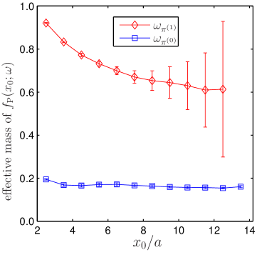
Figure 2: The effective mass in lattice units of the projected correlation functions $(\eta^{(0)},f_{\rm P})$ and $(\eta^{(1)},f_{\rm P})$ from run II.

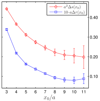
Figure 3: $\Delta s(x_{0})$ and $\Delta r(x_{0})$ determined from $\omega_{\pi^{(0)}}$ and $\omega_{\pi^{(1)}}$ in run II.

In Fig. 3 we show the effective masses from $f_{\rm P}(x_{0};\omega_{\pi^{(0)}})$ and $f_{\rm P}(x_{0};\omega_{\pi^{(1)}})$ as obtained in run II. Two distinct signals are clearly visible, which indicates that the described approximate projection method works well at these parameters. The energy of the first excited state is not far away from $a^{-1}$, suggesting that in even smaller volumes the residual $\textrm{O}(a^{2})$ effects would grow rapidly. In the spirit of the remark after eq. (18) at the other values of $\beta$ we used the same linear combination of wave functions to define $\omega_{\pi^{(0)}}$ and $\omega_{\pi^{(1)}}$, namely

$$\begin{array}[]{rcl}\eta^{(0)}&=&(\,0.5172,\,\phantom{-}0.6023,\,\phantom{-}0.6081\,)\\ \textrm{and}\quad\eta^{(1)}&=&(\,0.8545,\,-0.3233,\,-0.4066\,)\;,\end{array}$$ (20)

which are the ones determined in run II. When scaled in units of $r_{0}$, this yields effective masses similar to those shown in Fig. 3. Results from a redetermination of $\eta^{(0)}$ and $\eta^{(1)}$ in the other matched simulations would differ from eq. (20) only by $\sim 1\%$. In the figure the error on the effective mass of the first excited state is seen to be quite large, but what actually enters the computation of $c_{\rm A}$ is the error of

$$\Delta r(x_{0})=r(x_{0};\omega_{\pi^{(1)}})-r(x_{0};\omega_{\pi^{(0)}}) \Delta s(x_{0})=s(x_{0};\omega_{\pi^{(1)}})-s(x_{0};\omega_{\pi^{(0)}})\;.$$ and (21)

These profit from statistical correlations of the correlation functions entering their definition and thus have smaller statistical errors as can be seen in Fig. 3, where we plot $a\Delta r$ and $a^{2}\Delta s$ from the same data used in Fig. 3.

Fig. 4 collects results for the ”effective” $c_{\rm A}(x_{0})=-\Delta r(x_{0})/a\Delta s(x_{0})$ from the matched runs I-III. We see little variation for $x_{0}\gtrsim 6a$, which we take as another signal that high energy states which could contribute large $\textrm{O}(a)$ ambiguities in the improvement condition are reasonably suppressed in this region. We complete our definition of $c_{\rm A}$ with the choice $x_{0}\!=T/2$, which is at the same time scaled in physical units and in agreement with the $x_{0}\gtrsim 6a$ bound for all our lattices.

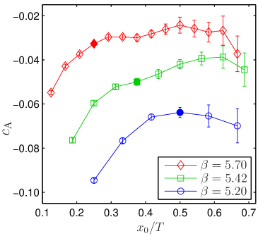
Figure 4: Effective $c_{\rm A}$ as determined from $\omega_{\pi^{(0)}}$ and $\omega_{\pi^{(1)}}$ for runs I-III. Points with $x_{0}/a=6$ are marked by filled symbols.

Finally, $c_{\rm A}$ is plotted as a function of $g_{0}^{2}$ in Fig. 5. The solid line is a smooth interpolation of the data from the matched simulations, constrained in addition by 1–loop perturbation theory:

$$c_{\rm A}(g_{0}^{2})=-0.00756\,g_{0}^{2}\times\frac{1-0.4485\,g_{0}^{2}}{1-0.8098\,g_{0}^{2}}.$$ (22)

It is our final result, valid in the range $0.98\leq g_{0}^{2}\leq 1.16$ within the errors of the data points (at most 0.004).

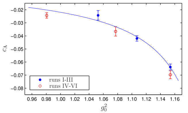
Figure 5: Simulation results for $c_{\rm A}$. The solid line represents a fit of the data points at constant physics (filled circles).

The non-perturbative result is quite far away form 1-loop perturbation theory, which takes a value of $c_{\rm A}=-0.0087$ at $g_{0}^{2}=1.15$. Using data from [36], we see that the effect on the result for the pseudo–scalar decay constant at this lattice spacing is as large as $10\%$.

3.2 Uncertainties due to deviations from the “constant physics” condition

We should check whether the volumes in our runs I-III are scaled sufficiently precisely or if systematic errors need to be added to the statistical ones on $c_{\rm A}$ to cover possible violations of the constant physics condition. Table 1 shows that the bare PCAC mass has been kept constant to within about 10%. A renormalized quark mass differs by the multiplication with a $Z$-factor which is a slowly varying function of $a$. As explained in the beginning of sect. 2, such a factor is irrelevant. Run IV is done with a quark mass which is more than a factor 2 larger than the one in run I, with otherwise identical parameters. The small difference in $c_{\rm A}$ confirms that the small deviations from the “constant mass” condition can be neglected.

The other issue is the uncertainty due to our perturbative (or asymptotic) scaling of the physical length scales. It has been argued in sect. 2.1 that the difference to a proper non-perturbative scaling is rather small. Also, estimating a possible change by comparing 3-loop to 2–loop and non–perturbative scaling, gives a deviation in $t(\beta)$ which is smaller than 10% in the whole range of Fig. 1 and thus the same maximum deviation applies to $L/a$. Again this can be neglected altogether. Additional confirmation comes from a comparison of the result from run V to our fit formula. In run V, $L/a$ is 20% lower than the proper value, but $c_{\rm A}$ does not differ significantly from the fit curve.

Finally, by run VI we verify that the dependence of $c_{\rm A}$ on the kinematic parameters disappears quickly when going to even larger values of $\beta$. In this run we used gauge configurations from the calculation of $Z_{\rm P}$ [37]. Although those were produced at $m\!=\!0$, $\theta\!=\!0.5$ and a much smaller volume, the resulting $c_{\rm A}$ is only approximately two standard deviations away from our fit.

4 Discussion

For the $\textrm{O}(a)$-improved action with non-perturbative $c_{\rm sw}$ [13], we have determined the improvement coefficient $c_{\rm A}$ for $\beta\!\geq\!5.2$, which roughly corresponds to $a\!\leq\!0.1$ fm. The improvement condition was implemented at constant physics, which is necessary in the situation when $\textrm{O}(a)$ ambiguities in the improvement coefficients are not negligible. This is indeed the case here: at $\beta\!=\!5.42$ we have evaluated $c_{\rm A}$ also for an $L/a\!=\!12,T/a\!=\!16$ geometry. The value of $c_{\rm A}$ is about a (statistically significant) 30% larger in magnitude than for the constant physics condition $L/a\!=\!16\!=\!T/a$. Thus, imposing the constant physics condition is important in the present case.

In addition, in order to safely exclude large $\textrm{O}(a)$ ambiguities, improvement conditions should only involve states with energy $E\ll a^{-1}$. On this requirement we had to compromise more than we would have liked to do. Our maximum values for $Ea$ are about $0.7$. Although this could have been improved by going to somewhat larger values of $L$ (and $T$), this would have made the numerical computation much more expensive.

We finally note that large $\textrm{O}(a^{2})$ effects have been found in the $N_{\rm f}\!=\!2$, $\textrm{O}(a)$-improved theory [17] at $\beta\!=\!5.2$. These may well be related to the not so small $\textrm{O}(a)$ ambiguity in $c_{\rm A}$ that we just mentioned. This can only be investigated further by studying the scaling violations in quantities such as $F_{\pi}r_{0}$ after improvement. Of course also the renormalization constant $Z_{\rm A}$ has to be known to carry out such a study. We are presently computing $Z_{\rm A}$ following the strategies of [38, 39]. As an immediate application one can then $\textrm{O}(a)$–improve and renormalize the bare pseudoscalar decay constants computed in [40, 36, 19].

Clearly, the method employed in this paper may also be useful to compute $c_{\rm A}$ in the three flavor case, where $c_{\rm sw}$ is known non–perturbatively with plaquette and Iwasaki gauge actions [41, 14, 42].

- [1] K. Symanzik, Continuum limit and improved action in lattice theories. 1. Principles and theory, Nucl. Phys. B226 (1983) 187.
- [2] K. Symanzik, Continuum limit and improved action in lattice theories. 2. O() nonlinear sigma model in perturbation theory, Nucl. Phys. B226 (1983) 205.
- [3] K. G. Wilson, Confinement of quarks, Phys. Rev. D10 (1974) 2445–2459.
- [4] B. Sheikholeslami and R. Wohlert, Improved continuum limit lattice action for QCD with Wilson fermions, Nucl. Phys. B259 (1985) 572.
- [5] M. Lüscher, S. Sint, R. Sommer, and P. Weisz, Chiral symmetry and O(a) improvement in lattice QCD, Nucl. Phys. B478 (1996) 365–400, [hep-lat/9605038].
- [6] M. Lüscher and P. Weisz, O(a) improvement of the axial current in lattice QCD to one–loop order of perturbation theory, Nucl. Phys. B479 (1996) 429–458, [hep-lat/9606016].
- [7] M. Lüscher, S. Sint, R. Sommer, P. Weisz, and U. Wolff, Non–perturbative O(a) improvement of lattice QCD, Nucl. Phys. B491 (1997) 323–343, [hep-lat/9609035].
- [8] T. Bhattacharya, R. Gupta, W.-J. Lee, and S. R. Sharpe, O(a) improved renormalization constants, Phys. Rev. D63 (2001) 074505, [hep-lat/0009038].
- [9] UKQCD Collaboration, S. Collins, C. T. H. Davies, G. P. Lepage, and J. Shigemitsu, A non–perturbative determination of the O(a) improvement coefficient and the scaling of and , Phys. Rev. D67 (2003) 014504, [hep-lat/0110159].
- [10] ALPHA Collaboration, M. Guagnelli et al., Non–perturbative results for the coefficients and in improved lattice QCD, Nucl. Phys. B595 (2001) 44–62, [hep-lat/0009021].
- [11] R. Sommer, A new way to set the energy scale in lattice gauge theories and its applications to the static force and in Yang-Mills theory, Nucl. Phys. B411 (1994) 839–854, [hep-lat/9310022].
- [12] S. Dürr and M. Della Morte, Exploring two non–perturbative definitions of , Nucl. Phys. Proc. Suppl. 129 (2004) 417–419, [hep-lat/0309169].
- [13] ALPHA Collaboration, K. Jansen and R. Sommer, O(a) improvement of lattice QCD with two flavors of Wilson quarks, Nucl. Phys. B530 (1998) 185–203, [hep-lat/9803017].
- [14] JLQCD Collaboration, N. Yamada et al., Non-perturbative O(a)-improvement of Wilson quark action in three-flavor QCD with plaquette gauge action, hep-lat/0406028.
- [15] ALPHA Collaboration, S. Capitani, M. Lüscher, R. Sommer, and H. Wittig, Non–perturbative quark mass renormalization in quenched lattice QCD, Nucl. Phys. B544 (1999) 669–698, [hep-lat/9810063].
- [16] ALPHA Collaboration, J. Garden, J. Heitger, R. Sommer, and H. Wittig, Precision computation of the strange quark’s mass in quenched QCD, Nucl. Phys. B571 (2000) 237–256, [hep-lat/9906013].
- [17] ALPHA Collaboration, R. Sommer et al., Large cutoff effects of dynamical Wilson fermions, Nucl. Phys. Proc. Suppl. 129 (2004) 405–407, [hep-lat/0309171].
- [18] QCDSF Collaboration, M. Göckeler et al., Determination of light and strange quark masses from full lattice QCD, hep-ph/0409312.
- [19] JLQCD Collaboration, S. Aoki et al., Light hadron spectroscopy with two flavors of O(a)–improved dynamical quarks, Phys. Rev. D68 (2003) 054502, [hep-lat/0212039].
- [20] ALPHA Collaboration, M. Della Morte et al., Computation of the strong coupling in QCD with two dynamical flavours, hep-lat/0411025.
- [21] A. Bode and H. Panagopoulos, The three–loop beta–function of QCD with the clover action, Nucl. Phys. B625 (2002) 198–210, [hep-lat/0110211].
- [22] A. Hasenfratz and P. Hasenfratz, The connection between the lambda parameters of lattice and continuum QCD, Phys. Lett. B93 (1980) 165.
- [23] H. Kawai, R. Nakayama, and K. Seo, Comparison of the lattice lambda parameter with the continuum lambda parameter in massless QCD, Nucl. Phys. B189 (1981) 40.
- [24] P. Weisz, On the connection between the lambda parameters of Euclidean lattice and continuum QCD, Phys. Lett. B100 (1981) 331.
- [25] S. Sint and R. Sommer, The running coupling from the QCD Schrödinger functional: A one loop analysis, Nucl. Phys. B465 (1996) 71–98, [hep-lat/9508012].
- [26] M. Lüscher and P. Weisz, Computation of the relation between the bare lattice coupling and the MS coupling in SU(N) gauge theories to two loops, Nucl. Phys. B452 (1995) 234–260, [hep-lat/9505011].
- [27] B. Allés, A. Feo, and H. Panagopoulos, The three–loop beta function in SU(N) lattice gauge theories, Nucl. Phys. B491 (1997) 498–512, [hep-lat/9609025].
- [28] C. Christou, A. Feo, H. Panagopoulos, and E. Vicari, The three–loop beta–function of SU(N) lattice gauge theories with Wilson fermions, Nucl. Phys. B525 (1998) 387–400, [hep-lat/9801007].
- [29] M. Lüscher, R. Narayanan, P. Weisz, and U. Wolff, The Schrödinger functional: A renormalizable probe for non–abelian gauge theories, Nucl. Phys. B384 (1992) 168–228, [hep-lat/9207009].
- [30] S. Sint, On the Schrödinger functional in QCD, Nucl. Phys. B421 (1994) 135–158, [hep-lat/9312079].
- [31] ALPHA Collaboration, M. Guagnelli, J. Heitger, R. Sommer, and H. Wittig, Hadron masses and matrix elements from the QCD Schrödinger functional, Nucl. Phys. B560 (1999) 465–481, [hep-lat/9903040].
- [32] ALPHA Collaboration, A. Bode, P. Weisz, and U. Wolff, Two loop computation of the Schrödinger functional in lattice QCD, Nucl. Phys. B576 (2000) 517–539, [hep-lat/9911018].
- [33] S. Sint and P. Weisz, Further results on O(a) improved lattice QCD to one-loop order of perturbation theory, Nucl. Phys. B502 (1997) 251–268, [hep-lat/9704001].
- [34] M. Hasenbusch, Speeding up the Hybrid-Monte-Carlo algorithm for dynamical fermions, Phys. Lett. B519 (2001) 177–182, [hep-lat/0107019].
- [35] ALPHA Collaboration, M. Della Morte, R. Hoffmann, F. Knechtli, and U. Wolff, Impact of large cutoff–effects on algorithms for improved Wilson fermions, Comput. Phys. Commun. 165 (2005) 49–58, [hep-lat/0405017].
- [36] UKQCD Collaboration, A. C. Irving, C. McNeile, C. Michael, K. J. Sharkey, and H. Wittig, Is the up-quark massless?, Phys. Lett. B518 (2001) 243–251, [hep-lat/0107023].
- [37] ALPHA Collaboration, M. Della Morte et al., Simulating the Schrödinger functional with two pseudo–fermions, Comput. Phys. Commun. 156 (2003) 62–72, [hep-lat/0307008].
- [38] M. Lüscher, S. Sint, R. Sommer, and H. Wittig, Non–perturbative determination of the axial current normalization constant in O(a) improved lattice QCD, Nucl. Phys. B491 (1997) 344–364, [hep-lat/9611015].
- [39] R. Hoffmann, F. Knechtli, J. Rolf, R. Sommer, and U. Wolff, Non–perturbative renormalization of the axial current with improved Wilson quarks, Nucl. Phys. Proc. Suppl. 129 (2004) 423–425, [hep-lat/0309071].
- [40] UKQCD Collaboration, C. R. Allton et al., Effects of non–perturbatively improved dynamical fermions in QCD at fixed lattice spacing, Phys. Rev. D65 (2002) 054502, [hep-lat/0107021].
- [41] CP-PACS Collaboration, S. Aoki et al., Non–perturbative determination of in three–flavor dynamical QCD, Nucl. Phys. Proc. Suppl. 119 (2003) 433–435, [hep-lat/0211034].
- [42] CP-PACS Collaboration, K. I. Ishikawa et al., Study of finite volume effects in the non–perturbative determination of with the SF method in full three–flavor lattice QCD, Nucl. Phys. Proc. Suppl. 129 (2004) 444–446, [hep-lat/0309141].