Abstract

We present a Lattice QCD determination of the chiral quark condensate based on a new method. We extract the quark condensate from the operator product expansion of the quark propagator at short euclidean distances, where it represents the leading contribution in the chiral limit. From this study we obtain $\langle\bar{q}q\rangle^{{\overline{\rm{MS}}}}(2\,\textrm{GeV})=-(265\pm 5\pm 22~{}\textrm{MeV})^{3}$, in good agreement with determinations of this quantity based on different approaches. The simulation is performed by using the ${\cal O}(a)$-improved Wilson action at $\beta=6.45$ on a volume $32^{3}\times 70$ in the quenched approximation.

1 Introduction

An accurate determination of the chiral quark condensate is a task of prime interest. Its non-vanishing value signals the spontaneous breaking of chiral symmetry in QCD and, quantitatively, it is related to the pseudo-Goldstone bosons mass spectrum.

Due to the purely non-perturbative nature of the quark condensate, its estimate is rather challenging. Traditional approaches have been based on QCD sum rules (a review of these techniques can be found in refs. [1, 2]). In the last years, first principle determinations of the quark condensate have been provided by Lattice QCD calculations, and the accuracy of these results is expected to systematically improve in time. The standard method to extract the quark condensate from lattice calculations exploits the well known GMOR formula [3]-[6]. Alternative techniques have been also investigated, based on the $\epsilon$-expansion of QCD in a small volume [7]-[9] and on the study of the Goldstone pole contribution to the pseudoscalar quark Green function [10, 11].

In this paper, we present an exploratory Lattice QCD determination of the chiral quark condensate based on a new method. We study the quark propagator in coordinate space and its operator product expansion (OPE) [12] at short euclidean distances. The OPE is a powerful technique that systematically includes non-perturbative corrections and parameterizes the non-trivial properties of the QCD vacuum in terms of condensates [13]. We extract the quark condensate $\langle\bar{\psi}\psi\rangle$ by evaluating the quark propagator at short distances on the lattice, and comparing the result with the OPE prediction,

$$S(x)\;\sim\;C_{I}(x)\,\frac{\hbox to0.0pt{\hbox to5.71527pt{\hfil/\hfil}\hss}x}{(x^{2})^{2}}\;+\;C_{m}(x)\,\frac{m}{x^{2}}\;+\;C_{\bar{\psi}\psi}(x)\,\langle\bar{\psi}\psi\rangle\;+\;\ldots$$ (1)

where the dots represent higher powers of $x^{2}$ and of the quark mass $m$. Our final result for the chiral quark condensate, renormalized in the ${\overline{\rm{MS}}}$ scheme at the scale $\mu=2$ GeV, is

$$\langle\bar{q}q\rangle^{{\overline{\rm{MS}}}}(2\,\textrm{GeV})=-(265\pm 5\pm 22~{}\textrm{MeV})^{3}\,,$$ (2)

where the first error is statistical and the second systematic. This result is in good agreement with those obtained from the other methods listed above. It also provides a remarkable non-perturbative test of the OPE predictions at short distance in QCD.

The OPE of the quark propagator can be also performed in momentum space, from which a determination of the quark condensate might be possible as well. When working on the lattice with Wilson fermions, however, the leading contribution to the OPE in momentum space is a constant term induced by discretization effects. Though vanishing in the continuum limit, this term is dominant at fixed lattice spacing with respect to the mass and the condensate contributions, whose coefficients are suppressed by $1/p^{2}$ and $1/p^{4}$ respectively [14]. In coordinate space this major obstacle is bypassed, since the Fourier transform of the unphysical term is a discretized delta function, whose effect is negligible at distances larger than few lattice spacings.

Another advantage of the approach studied in this paper is that it greatly simplifies the renormalization procedure. Specifically, once the quark propagator on the l.h.s. of eq. (1) is renormalized, all contributions appearing on the r.h.s. turn out to be expressed in terms of renormalized quantities. In particular, the determination of the chiral quark condensate in this approach does not require the evaluation of the corresponding renormalization constant.

The applicability of the OPE to correlation functions evaluated on the lattice at fixed value of the lattice spacing $a$ relies on the existence of a short distance region where the conditions

$$a\mathrel{\hbox to0.0pt{\raise 2.20013pt\hbox{$<$}\hss}{\lower 2.20013pt\hbox{$\sim$}}}x\mathrel{\hbox to0.0pt{\raise 2.20013pt\hbox{$<$}\hss}{\lower 2.20013pt\hbox{$\sim$}}}1/\Lambda_{\rm QCD}$$ (3)

are both satisfied. The upper bound in eq. (3) guarantees that the Wilson coefficients entering the OPE at the typical scale $\mu=1/x$ can be evaluated in perturbation theory. The lower bound must be satisfied in order to keep under control discretization effects. In the present study, though we use an ${\cal O}(a)$-improved action and the value of the inverse lattice spacing is as large as $a^{-1}\simeq$ 4 GeV, we find that in the region $x\mathrel{\hbox to0.0pt{\raise 2.20013pt\hbox{$<$}\hss}{\lower 2.20013pt\hbox{$\sim$}}}1/\Lambda_{\rm QCD}$ discretization effects in the quark propagator are not negligible. These effects are in fact responsible for most of the systematic uncertainty quoted in eq. (2). In order to reduce their contribution, we have followed a procedure similar to the one applied in ref. [15]: we have corrected the lattice results for the quark propagator by the lattice artifacts computed in the free theory, thus reducing their size from ${\cal O}(a^{2})$ to ${\cal O}(\alpha_{s}\,a^{2})$.

We now summarize the procedure followed in this study and present the plan of the paper.

– In sect.2, we derive the OPE of the quark propagator in coordinate space, by including QCD corrections up to the next-to-leading order (NLO).

– Details of the lattice simulation are presented in sect.3, where the tree-level correction of lattice artifacts is also discussed.

– In sect.4 we compute the renormalization constant of the quark propagator non-perturbatively in the $X$-space scheme. The $X$-space method has been proposed in ref. [16], and applied in [15] to compute the renormalization constants of bilinear quark operators. Our result for the quark field renormalization constant, converted to the ${\overline{\rm{MS}}}$ scheme, reads

$$Z_{\psi}^{{\overline{\rm{MS}}}}(\mu=2\ {\rm GeV})=0.871\pm 0.003\pm 0.020\,,$$ (4)

in good agreement with the result obtained in ref. [17] by using the non-perturbative RI-MOM method.

– In sect.5 we evaluate the chiral quark condensate by fitting in coordinate space the quark propagator, extrapolated to the chiral limit, to its OPE. A second estimate is obtained by first using the OPE at finite values of the quark mass and then extrapolating the result to the chiral limit. Different functional forms are considered in the fits, and the differences among the results are taken into account in the estimate of the systematic error. The two approaches give completely consistent results.

– The final result quoted in eq. (2) is presented in sect.6, where we discuss in details the evaluation of the systematic error.

– Finally, we sketch in the appendix the NLO QCD calculation of the Wilson coefficients entering in eq. (1)

2 OPE of the quark propagator in coordinate space

The quark propagator can be expressed in terms of two scalar form factors, $\Sigma_{1}(x)$ and $\Sigma_{2}(x)$, which are defined from

$$S(x)=\frac{\hbox to0.0pt{\hbox to5.71527pt{\hfil/\hfil}\hss}x}{(x^{2})^{2}}\,\Sigma_{1}(x)+\frac{1}{x^{2}}\,\Sigma_{2}(x).$$ (5)

The leading terms in the OPE of $\Sigma_{1}(x)$ and $\Sigma_{2}(x)$ can be read from eq. (1):

$$\Sigma_{1}(x) = \frac{1}{2\pi^{2}}\,C_{I}(x)+\cdots$$

$$\Sigma_{2}(x) = \frac{1}{4\pi^{2}}\,C_{m}(x)\,m-\frac{1}{4N_{c}}\,C_{\bar{\psi}\psi}(x)\,\langle\bar{\psi}\psi\rangle\,x^{2}+\cdots$$ (6)

where, at variance with eq. (1), the Wilson coefficients $C_{I}(x),\,C_{m}(x)$ and $C_{\bar{\psi}\psi}(x)$ are normalized to unity in the free theory. $N_{c}$ is the number of colors and the quark condensate is defined as

$$\langle\bar{\psi}\psi\rangle\equiv\langle\bar{\psi}_{i}^{\alpha}(0)\psi_{i}^{\alpha}(0)\rangle\,,$$ (7)

where a summation over repeated color and spin indices is understood.

By using the known two-loop results for the quark field and the quark mass anomalous dimensions in QCD, a simple one-loop calculation provides the renormalization group improved expressions for the Wilson coefficients in eq. (6), at the NLO. The main steps of the calculation are given in the appendix. We find, in the ${\overline{\rm{MS}}}$ scheme,

$$\Sigma^{{\overline{\rm{MS}}}}_{1}(x,\mu)={\displaystyle{1\over 2\pi^{2}}}\,W_{\psi}(\mu,1/x)\left[1-2{\displaystyle{\alpha_{s}(1/x)\over 4\pi}}C_{F}\xi\left(\gamma_{E}-\log 2\right)\right]$$ (8)

$$\Sigma^{{\overline{\rm{MS}}}}_{2}(x,\mu) = W_{\psi}(\mu,1/x)\left[1-2{\displaystyle{\alpha_{s}(1/x)\over 4\pi}}C_{F}\xi\left(\gamma_{E}-\log 2\right)\right]$$

$$\left\{{\displaystyle{1\over 4\pi^{2}}}W_{m}(\mu,1/x)\left[1+{\displaystyle{\alpha_{s}(1/x)\over 4\pi}}C_{F}\left(4-2(\xi-3)(\gamma_{E}-\log 2)\right)\right]m^{\overline{\rm{MS}}}(\mu)\right.$$

$$\left.-{\displaystyle{1\over 4N_{c}}}W^{-1}_{m}(\mu,1/x)\left[1+2{\displaystyle{\alpha_{s}(1/x)\over 4\pi}}C_{F}\left(1-(\xi+3)(\gamma_{E}-\log 2)\right)\right]\langle\bar{\psi}\psi\rangle^{\overline{\rm{MS}}}(\mu)\,x^{2}\right\}\,.$$

The terms in square brackets represent the Wilson coefficients at the scale $\mu=1/x$, whereas $W_{I}(\mu,1/x)$, with $I=\psi,m$, are the NLO evolution functions,

$$W_{I}(\mu,1/x)=\left({\displaystyle{\alpha_{s}(1/x)\over\alpha_{s}(\mu)}}\right)^{\frac{\gamma^{0}_{I}}{2\beta_{0}}}\left[1+\left({\displaystyle{\beta_{1}\gamma^{0}_{I}\over 2\beta_{0}^{2}}}-{\displaystyle{\gamma^{1}_{I}\over 2\beta_{0}}}\right){\displaystyle{\alpha_{s}(\mu)-\alpha_{s}(1/x)\over 4\pi}}\right]\,.$$ (10)

The coefficients of the beta function and of the quark mass and quark field anomalous dimensions at the LO and NLO read:

$$\beta_{0} = {\displaystyle{11N_{c}-2n_{f}\over 3}}\quad,\quad\beta_{1}={\displaystyle{34\over 3}}N_{c}^{2}-{\displaystyle{10\over 3}}N_{c}n_{f}-2C_{F}n_{f}$$

$$\gamma^{0}_{m} = 6\,C_{F}\quad,\quad\gamma^{1}_{m}=C_{F}\left(\frac{97}{3}N_{c}+3C_{F}-{\displaystyle{10\over 3}}n_{f}\right)$$ (11)

$$\gamma^{0}_{\psi} = -2\xi C_{F}\quad,\quad\gamma^{1}_{\psi}=-4\,C_{F}\left(\left({\displaystyle{25\over 8}}+\xi+{\displaystyle{\xi^{2}\over 8}}\right)N_{c}-{\displaystyle{1\over 2}}n_{f}-{\displaystyle{3\over 4}}C_{F}\right)$$

where $C_{F}=(N^{2}_{c}-1)/(2N_{c})$, $\xi$ is the gauge parameter ($\xi=0$ in the Landau gauge) and $n_{f}$ is the number of active flavors ($n_{f}=0$ in the quenched approximation).

The result in coordinate space for the Wilson coefficient of the quark condensate given in eq. (2) corresponds to the one obtained in ref. [18] in momentum space. Eqs. (8) and (2) will be used in sects.4 and 5 to extract the quark field renormalization constant and the chiral quark condensate with NLO accuracy in the ${\overline{\rm{MS}}}$ scheme.

3 Analysis of discretization effects

In this section we present the details of the lattice simulation, illustrate the results obtained for the bare quark propagator and discuss the free theory correction implemented in order to reduce the lattice artifacts.

We have generated $180$ gauge configurations in the quenched approximation with the non-perturbatively ${\cal O}(a)$-improved Wilson action on a volume $32^{3}\times 70$ at $\beta=6.45$. As a value of the inverse lattice spacing we use $a^{-1}=3.87(19)\ {\rm GeV}$, as obtained in ref. [19] from the studies of the quark-antiquark potential [20] and by using in input the reference scale $a^{-1}(\beta=6.0)=2.0(1)\ {\rm GeV}$. We have computed the quark propagator at four values of the hopping parameter, $\kappa=$ 0.1349, 0.1351, 0.1352, 0.1353, corresponding to light quark masses in the range $m_{s}/2\mathrel{\hbox to0.0pt{\raise 2.20013pt\hbox{$<$}\hss}{\lower 2.20013pt\hbox{$\sim$}}}m\mathrel{\hbox to0.0pt{\raise 2.20013pt\hbox{$<$}\hss}{\lower 2.20013pt\hbox{$\sim$}}}m_{s}$. The corresponding values of the renormalized quark masses have been obtained in ref. [19] from the study of both the vector and axial-vector Ward identities, and are given in lattice units, in the ${\overline{\rm{MS}}}$ scheme, in table 1. These values have been used in the study of the OPE of the quark propagator and to perform the chiral extrapolations of the quantities we are interested in. The statistical errors quoted in this paper have been evaluated with the jackknife technique.

$\kappa$	0.1349	0.1351	0.1352	0.1353
$am^{{\overline{\rm{MS}}}}_{AWI}(2\ {\rm GeV})$	0.0305(4)	0.0227(3)	0.0188(2)	0.0149(2)
$am^{{\overline{\rm{MS}}}}_{VWI}(2\ {\rm GeV})$	0.0288(3)	0.0215(2)	0.0178(2)	0.0141(1)

Table 1: Quark masses in lattice units for the non-perturbatively ${\cal O}(a)$-improved Wilson action at $\beta=6.45$. The results are taken from ref. [19] (where they are quoted in the RI-MOM scheme at the scale $\mu=3\ {\rm GeV}$).

We have fixed the Landau gauge on the lattice by minimizing the quantity:

$$\theta=\frac{1}{V}\,\sum_{x}\,{\rm Tr}\,\left[\,\Delta_{\mu}A_{\mu}(x)\,\Delta_{\nu}A_{\nu}(x)\,\right]$$ (12)

where $V$ is the lattice volume and $\Delta_{\mu}A_{\mu}$ is the discretized version of the gauge field divergence $\partial_{\mu}\,A_{\mu}$. We have required $\theta\leq 5.0\times 10^{-4}$ for all the configurations used in this study.

In order to compute the quark condensate and the quark field renormalization constant, we have extracted from the quark propagator in the Landau gauge the bare form factors $\Sigma_{1}(x)$ and $\Sigma_{2}(x)$ defined in eq. (5). The results are shown in fig. 1(top) for $\kappa=0.1349$ as functions of $(x/a)^{2}$.

Figure 1: The bare form factors $\Sigma_{1}$ (left panels) and $\Sigma_{2}$ (right panels). We show, from top to bottom: the form factors in the interacting theory, as obtained from the lattice simulation at k=0.1349; the form factors computed in the free lattice theory, at infinite volume and in the chiral limit; the “corrected” form factors defined in eqs. (13) and (14).

Lorentz invariance requires that, when approaching the continuum limit, the form factors should become functions of $x^{2}$ only. At fixed value of the lattice spacing, however, the plots in fig. 1(top) show that points corresponding to the same value of $(x/a)^{2}$ are significantly spreaded out. This is true especially at short distances ($(x/a)^{2}\mathrel{\hbox to0.0pt{\raise 2.20013pt\hbox{$<$}\hss}{\lower 2.20013pt\hbox{$\sim$}}}10$), where discretization effects are expected to be larger. A better understanding of these effects can be obtained by studying the lattice quark propagator in the free theory. Indeed, in the short distance region which is relevant for the $X$-space method the interacting theory is expected to approach the asymptotic free regime, up to small perturbative corrections. One finds that $\Sigma_{1}(x)$ and $\Sigma_{2}(x)$, computed on the lattice in the free theory, present similar deviations from the expected continuum behavior. The free theory results, obtained at infinite volume and in the chiral limit, are shown in fig. 1(center), and they can be compared with the lattice results shown in the top panels. This similarity suggests that one can identify the discretization patterns in the free case in order to subtract them in the interacting case of interest [15]. The practical implementation of this approach passes through the definition of the “corrected” form factors.

In the case of $\Sigma_{1}(x)$ we define

$$\Sigma_{1}^{corr}(x)=\left(\frac{\Sigma^{cont}_{1,\,free}(x)}{\Sigma^{lat}_{1,\,free}(x)}\right)\,\Sigma_{1}(x)\,,$$ (13)

where $\Sigma^{cont}_{1,\,free}(x)$ and $\Sigma^{lat}_{1,\,free}(x)$ are the free theory form factors computed respectively in the continuum and on the lattice, at infinite volume and in the chiral limit. For finite values of the lattice spacing, the difference of the ratio $\Sigma^{cont}_{1,\,free}(x)/\Sigma^{lat}_{1,\,free}(x)$ from unity is a measure of tree-level discretization errors. After the correction of eq. (13), we expect these errors to be reduced from $O(a^{2})$ to $O(\alpha_{s}a^{2})$.

Concerning $\Sigma_{2}(x)$ one observes that, in the continuum and in the chiral limit, the form factor vanishes at any order of perturbation theory. Therefore, in the case of $\Sigma_{2}$ we implement the following correction:

$$\Sigma_{2}^{corr}(x)=\Sigma_{2}(x)-\Sigma^{lat}_{2,\,free}(x),$$ (14)

where $\Sigma^{lat}_{2,\,free}$ represents a pure discretization effect. After eqs. (13) and (14) have been implemented, we also average the results for the form factors $\Sigma_{1}(x)$ and $\Sigma_{2}(x)$ obtained at lattice points which correspond to the same value of $x^{2}$.

The remarkable effect of the correction on the two form factors is shown in fig. 1 (bottom). In the following analysis, otherwise indicated, we will always use the corrected form factors defined in eqs. (13) and (14).

4 Renormalization of the quark propagator in the X-scheme

In this section, we define the $X$-space renormalization scheme [15] for the quark propagator and discuss the determination of the corresponding renormalization constant.

The quark field renormalization constant $Z_{\psi}^{X}(\mu)$, in the Landau gauge $X$-scheme, is determined non-perturbatively by imposing the condition

$$Z_{\psi}^{X}(\mu=1/x)\,\Sigma_{1}(x)\left|{}^{\xi=0}_{m\to 0}\right.=\Sigma^{cont}_{1,\,free}(x)$$ (15)

where the value of the form factor in the free continuum theory and in the chiral limit is $\Sigma^{cont}_{1,\,free}(x)=1/(2\pi^{2})$. The limit $m\to 0$ in eq. (15) guarantees a mass-independent definition of the renormalization scheme. It also guarantees that, when using the ${\cal O}(a)$-improved Wilson action, the renormalization constant computed from eq. (15) is automatically ${\cal O}(a)$-improved, without need of further improving the quark field [17].

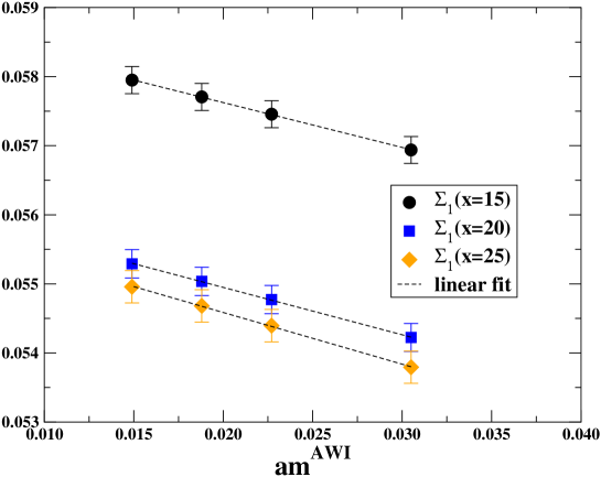
In order to extrapolate the form factor $\Sigma_{1}(x)$ to the chiral limit we have assumed a linear dependence on the quark mass. This dependence describes well the lattice data as can be seen from fig. 2, where the linear fit is shown for three values of $x^{2}$ in the range of interest. A quadratic fit has been also performed in order to evaluate the systematic error involved in the chiral extrapolation.

Figure 2: Quark mass dependence of $\Sigma_{1}(x)$ at three different values of $x^{2}$. The dashed lines represent the result of a linear fit.

By combining the renormalization condition (15) with the NLO evolution function of $Z_{\psi}$ given in eq. (10) and considering that the LO anomalous dimension of the quark field vanishes in the Landau gauge, one finds at the NLO

$$Z_{\psi}^{X}(\mu)=W_{\psi}(\mu,1/x)\,Z_{\psi}^{X}(1/x)=\left(1-{\displaystyle{\gamma^{1}_{\psi}\over 2\beta_{0}}}{\displaystyle{\alpha_{s}(\mu)-\alpha_{s}(1/x)\over 4\pi}}\right)\left(\frac{\Sigma^{cont}_{1,\,free}(x)}{\Sigma_{1}(x)}\right)\,.$$ (16)

We also note that, in the Landau gauge, the equality of the renormalized form factor $\Sigma_{1}(x)$ at one loop in the ${\overline{\rm{MS}}}$ and $X$ schemes implies that the NLO anomalous dimensions $\gamma^{1}_{\psi}$ are also equal in the two schemes. In the numerical analysis, $\alpha_{s}(1/x)$ has been evaluated at the NLO in the ${\overline{\rm{MS}}}$ scheme by using $n_{f}=0$ and the quenched estimate $\Lambda_{QCD}^{n_{f}=0}=0.225(21)\ {\rm GeV}$ (obtained from $r_{0}\Lambda_{QCD}^{n_{f}=0}=0.602(48)$ [21] and using $r_{0}=0.525(25)$ fm).

As already discussed in the introduction, the $X$-space non-perturbative renormalization approach relies on the existence of a window $a\mathrel{\hbox to0.0pt{\raise 2.20013pt\hbox{$<$}\hss}{\lower 2.20013pt\hbox{$\sim$}}}x\mathrel{\hbox to0.0pt{\raise 2.20013pt\hbox{$<$}\hss}{\lower 2.20013pt\hbox{$\sim$}}}1/\Lambda_{\rm QCD}$ which permits matching the lattice results with the perturbative ones and, at the same time, to avoid the region at very short distances affected by contact terms and large discretization effects. In practice, in the present study, we consider this condition satisfied in the range $9\mathrel{\hbox to0.0pt{\raise 2.20013pt\hbox{$<$}\hss}{\lower 2.20013pt\hbox{$\sim$}}}(x/a)^{2}\mathrel{\hbox to0.0pt{\raise 2.20013pt\hbox{$<$}\hss}{\lower 2.20013pt\hbox{$\sim$}}}25$ (the upper bound corresponds to $x^{-1}\sim 1\ {\rm GeV}$).

The results for $Z_{\psi}^{X}(\mu=2\ {\rm GeV})$ as obtained from eq. (16) at different values of $x^{2}$ are shown in fig. 3. One observes that even in the region $(x/a)^{2}=[9,25]$ the data show some spread, at the level of few percent. This spread is due to discretization errors which remain after the free theory correction has been implemented. It represents the main source of systematic uncertainty in the evaluation of $Z_{\psi}$.

Figure 3: Values of $Z_{\psi}^{X}(\mu=2\ {\rm GeV})$ as obtained from eq. (16) for different values of $(x/a)^{2}$. The solid lines indicate the results obtained from a constant fit in $x^{2}$ and the estimated systematic error (eq. (17)). The dashed vertical lines show the range in $(x/a)^{2}$ where the constant fit is performed. The result of a linear fit in $x^{2}$ is also shown (dashed line). In the latter case, the estimate of $Z_{\psi}^{X}(\mu=2\ {\rm GeV})$ is given by the intercept.

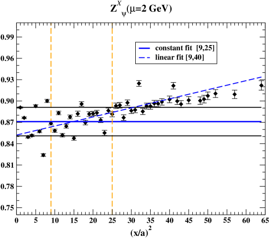
A second source of uncertainty is due the fact that one cannot exclude, even in the fitting region $(x/a)^{2}=[9,25]$, a systematic dependence of the data on $x^{2}$, which could be due to higher order contributions to the OPE of $\Sigma_{1}(x)$ neglected in eq. (6). In order to evaluate this systematics, we have evaluated $Z_{\psi}(\mu)$ from both a constant and linear fit in $(x/a)^{2}$, by considering in the latter case larger intervals in $x^{2}$ (up to $(x/a)^{2}=40$). The results of the fits are presented in table 2.

$Z_{\psi}^{X}(\mu)$	$(x/a)^{2}$-range	fit
$0.871\pm 0.003$	$[9,25]$	constant
$0.852\pm 0.003$	$[9,40]$	linear

Table 2: $Z_{\psi}(\mu)$ in the $X$-space scheme at $\mu=2\ {\rm GeV}$ as obtained from either a constant or a linear fit in $x^{2}$. The quoted errors are statistical only.

The other sources of systematic effects, as those deriving from the determination of the lattice scale, the estimate of $\Lambda_{\rm QCD}$, the difference between linear and quadratic chiral extrapolations and the use of the vector or the axial-vector definitions of the quark masses in these extrapolations, are found to be negligible. As final estimate of $Z_{\psi}^{X}(\mu)$ we thus quote

$$Z_{\psi}^{X}(2\ {\rm GeV})=0.871\pm 0.003\pm 0.020$$ (17)

where the first error is statistical and the second systematic. The central value in eq. (17) is the one obtained from the constant fit in the shorter distance range $(x/a)^{2}=[9,\,25]$, where the contribution of higher power corrections is more suppressed. The few percent error on the value of $Z_{\psi}$ introduces an uncertainty in the estimate of the chiral quark condensate discussed in the next section which is completely negligible.

The vanishing of the one-loop contribution to the form factor $\Sigma_{1}(x)$ in the Landau gauge implies that the quark field renormalization constant at the NLO is equal in several commonly used renormalization schemes. In particular,

$$Z_{\psi}^{X}(\mu)=Z_{\psi}^{{\overline{\rm{MS}}}}(\mu)=Z_{\psi}^{\rm{RI-MOM}}(\mu)$$ (18)

at the NLO. The result in eq. (17) can be therefore directly compared to the value $Z_{\psi}^{\rm{RI-MOM}}(2\ {\rm GeV})=0.865\pm 0.003$ obtained non-perturbatively in ref. [17] by using the RI-MOM method. It can be also compared with the prediction of one-loop boosted perturbation theory $Z_{\psi}^{{\overline{\rm{MS}}}}(2\ {\rm GeV})\simeq 0.880$.

We also quote the value of $Z_{\psi}^{X}$ obtained by using the rough lattice data, without implementing the tree-level correction of discretization effects: $Z^{X}_{\psi}(2\ {\rm GeV})=0.868\pm 0.003\pm 0.080$. The difference in the central value with respect to eq. (17) is less than 0.5%. As expected, however, the systematic uncertainty is much larger in the latter case, due to the significantly larger spread of the points in the fitting region. In practice, the tree-level correction has smoothed the overall behavior of the quark propagator at short distances allowing the reduction of the systematic uncertainty by about a factor $4$, but affecting the central value by only a small amount.

5 Extraction of the quark condensate

One of the advantages of the approach considered in this paper to evaluate the chiral quark condensate is that the renormalization procedure is greatly simplified: in the OPE of the quark propagator, expressed by eq. (1), once the propagator on the l.h.s. is renormalized by the quark field renormalization constant, the r.h.s. turns out to be expressed directly in terms of renormalized quantities. In particular, the quark condensate, renormalized at a scale $\mu$, can be extracted directly from the trace of the quark propagator (i.e. the scalar form factor $\Sigma_{2}$) renormalized at the same scale. Furthermore, once the quark propagator is improved at ${\cal O}(a)$, the operator matrix elements which enter its OPE are automatically improved at the same order.

In the study of the OPE, the physical quantity which we are interested in is the quark condensate in the chiral limit. To reach this limit, we have followed two procedures. In the first approach, we extrapolate to the chiral limit the scalar form factor $\Sigma_{2}(x)$ for each value of $x^{2}$. The quark condensate is then evaluated by using the OPE expressed by eq. (2), which is accurate at the NLO, in the massless case. In this limit, the quark condensate represents the leading term of the expansion. In the second approach, which we consider for a consistency check of the calculation, the order of the extrapolations is inverted. At finite values of the quark mass, the OPE of $\Sigma_{2}$ at order $x^{2}$ contains, besides the quark condensate, a term proportional to $m^{3}$. In this case, we first extract the whole ${\cal O}(x^{2})$ contribution to the OPE and then extrapolate the result to the chiral limit. As we will show in the following, the two procedures yield completely consistent predictions. We now discuss the two approaches in more detail.

Method I:

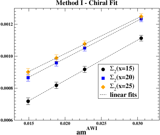
For each value of $x^{2}$, the renormalized form factor $\Sigma_{2}(x)$ is extrapolated to the chiral limit, both linearly and quadratically in either the vector or the axial-vector quark masses. Examples of this chiral extrapolation, for three typical values of $x^{2}$, are shown in fig. 4. For each value of $x^{2}$ we have then computed the quantity

$$Q_{I}(x,\mu)\equiv-\frac{(\Sigma_{2}^{{\overline{\rm{MS}}}}(x,\mu))^{\rm chiral}}{C_{\bar{\psi}\psi}(x,\mu)\,x^{2}/4N_{c}}=\langle\bar{\psi}\psi\rangle^{\overline{\rm{MS}}}(\mu)+{\cal O}(x^{2})$$ (19)

and performed a fit to the form

$$Q_{I}(x,\mu)=\langle\bar{\psi}\psi\rangle^{\overline{\rm{MS}}}(\mu)+B\,x^{2}\,.$$ (20)

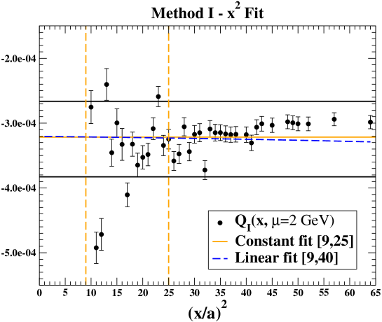
Both constant ($B=0$) and linear fits have been performed, and the results are presented in table 3, see also fig. 5. Since the results of the linear fit are unstable when the fit is limited to the interval $(x/a)^{2}=[9,\,25]$, we have considered in this case larger distances, up to $(x/a)^{2}=40$. In all cases, we find consistent results for the quark condensate, as can be seen from table 3. We also find that the contribution of the ${\cal O}(x^{2})$ term is completely negligible, and the coefficient B is compatible with zero within the statistical errors.

$\langle\bar{\psi}\psi\rangle^{{\overline{\rm{MS}}}}(\mu=2\ {\rm GeV})[\ {\rm MeV}^{\,3}]$		$(x/a)^{2}$-range
Constant fit	Linear fit
$-(265\pm 5)^{3}$	$-$	$[9,25]$
$-(266\pm 4)^{3}$	$-(265\pm 7)^{3}$	$[9,40]$

Table 3: Values of the chiral quark condensate in the ${\overline{\rm{MS}}}$ scheme at the scale $\mu=2\ {\rm GeV}$ as obtained from either the constant or the linear fit of eq. (20).

Figure 4: Quark mass dependence of $\Sigma_{2}(x)$ at three different values of $x^{2}$. The dashed lines represent the result of a linear fit.

Figure 5: Values of $Q_{I}(x,\mu=2\ {\rm GeV})$ as a function of $(x/a)^{2}$. The solid lines indicate the results obtained from a constant fit in $x^{2}$ and the estimated systematic error. The dashed vertical lines show the range in $(x/a)^{2}$ where the constant fit is performed. The result of the linear fit in $x^{2}$ is also shown (dashed line).

As a further check of our results, we have also extracted the quark condensate directly from the ratio $\Sigma_{2}/\Sigma_{1}$ of the two form factors. From eq. (6) one finds that, in the chiral limit, this ratio behaves as

$$\frac{\Sigma_{2}^{X}(x,\mu)}{\Sigma_{1}^{X}(x,\mu)}=\frac{\Sigma_{2}(x)}{\Sigma_{1}(x)}=-\frac{\pi^{2}}{2N_{c}}\frac{C_{\bar{\psi}\psi}(x,\mu)}{C_{I}(x,\mu)}\,\langle\bar{\psi}\psi\rangle^{\overline{\rm{MS}}}(\mu)+{\cal O}(x^{2})\,.$$ (21)

The determination of the quark condensate from eq. (21) bypasses the evaluation of the quark field renormalization constant $Z_{\psi}$. This constant cancels in the ratio, since it enters the renormalization of both the form factors $\Sigma_{1}$ and $\Sigma_{2}$. This also implies that the r.h.s. of eq. (21) is independent of the choice of the renormalization scale $\mu$. We also find that this ratio, when computed by using the non-corrected form factors, exhibits a more stable plateau as a function of $x^{2}$. The results for the quark condensate obtained with the two approaches are in excellent agreement (within less than 2%), indicating that the uncertainty connected with the evaluation of $Z_{\psi}$ is actually negligible.

Method II:

In this second approach we study the OPE of $\Sigma_{2}(x)$ at finite values of the quark mass, extract the ${\cal O}(x^{2})$ contribution to the expansion and extrapolate it to the chiral limit, in order to get the chiral quark condensate.

The fit of the form factor $\Sigma_{2}$ to its OPE is shown in fig. 6, for two values of the quark mass.

Figure 6: Values of $\Sigma_{2}^{X}(x,\mu=2\ {\rm GeV})$ as a function of $(x/a)^{2}$ for two different values of the quark mass. The solid lines represent the results of the fit to the OPE prediction performed by using for the renormalized quark masses the values given in table 1.

Figure 7: Linear fit of $Q_{II}(m,\mu=2\ {\rm GeV})$ as a function of the quark mass. The extrapolated value is the chiral quark condensate in lattice units.

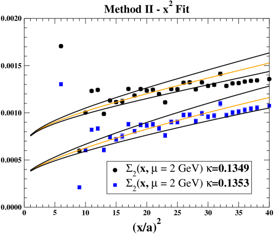
We find that the mass term contribution to the OPE, which is leading at very short distances where lattice artifacts are more severe, is poorly estimated from the fit. For this reason, we have chosen to fix the renormalized quark mass in eq. (2) to the values determined in ref. [19] and collected in table 1. Therefore, for each value of the quark mass we compute the quantity

$$Q_{II}(x,m,\mu)\equiv-\frac{\Sigma_{2}^{{\overline{\rm{MS}}}}(x,\mu)-C_{m}(x,\mu)\,m^{\overline{\rm{MS}}}(\mu)/4\pi^{2}}{C_{\bar{\psi}\psi}(x,\mu)\,x^{2}/4N_{c}}\,.$$ (22)

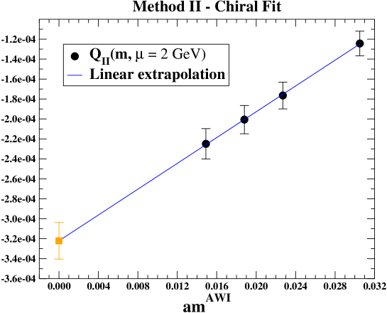
Notice that, in the chiral limit, $Q_{II}(x,m,\mu)$ reduces to $Q_{I}(x,\mu)$ defined in eq. (19). The small spread of the results coming from choosing the vector or the axial-vector quark masses is included in the systematics. We then fit $Q_{II}(x,m,\mu)$ either to a constant or linearly in $x^{2}$ and extrapolate the result, denoted as $Q_{II}(m,\mu)$ in fig. 7, to the chiral limit, where it reduces to the chiral quark condensate. The quark mass extrapolation is shown in fig. 7. Though the points in the plot look very well aligned, a quadratic fit in the quark mass has been also performed, in order to evaluate the corresponding systematic uncertainty. We find that the results obtained for the chiral quark condensate with this second approach are indistinguishable, within the statistical errors, from those derived by using the method I and presented in tab. 3.

6 Results and discussion

Our final estimate for the chiral quark condensate is obtained from the results given in table 3 after including the evaluation of the systematic error. We quote:

$$\langle\bar{\psi}\psi\rangle^{{\overline{\rm{MS}}}}(2\textrm{GeV})=-(265\pm 5\pm 22~{}\textrm{MeV})^{3}\,,$$ (23)

where the first error is statistical and the second systematic. The latter, which amounts to about 25%, is due to:

• the spread of the points in the fitting regions. As discussed in sect.3, this spread is mostly due to discretization effects which are left after the tree-level ${\cal O}(a)$-correction has been applied to the lattice data. This error, of about 18%, represents the main source of systematic uncertainty, besides the quenching approximation.

• Arbitrariness in the choice of the fitting interval (within the window $a\mathrel{\hbox to0.0pt{\raise 2.20013pt\hbox{$<$}\hss}{\lower 2.20013pt\hbox{$\sim$}}}x\mathrel{\hbox to0.0pt{\raise 2.20013pt\hbox{$<$}\hss}{\lower 2.20013pt\hbox{$\sim$}}}1/\Lambda_{\rm QCD}$). This yields a 4-5% uncertainty.

• Different functional forms considered in the fits. Performing a quadratic fit instead of a linear one in the quark mass extrapolations introduces a systematic difference of about 9%. Including the ${\cal O}(x^{2})$ contribution in the fits of $Q_{I}$ and $Q_{II}$ to their OPEs gives a 4-5% variation in the results.

• The statistical error associated to the determination of the lattice spacing. This error introduces an uncertainty of about 15% in the estimate of the quark condensate. Notice that the systematic error associated in the quenched approximation to the dependence of the lattice spacing on the physical quantity used to fix the scale is not included. We consider this error as a part of the systematic quenching effect.

• The uncertainty on the quark field renormalization constant $Z_{\psi}$, used to renormalize the quark propagator. This effect is completely negligible in the determination of the quark condensate, as discussed in sect.5.

• The difference between the results obtained using either the vector or the axial-vector definitions of the quark masses. The systematics is slightly affected by this effect, by less than 1%.

• The 10% error on the quenched estimate of $\Lambda_{\rm QCD}$ gives a completely negligible uncertainty in the determination of the quark condensate.

The uncertainty coming from finite volume effects cannot be directly estimated in the present study, since our results have been obtained at fixed volume. A study of lattice artifacts performed in ref. [15] has shown that in the short distance region, which is the one relevant for the $X$-space method, finite volume effects on the lattice correlation functions in the free theory are negligible with respect to discretization effects. We expect this result to remain valid in the interacting theory as well, though a more quantitative conclusion on this point would require further investigations. The main source of uncertainty which is not evaluated in our estimate of the chiral quark condensate is the effect of the quenching approximation.

In conclusion, in this exploratory study we have investigated on the lattice the OPE of the quark propagator at short euclidean distances, and shown the feasibility of this approach to compute the chiral quark condensate. The result obtained in this way is in good agreement with previous determinations of this quantity based on different approaches. The strategy investigated in the present study can be also applied to compute on the lattice the matrix elements of other local operators which enter the OPE of correlation functions at the leading orders. It can be also directly implemented in lattice simulations performed with dynamical quarks.

Appendix: NLO calculation of the Wilson coefficients

In this appendix we sketch the NLO QCD calculation of the Wilson coefficients introduced in eq. (6).

The OPE of the quark propagator in euclidean space is expressed by

$$T(\psi(x)\bar{\psi}(0)) = {\displaystyle{1\over 2\pi^{2}}}\,C_{I}(x)\,{\displaystyle{(\hbox to0.0pt{\hbox to5.71527pt{\hfil/\hfil}\hss}x)\over(x^{2})^{2}}}+{\displaystyle{1\over 4\pi^{2}}}\,C_{m}(x)\,{\displaystyle{m\over x^{2}}}$$ (24)

$$- {\displaystyle{1\over 4N}}\,C_{\bar{\psi}\psi}(x)\,(\bar{\psi}\psi)+\ldots$$

where the dots represent higher powers of $x^{2}$ and of the quark mass $m$. All quantities in eq. (24) are renormalized at a given scale and in a given renormalization scheme. In the following, we will choose the ${\overline{\rm{MS}}}$ renormalization scheme.

In order to determine the Wilson coefficients at the NLO in QCD, we calculate both the left and the right hand side of eq. (24) up to ${\cal O}(\alpha_{s})$ by choosing a common set of external states. The coefficients $C_{I}(x)$ and $C_{m}(x)$, in particular, can be determined by taking the vacuum expectation value of eq. (24) in perturbation theory, where the contribution of the quark condensate is vanishing. Eq. (24) then simply reduces to

$$S(x)={\displaystyle{1\over 2\pi^{2}}}\,C_{I}(x)\,{\displaystyle{(\hbox to0.0pt{\hbox to5.71527pt{\hfil/\hfil}\hss}x)\over(x^{2})^{2}}}+{\displaystyle{1\over 4\pi^{2}}}\,C_{m}(x)\,{\displaystyle{m\over x^{2}}}\,,$$ (25)

where $S(x)$ is the quark propagator computed in one-loop perturbation theory. By using dimensional regularization, with $D=4-2\varepsilon$, one has

$$S(x)=\displaystyle\int{\displaystyle{d^{D}\,k\over(2\pi)^{D}}}\,e^{-ik\cdot x}S(k)$$ (26)

where

$$S(k) = Z_{\psi}\,\frac{\hbox to0.0pt{\hbox to5.52084pt{\hfil/\hfil}\hss}k}{i\,k^{2}}\left[1-\frac{\alpha_{s}}{4\pi}\,C_{F}\,\xi\,\left({\displaystyle{k^{2}\over\mu^{2}}}\right)^{-\varepsilon}\left(\frac{1}{\hat{\varepsilon}}+1\right)\right]+$$ (27)

$$+ Z_{\psi}\,\frac{Z_{m}^{-1}\,m}{k^{2}}\left[1+\frac{\alpha_{s}}{4\pi}\,C_{F}\,\left({\displaystyle{k^{2}\over\mu^{2}}}\right)^{-\varepsilon}\left(\frac{3-\xi}{\hat{\varepsilon}}+4\right)\right]\,,$$

and $1/\hat{\varepsilon}\equiv 1/\varepsilon+\log(4\pi)-\gamma_{E}$. From eq. (27) one derives the expressions of the quark field and the quark mass renormalization constants in the ${\overline{\rm{MS}}}$ scheme:

$$Z_{\psi}=1+{\displaystyle{\alpha_{s}\over 4\pi}}\,C_{F}\,\frac{\xi}{\hat{\varepsilon}}\quad,\quad Z_{m}=1+{\displaystyle{\alpha_{s}\over 4\pi}}\,C_{F}\,\frac{3}{\hat{\varepsilon}}\,.$$ (28)

By inserting eq. (27) into eq. (26) and using

$$\int{\displaystyle{d^{D}\,k\over(2\pi)^{D}}}\frac{e^{-ik\cdot x}}{(k^{2})^{r}}={\displaystyle{1\over(4\pi)^{D/2}}}\,{\displaystyle{\Gamma(D/2-r)\over\Gamma(r)}}\left(\frac{x^{2}}{4}\right)^{r-D/2}$$ (29)

we obtain

$$S(x) = {\displaystyle{1\over 2\pi^{2}}}\left[1-{\displaystyle{\alpha_{s}\over 4\pi}}\,C_{F}\,\xi\left(2\gamma_{E}+\log(\mu^{2}x^{2}/4)\right)\right]{\displaystyle{(\hbox to0.0pt{\hbox to5.71527pt{\hfil/\hfil}\hss}x)\over(x^{2})^{2}}}+$$ (30)

$${\displaystyle{1\over 4\pi^{2}}}\left[1+{\displaystyle{\alpha_{s}\over 4\pi}}\,C_{F}\,\left(4-(\xi-3)\left(2\gamma_{E}+\log(\mu^{2}x^{2}/4)\right)\right)\right]{\displaystyle{m\over x^{2}}}\,.$$

From this result, after comparing with eq. (25), the Wilson coefficients $C_{I}(x)$ and $C_{m}(x)$ can be readily identified:

$$C_{I}(x) = 1-{\displaystyle{\alpha_{s}\over 4\pi}}\,C_{F}\,\xi\left[2\gamma_{E}+\log(\mu^{2}x^{2}/4)\right]$$

$$C_{m}(x) = 1+{\displaystyle{\alpha_{s}\over 4\pi}}\,C_{F}\,\left[4-(\xi-3)\left(2\gamma_{E}+\log(\mu^{2}x^{2}/4)\right)\right]\,.$$ (31)

In order to compute the Wilson coefficient of the quark condensate, $C_{\bar{\psi}\psi}(x)$, we derive a matching equation by inserting both sides of eq. (24) in a connected Green function with two external quark fields at fixed momenta:

$$\langle(\psi_{\alpha}^{a}(x)\bar{\psi}_{\beta}^{b}(0))\bar{\psi}_{\gamma}^{c}(p_{1})\psi_{\delta}^{d}(p_{2})\rangle=-\frac{1}{4N}\,\delta_{\alpha\beta}\delta^{ab}C_{\bar{\psi}\psi}(x)\,\langle(\bar{\psi}(0)\psi(0))\bar{\psi}_{\gamma}^{c}(p_{1})\psi_{\delta}^{d}(p_{2})\rangle\textrm{.}$$ (32)

By putting

$$C_{\bar{\psi}\psi}(x)=C^{0}_{\bar{\psi}\psi}(x)+\frac{\alpha_{s}}{4\pi}\,C^{1}_{\bar{\psi}\psi}(x)$$ (33)

and summing in eq. (32) over Dirac ($\alpha$,$\beta$) and color ($a$,$b$) indices, one immediately obtains the ${\cal O}(1)$ contribution to the Wilson coefficient,

$$C^{0}_{\bar{\psi}\psi}=1\,.$$ (34)

At ${\cal O}(\alpha_{s})$, the matching equation can be schematically written as

$$\langle(\bar{\psi}(0)\psi(x))\bar{\psi}\psi\rangle_{1}=C^{0}_{\bar{\psi}\psi}\langle(\bar{\psi}(0)\psi(0))\bar{\psi}\psi\rangle_{1}+C^{1}_{\bar{\psi}\psi}\langle(\bar{\psi}(0)\psi(0))\bar{\psi}\psi\rangle_{0}$$ (35)

where $\langle\ldots\rangle_{0}$ and $\langle\ldots\rangle_{1}$ represent respectively the ${\cal O}(1)$ and ${\cal O}(\alpha_{s})$ contributions to the Green functions. We now consider the amputated Green functions, and use eq. (34) together with the relation

$$\langle(\bar{\psi}(0)\psi(0))\bar{\psi}\psi\rangle_{0}^{amp}=I\,,$$ (36)

to obtain

$$C^{1}_{\bar{\psi}\psi}\cdot I=\langle(\bar{\psi}(0)\psi(x))\bar{\psi}\psi\rangle_{1}^{amp}-\langle(\bar{\psi}(0)\psi(0))\bar{\psi}\psi\rangle_{1}^{amp}\,.$$ (37)

The Feynman diagram which contributes to eq. (37) at ${\cal O}(\alpha_{s})$ is shown in fig. 8.

Figure 8: Feynman diagram relevant for the calculation of the Wilson coefficient $C_{\bar{\psi}\psi}(x)$ at ${\cal O}(\alpha_{s})$.

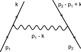
Since the matching condition is independent of the choice of the external states, we can evaluate this diagram by putting directly $p_{1}=p_{2}=0$. In addition, by having neglected in eq. (24) higher power corrections in the quark mass, we can compute the amputated Green functions in eq. (37) directly in the limit $m=0$. We then find:

$$C^{1}_{\bar{\psi}\psi}\cdot I = 16\,\pi^{2}C_{F}\,\mu^{2\varepsilon}\displaystyle\int{\displaystyle{d^{D}\,k\over(2\pi)^{D}}}\,\left(e^{-ik\cdot x}-1\right)\,\left[\gamma^{\mu}\frac{1}{\hbox to0.0pt{\hbox to5.52084pt{\hfil/\hfil}\hss}k}\frac{1}{\hbox to0.0pt{\hbox to5.52084pt{\hfil/\hfil}\hss}k}\gamma^{\nu}\right]\,\frac{1}{k^{2}}\left(\delta_{\mu\nu}-(1-\xi)\frac{k_{\mu}k_{\nu}}{k^{2}}\right)+$$ (38)

$$\left[\left(Z_{\psi}-1\right)-\left(Z_{\bar{\psi}\psi}-1\right)\right]\cdot I$$

where $Z_{\bar{\psi}\psi}=Z_{m}^{-1}$. By evaluating the Feynman integral with the aid of eq. (29), we finally obtain

$$C_{\bar{\psi}\psi}(x)=1+\frac{\alpha_{s}}{4\pi}\,C_{F}\left[2-(\xi+3)\left(2\gamma_{E}+\log(\mu^{2}x^{2}/4)\right)\right]$$ (39)

The complete NLO expressions for the Wilson coefficients are derived from eqs. (30) and (39) by applying the standard NLO evolution functions introduced in eq. (10).

References

- [1] P. Colangelo and A. Khodjamirian, arXiv:hep-ph/0010175.
- [2] H. G. Dosch and S. Narison, Phys. Lett. B 417, 173 (1998) [arXiv:hep-ph/9709215].
- [3] L. Giusti, F. Rapuano, M. Talevi and A. Vladikas, Nucl. Phys. B 538, 249 (1999) [arXiv:hep-lat/9807014].
- [4] S. Aoki et al. [CP-PACS Collaboration], Phys. Rev. D 67, 034503 (2003) [arXiv:hep-lat/0206009].
- [5] L. Giusti, C. Hoelbling and C. Rebbi, Phys. Rev. D 64, 114508 (2001) [Erratum-ibid. D 65, 079903 (2002)] [arXiv:hep-lat/0108007].
- [6] P. Hernandez, K. Jansen, L. Lellouch and H. Wittig, JHEP 0107, 018 (2001) [arXiv:hep-lat/0106011].
- [7] P. Hernandez, K. Jansen and L. Lellouch, Phys. Lett. B 469, 198 (1999) [arXiv:hep-lat/9907022].
- [8] P. Hasenfratz, S. Hauswirth, T. Jorg, F. Niedermayer and K. Holland, Nucl. Phys. B 643, 280 (2002) [arXiv:hep-lat/0205010].
- [9] T. DeGrand [MILC Collaboration], Phys. Rev. D 64, 117501 (2001) [arXiv:hep-lat/0107014].
- [10] J. R. Cudell, A. Le Yaouanc and C. Pittori, Phys. Lett. B 454, 105 (1999) [arXiv:hep-lat/9810058].
- [11] D. Becirevic and V. Lubicz, Phys. Lett. B 600 (2004) 83 [arXiv:hep-ph/0403044].
- [12] K.G. Wilson, Phys. Rev. Suppl. 179, (1969) 1499.
-
[13]
V. A. Novikov, M. A. Shifman, A. I. Vainshtein, M. B. Voloshin and V. I. Zakharov,
Nucl. Phys. B 237, 525 (1984).
M. A. Shifman, A. I. Vainshtein and V. I. Zakharov, Nucl. Phys. B 147, 385 (1979). - [14] D. Becirevic, V. Gimenez, V. Lubicz and G. Martinelli, Phys. Rev. D 61 (2000) 114507 [arXiv:hep-lat/9909082].
- [15] V. Gimenez et al., Phys. Lett. B 598 (2004) 227 [arXiv:hep-lat/0406019].
- [16] G. Martinelli, G. C. Rossi, C. T. Sachrajda, S. R. Sharpe, M. Talevi and M. Testa, Phys. Lett. B 411 (1997) 141 [arXiv:hep-lat/9705018].
- [17] D. Becirevic, V. Gimenez, V. Lubicz, G. Martinelli, M. Papinutto and J. Reyes, JHEP 0408, 022 (2004) [arXiv:hep-lat/0401033].
- [18] P. Pascual and E. de Rafael, Z. Phys. C 12, (1982) 127.
- [19] D. Becirevic, V. Lubicz and C. Tarantino [SPQ(CD)R Collaboration], Phys. Lett. B 558, 69 (2003) [arXiv:hep-lat/0208003].
- [20] S. Necco and R. Sommer, Nucl. Phys. B 622, 328 (2002) [arXiv:hep-lat/0108008].
- [21] S. Capitani, M. Luscher, R. Sommer and H. Wittig [ALPHA Collaboration], Nucl. Phys. B 544, 669 (1999) [arXiv:hep-lat/9810063].