DESY 05-009 Edinburgh 2005/01 LU-ITP 2005/006 Generalized parton distributions and transversity from full lattice QCD

Abstract

We present here the latest results from the QCDSF collaboration for moments of generalized parton distributions and transversity in two-flavour QCD, including a preliminary analysis of the pion mass dependence.

1 INTRODUCTION

For many years deep-inelastic scattering experiments have provided a wealth of information regarding the quark and gluon content of the nucleon, mainly through parton distribution functions which describe the longitudinal momentum distributions of quarks and gluons in the nucleon. Although the amount of knowledge gained from such experiments is constantly increasing, little is known about the transverse structure and angular momentum distribution of partons within the nucleon. Generalized parton distributions (GPDs) [1] have opened new ways of studying the complex interplay of longitudinal momentum and transverse coordinate space [2, 3], as well as spin and orbital angular momentum degrees of freedom in the nucleon [4]. A full mapping of the parameter space spanned by GPDs is an extremely extensive task which most probably needs support from non-perturbative techniques like lattice simulations.

Besides the polarized and unpolarized GPDs, there exist also four independent tensor/helicity flip GPDs $H_{T}(x,\xi,t),E_{T},\widetilde{H}_{T}$ and $\widetilde{E}_{T}$, as has been shown in [5]. The first one, $H_{T}(x,\xi,t)$, is called generalized transversity, because it reproduces the transversity distribution in the foward limit, $H_{T}(x,0,0)=\delta q(x)=h_{1}(x)$. Since the quark tensor GPDs flip the helicity of the quarks, they do not contribute to the deeply virtual Compton scattering (DVCS) process $\gamma^{*}p\rightarrow\gamma p^{\prime}$. Although this could in principle be balanced by the production of a transversely polarized vector meson, $\gamma^{*}p\rightarrow m_{T}p^{\prime}$, it has been shown that the corresponding amplitude vanishes at leading twist to all orders in perturbation theory [6, 7, 8]. The only process we are currently aware of which gives access to the generalized transversity is the diffractive double meson production proposed in [9]. It will be very interesting to see if a measurement of tensor GPDs in this process is indeed feasible. In any case, the situation seems to be much more difficult as compared to the (un-)polarized GPDs, and an independent lattice calculation of the moments of the helicity flip GPDs would be highly valuable.

There has been a large amount of activity within the lattice community in the area of GPDs leading to some exciting results from the QCDSF [10, 11, 12, 13] and LHP [14, 15, 16, 17, 18, 19] collaborations.

Here we present the latest results from the QCDSF collaboration for the first three moments of the unpolarized and polarized GPDs and results for the tranversity GPDs. All results are preliminary.

2 SIMULATION DETAILS

We simulate with $N_{\rm f}=2$ dynamical configurations generated with Wilson glue and non-perturbatively ${\cal O}(a)$ improved Wilson fermions. For five different values $\beta=5.20$, $5.25$, $5.26$, $5.29$, $5.40$ and up to three different kappa values per beta we have in collaboration with UKQCD generated ${\cal O}(2000-8000)$ trajectories. Lattice spacings and spatial volumes vary between 0.075-0.123 fm and (1.5-2.2 fm)³ respectively.

Correlation functions are calculated on configurations taken at a distance of 5-10 trajectories using 8-4 different locations of the fermion source. We use binning to obtain an effective distance of 20 trajectories. The size of the bins has little effect on the error, which indicates auto-correlations are small. This work improves on previous calculations by adding one more sink momentum, $\vec{p}_{2}$, and polarization, $\Gamma_{1}$. We use $\vec{p}_{0}=(0,0,0)$, $\vec{p}_{1}=(p,0,0)$, $\vec{p}_{2}=(0,p,0)$ ($p=2\pi/L_{S}$) and $\Gamma_{\rm unpol}=\frac{1}{2}(1+\gamma_{4})$, $\Gamma_{1}=\frac{1}{2}(1+\gamma_{4})\,i\gamma_{5}\gamma_{1}$, $\Gamma_{2}=\frac{1}{2}(1+\gamma_{4})\,i\gamma_{5}\gamma_{2}$.

3 GENERALIZED PARTON DISTRIBUTIONS

For a lattice calculation of GPDs, we work in Mellin-space to relate matrix elements of local operators to Mellin moments of the GPDs. For quark distributions, the twist-2 operators are

$${\cal O}^{\{\mu_{1}\cdots\mu_{n}\}} = \overline{q}\,i\,\gamma^{\{\mu_{1}}\,\stackrel{{\scriptstyle\leftrightarrow}}{{D}}^{\mu_{2}}\cdots\stackrel{{\scriptstyle\leftrightarrow}}{{D}}^{\mu_{n}\}}\!q\ ,$$ (1)

$$\widetilde{{\cal O}}^{\{\mu_{1}\cdots\mu_{n}\}} = \overline{q}\,i\,\gamma^{5}\gamma^{\{\mu_{1}}\,\stackrel{{\scriptstyle\leftrightarrow}}{{D}}^{\mu_{2}}\cdots\stackrel{{\scriptstyle\leftrightarrow}}{{D}}^{\mu_{n}\}}\!q\ ,$$ (2)

$${\cal O}_{T}^{[\rho\{\mu_{1}]\cdots\mu_{n}\}} = \overline{q}\,i\,\gamma^{5}\sigma^{\rho\{\mu_{1}}\gamma^{\mu_{2}}\,\stackrel{{\scriptstyle\leftrightarrow}}{{D}}^{\mu_{3}}\cdots\stackrel{{\scriptstyle\leftrightarrow}}{{D}}^{\mu_{n}\}}\!q\ ,$$ (3)

where $\stackrel{{\scriptstyle\leftrightarrow}}{{D}}=\frac{1}{2}(\overrightarrow{D}-\overleftarrow{D})$ and $\{\cdots\}$ indicates symmetrization of indices and removal of traces. The non-forward matrix elements of the twist-2 operators Eqs. (1, 2, 3) specify the $(n-1)^{th}$ moments of the spin-averaged, spin-dependent and spin-flip generalized parton distributions, respectively. In particular, for the unpolarized GPDs, we have

$$\!\!\int_{-1}^{1}dx\,x^{n-1}\,H^{q}(x,\xi,\Delta^{2})\!\! = \!\!H^{q}_{n}(\xi,\Delta^{2})\ ,$$

$$\!\!\int_{-1}^{1}dx\,x^{n-1}\,E^{q}(x,\xi,\Delta^{2})\!\! = \!\!E^{q}_{n}(\xi,\Delta^{2})\ ,$$ (4)

where [4]

$$H^{q}_{n}(\xi,\Delta^{2}) = \sum_{i=0}^{\frac{n-1}{2}}A^{q}_{n,2i}(\Delta^{2})(-2\xi)^{2i}+{\rm Mod}(n+1,2)C^{q}_{n}(\Delta^{2})(-2\xi)^{n}\ ,$$

$$E^{q}_{n}(\xi,\Delta^{2}) = \sum_{i=0}^{\frac{n-1}{2}}B^{q}_{n,2i}(\Delta^{2})(-2\xi)^{2i}-{\rm Mod}(n+1,2)C^{q}_{n}(\Delta^{2})(-2\xi)^{n}\ ,$$ (5)

and the generalized form factors $A^{q}_{n,2i}(\Delta^{2})$, $B^{q}_{n,2i}(\Delta^{2})$ and $C^{q}_{n}(\Delta^{2})$ for the lowest three moments are extracted from the nucleon matrix elements $\langle p^{\prime}|{\cal O}^{\{\mu_{1}\cdots\mu_{n}\}}|p\rangle$ [4]. Note that the momentum transfer is given by $\Delta=p^{\prime}-p$ with $t=\Delta^{2}$, while $\xi=-n\cdot\Delta/2$ denotes the longitudinal momentum transfer. For the lowest moment, $A_{10}$ and $B_{10}$ are just the Dirac and Pauli form factors $F_{1}$ and $F_{2}$, respectively. We also observe that in the forward limit ($\Delta^{2}=\xi=0$), the moments of $H_{q}$ reduce to the moments of the unpolarized parton distribution $A_{n0}=\langle x^{n-1}\rangle$. Finally, the forward limit of the $x$-moment of the GPD $E$, $\int dx\,x\,E(x,0,0)=B_{20}(0)$, allows for the determination of the quark orbital angular momentum contribution to the nucleon spin, $L^{q}=1/2(\langle x\rangle+B_{20}-\Delta q)$, where $\langle x\rangle$ is the quark momentum fraction [4].

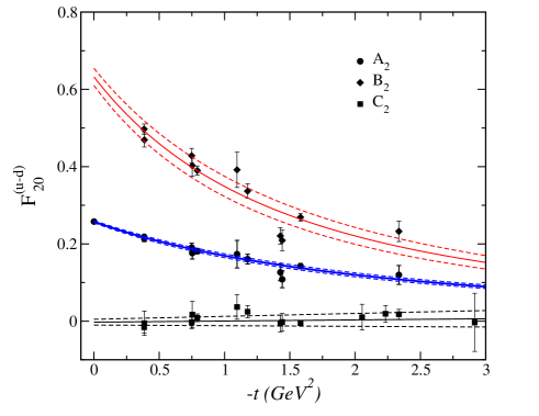
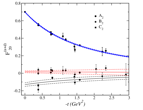
Figure 1: Generalized form factors $A_{20},\ B_{20}$ and $C_{2}$, together with a dipole fit for the non-singlet, $u-d$ (left), and singlet, $u+d$ (right).

In order to extract the non-forward matrix elements we compute ratios of three- and two-point functions

$$R(t,\tau;\vec{p}\,^{\prime},\vec{p};{\cal O})\, = \frac{C_{\Gamma}(t,\tau;\vec{p}\,^{\prime},\vec{p},{\cal O})}{C_{2}(t,\vec{p}\,^{\prime})}\left[\frac{C_{2}(\tau,\vec{p}\,^{\prime})C_{2}(t,\vec{p}\,^{\prime})C_{2}(t-\tau,\vec{p})}{C_{2}(\tau,\vec{p})C_{2}(t,\vec{p})C_{2}(t-\tau,\vec{p}\,^{\prime})}\right]^{\frac{1}{2}}$$

$$\propto \ \langle p^{\prime}|{\cal O}_{q}|p\rangle\ ,$$

up to known kinematical factors as long as $0\ll\tau\ll t\lesssim\frac{1}{2}L_{T}$.

In Fig. 1 we show, as an example, the generalized form factors $A_{20},\ B_{20}$ and $C_{2}$ in the $\overline{\rm MS}$ scheme at $\mu^{2}=4$ GeV² for the non-singlet, $u-d$ (left), and singlet, $u+d$ (right), on a $24^{3}\times 48$ lattice at $\beta=5.40$ and $\kappa_{\rm sea}=\kappa_{\rm val}=0.13500$ corresponding to a lattice spacing, $a\,r_{0}=6.088$ and $m_{\pi}=m_{\rm PS}\approx 970$ MeV. We note here that in the calculation of the singlet matrix elements, we neglect contributions coming from disconnected quark diagrams as these are extremely computationally demanding.

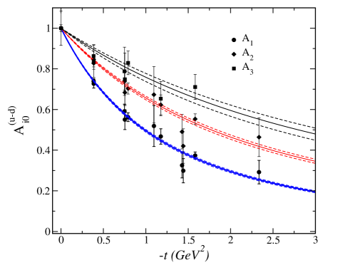
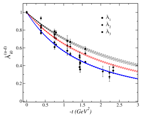
Figure 2: Generalized form factors $A^{u-d}_{10},\ A^{u-d}_{20}$, $A^{u-d}_{30}$ (left), and $\widetilde{A}^{u-d}_{10},\ \widetilde{A}^{u-d}_{20}$, $\widetilde{A}^{u-d}_{30}$ (right), together with a dipole fit. All form factors have been normalized to unity.

The generalized form factors $A^{u-d}_{20},\ A^{u+d}_{20}$ and $B^{u-d}_{20}$ are well described by the dipole ansatz

$$A_{n}^{q}(\Delta^{2})=\frac{A_{n}^{q}(0)}{\big{(}1-{\Delta^{2}/M_{n}^{2}}\big{)}^{2}}\ ,$$ (7)

while $C^{u-d}_{2}$ is consistent with zero. Our result for $B^{u+d}_{2}$ reveals a small but positive value at this heavy quark mass. Future work will include a full non-perturbative analysis of $\Delta q^{u+d}$ and $\Delta q^{u-d}$, together with a chiral extrapolation, to reveal the quark contributions to the nucleon’s total spin and orbital angular momentum.

Burkardt [3] has shown that the spin-independent and spin-dependent generalized parton distributions $H(x,0,\Delta^{2})$ and $\widetilde{H}(x,0,\Delta^{2})$ gain a physical interpretation when Fourier transformed to impact parameter space at longitudinal momentum transfer $\xi=0$

$$q(x,\vec{b}_{\perp})=\int\frac{d^{2}\Delta_{\perp}}{(2\pi)^{2}}\,{\rm e}^{-i\vec{b}_{\perp}\cdot\vec{\Delta}_{\perp}}H(x,0,-\Delta_{\perp}^{2})\,,$$ (8)

(and similar for the polarized $\Delta q(x,\vec{b}_{\perp})$) where $q(x,\vec{b}_{\perp})$ is the probability density for a quark with longitudinal momentum fraction $x$ and at transverse position (or impact parameter) $\vec{b}_{\perp}$.

Burkardt [3] also argued that $H(x,0,-\Delta_{\perp}^{2})$ becomes $\Delta_{\perp}^{2}$-independent as $x\rightarrow 1$ since, physically, we expect the transverse size of the nucleon to decrease as $x$ increases, i.e. $\lim_{x\rightarrow 1}q(x,\vec{b}_{\perp})\propto\delta^{2}(\vec{b}_{\perp})$. As a result, we expect the slopes of the moments of $H(x,0,-\Delta_{\perp}^{2})$ in $\Delta_{\perp}^{2}$ to decrease as we proceed to higher moments. This is also true for the polarized moments of $\widetilde{H}(x,0,-\Delta_{\perp}^{2})$, so from Eq. (5) with $\xi=0$, we expect that the slopes of the generalized form factors $A_{n0}(\Delta^{2})$ and $\widetilde{A}_{n0}(\Delta^{2})$ should decrease with increasing $n$.

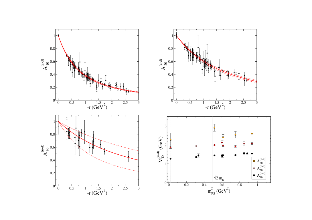
Figure 3: Generalized form factors $A^{u-d}_{10},\ A^{u-d}_{20}$ and $A^{u-d}_{30}$, together with a dipole fit. All form factors have been normalized to unity. Dipole masses are extrapolated linearly to the chiral limit.

In Fig. 2, we show the $\Delta^{2}$-dependence of $A_{n0}(\Delta^{2})$ (left) and $\widetilde{A}_{n0}(\Delta^{2})$ (right), $n=1,2,3$, for $\beta=5.40$, $\kappa_{\rm sea}=\kappa_{\rm val}=0.13500$. The form factors have been normalized to unity to make a comparison of the slopes easier and as in Fig. 1 we fit the form factors with a dipole form as in Eq. (7). We observe here that the form factors for the unpolarized moments are well separated and that their slopes do indeed decrease with increasing $n$ as predicted. For the polarized moments, we observe a similar scenario, however here the change in slope between the form factors is not as large. The flattening of the GFFs $A_{n0}(\Delta^{2})$ has first been observed in Ref. [15], where at the same time practically no change in slope has been seen going from $\widetilde{A}_{20}(\Delta^{2})$ to $\widetilde{A}_{30}(\Delta^{2})$.

Although fitting the form factors with a dipole is purely phenomenological, (see Ref. [20] for an alternative ansatz) it does provide us with a useful means to measure the change in slope of the form factors by monitoring the extracted dipole masses $(M_{1},\,M_{2},\,M_{3})$ as we proceed to higher moments. We have calculated these generalized form factors on a subset of our full complement of $(\beta,\,\kappa)$ combinations and have extracted the corresponding dipole masses. We plot these dipole masses in the lower-right of Fig. 3 as a function of $m_{\rm PS}^{2}$. The values quoted in the chiral limit are calculated via a combined dipole-mass/pion-mass fit

$$\bar{A}_{n0}^{\text{dipole},m_{\pi}}(\Delta^{2})=\frac{1}{\left(1-{t/(M_{D}^{0}+\alpha m_{\pi}^{2})^{2}}\right)^{2}}\ ,$$ (9)

depending on the two parameters $M_{D}^{0}$ and $\alpha$, in order to extract the maximum amount of information from our available $(\beta,\,\kappa)$ combinations. Having done the fit, we may shift the raw numbers to a common curve given by Eq.(9) at the physical pion mass, $m_{\pi,\text{phys}}=139$ MeV. The results of this procedure are shown in Fig. 3 for the GFFs $A_{n0}$, $n=1,2,3$.

The important feature to note in Fig. 3 is the distinct separation between (and increase in magnitude of) the dipole masses as we move to higher moments $(x\rightarrow 1)$. Although the data available for $M_{3}$ is limited, the behaviour of all dipole masses appears to be linear with $m_{\rm PS}^{2}$. Consequently, we perform individual linear extrapolations of the dipole masses $M_{1},\,M_{2},\,M_{3}$ to the physical pion mass, although the findings of Ref. [21] suggest that the chiral extrapolation of the dipole masses of the electromagnetic form factors may be non-linear.

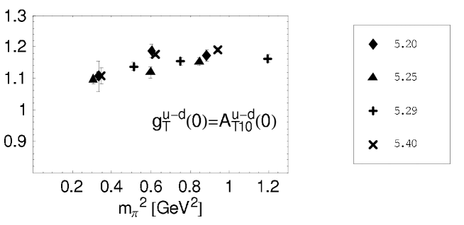
Figure 4: The iso-vector tensor charge vs. $m_{\pi}^{2}$.

If the dipole behavior Eq. (7) continues to hold for the higher moments as well, and if we assume that the dipole masses continue to grow in a Regge-like fashion, we may write

$$\int_{-1}^{1}\mbox{d}x\,x^{n-1}\,H_{q}(x,0,\Delta^{2})=\frac{\langle x_{q}^{n-1}\rangle}{(1-\Delta^{2}/M_{n}^{2})^{2}},$$ (10)

with $M_{l}^{2}=\mbox{const.}+l/\alpha^{\prime}$, where $\mbox{const.}\approx-0.5$ GeV² and $1/\alpha^{\prime}\approx 1.1$ GeV². This is sufficient to compute $H_{q}(x,0,\Delta^{2})$ by means of an inverse Mellin transform [22].

Having done so, the desired probability distribution of finding a parton of momentum fraction $x$ at the impact parameter $\vec{b}_{\perp}$ can then be obtained by the Fourier transform of Eq. (8).

We now turn our attention to our latest results for the first two moments of the tensor GPDs. Since the parameterizations for the Mellin-transformed tensor GPDs have been derived recently in [23, 24] in terms of the GFFs $A_{Tni},\widetilde{A}_{Tni},B_{Tni}$ and $\widetilde{B}_{Tni}$, we are now in a position which allows for the extraction of the moments of $H_{T}(x,\xi,t)$ etc. from our lattice calculation. The lowest moment of the generalized transversity, $\int dxH_{T}(x,\xi,t)=A_{T10}(\Delta^{2})$, is equal to the tensor form factor $g_{T}(\Delta^{2})=A_{T10}(\Delta^{2})$. Our results for the iso-vector tensor charge, $g^{3}_{T}(0)$, are shown in Fig. 4 as a function of the pion mass squared. The lattice results for $g^{3}_{T}$ have been non-perturbatively renormalized and transformed to the $\overline{\rm MS}$ scheme at $Q^{2}=4$ GeV². The plot indicates that sizeable discretization and/or finite volume effects may be present which we will study in detail in the near future. A linear extrapolation of the isovector tensor charge to the physical pion mass gives $g^{3}_{T}(0)=1.09\pm 0.02$. A more advanced form for the chiral extrapolation of $g^{3}_{T}$ including effects from the pion cloud is also currently under investigation [25, 26].

Fig. 5 shows combined dipole-/pion-mass-fits of $g^{3}_{T}(\Delta^{2})$ and the $n=2$ -moment of the generalized transversity, $A_{T20}(\Delta^{2})$, following Eq.(9). The corresponding dipole masses and fit-parameters are given by

$$A_{T10}\, : \,M_{D}^{0}=1.63\!\pm\!.02\text{ GeV},\,\,\,\alpha=0.10\!\pm\!.03\text{ GeV}^{-2},\,\,\,\chi^{2}/\text{DOF}=1.1$$

$$A_{T20}\, : \,M_{D}^{0}=2.17\!\pm\!.04\text{ GeV},\,\,\,\alpha=-0.06\!\pm\!.06\text{ GeV}^{-2},\,\,\,\chi^{2}/\text{DOF}=0.9,$$ (11)

showing an increase in the dipole mass, going from the $n=1$ to the $n=2$-Mellin-moment. The errors in Eq. (11) are purely statistical. Results for the other tensor GFFs $\widetilde{A}_{Tn0},B_{Tn0}$ and $\widetilde{B}_{Tn0}$ for $n=1,2$ will be presented in a future publication. For the tensor GPDs, the number $N$ of GFFs grows rapidly with $n$, i.e. $N=2\lceil n/2\rceil+n$. For $n=3$ we would have to extract simultaneously seven independent GFFs from the lattice, which poses quite a challenge. We plan to study the relevant two-derivative tensor operators on the lattice to see if and to what extent an extraction is possible.

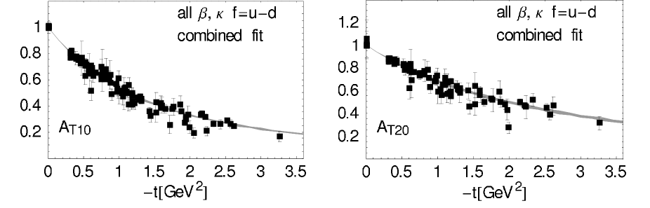
Figure 5: Combined dipole-/pion-mass fits to the generalized form factors $A_{T10}$ and $A_{T20}$.

References

- [1] D. Müller et al., Fortsch. Phys. 42, 101 (1994); A.V. Radyushkin, Phys. Rev. D 56, 5524 (1997); M. Diehl et al., Phys. Lett. B 411, 193 (1997).
- [2] M. Diehl, Eur. Phys. J. C 25, 223 (2002).
- [3] M. Burkardt, Int. J. Mod. Phys. A 18, 173 (2003).
- [4] X. Ji, Phys. Rev. Lett. 78, 610 (1997); X. Ji, J. Phys. G 24, 1181 (1998).
- [5] M. Diehl, Eur. Phys. J. C 19 (2001) 485.
- [6] L. Mankiewicz, G. Piller and T. Weigl, Eur. Phys. J. C 5 (1998) 119.
- [7] M. Diehl, T. Gousset and B. Pire, Phys. Rev. D 59 (1999) 034023.
- [8] J. C. Collins and M. Diehl, Phys. Rev. D 61 (2000) 114015.
- [9] D. Y. Ivanov et al., Phys. Lett. B 550 (2002) 65.
- [10] M. Göckeler et al., Phys. Rev. Lett. 92, 042002 (2004).
- [11] T. Bakeyev et al., Nucl. Phys. Proc. Suppl. 128, 82 (2004).
- [12] M. Göckeler et al., hep-lat/0409162.
- [13] M. Göckeler et al., hep-lat/0410023.
- [14] Ph. Hägler et al., Phys. Rev. D 68 (2003) 034505.
- [15] Ph. Hägler et al., Phys. Rev. Lett. 93 (2004) 112001.
- [16] D. B. Renner et al., hep-lat/0409130.
- [17] Ph. Hägler et al., hep-ph/0410017.
- [18] Talk by W. Schroers, these proceedings.
- [19] D. B. Renner, hep-lat/0501005.
- [20] M. Diehl, T. Feldmann, R. Jakob and P. Kroll, hep-ph/0408173.
- [21] J.D. Ashley et al., Eur. Phys. J. A 19, 9 (2004).
- [22] M. Göckeler et al., hep-ph/9711245.
- [23] Ph. Hägler, Phys. Lett. B 594 (2004) 164.
- [24] Z. Chen and X. D. Ji, hep-ph/0404276.
- [25] A. A. Khan et al., hep-lat/0409161.
- [26] M. Göckeler et al., in preparation.
- [27] C. R. Allton et al., Phys. Rev. D 65 (2002) 054502.