ADP-05-02/T612
JLAB-THY-05-294
Extrapolation of lattice QCD results beyond the power-counting regime

Abstract

Resummation of the chiral expansion is necessary to make accurate contact with current lattice simulation results of full QCD. Resummation techniques including relativistic formulations of chiral effective field theory and finite-range regularization (FRR) techniques are reviewed, with an emphasis on using lattice simulation results to constrain the parameters of the chiral expansion. We illustrate how the chiral extrapolation problem has been solved and use FRR techniques to identify the power-counting regime (PCR) of chiral perturbation theory. To fourth-order in the expansion at the 1% tolerance level, we find $0\leq m_{\pi}\leq 0.18$ GeV for the PCR, extending only a small distance beyond the physical pion mass.

1 INTRODUCTION

Dynamical chiral symmetry breaking in QCD gives rise to an octet of light mesons recognized as the (pseudo) Goldstone bosons of the symmetry. These light mesons couple strongly and give rise to a quark-mass dependence of hadron observables which is nonanalytic in the quark mass. The Adelaide Group has played a leading role in emphasizing the role of this physics in the chiral extrapolation of lattice simulation results [1, 2, 3, 4, 5, 6, 7]. Most work in the baryon sector has focused on the nucleon and Delta masses and the magnetic moments of octet baryons.

The established, model-independent approach to chiral effective field theory is that of power counting, the foundation of chiral perturbation theory ($\chi$PT). However, this requires one to work in a regime of pion mass where the next term in the truncated series expansion makes a contribution that is negligible. Given the emphasis on determining the nucleon mass to 1%, such neglected contributions must be constrained to the fraction of a percent level. As there is no attempt to model the higher-order terms of the chiral expansion, one simply obtains the wrong answer if one works outside this region.

There is now growing recognition that some form of resummation of the chiral expansion is necessary in order to make contact with lattice simulation results of full QCD, where the effects of dynamical fermions are incorporated. As we will demonstrate in the following, the quark masses accessible with today’s algorithms and supercomputers lie well outside the regime of $\chi$PT in its standard form. This situation is unlikely to change significantly until it becomes possible to directly simulate QCD on the lattice within twice the squared physical mass of the pion and with suitably large lattice volumes. Within this range, knowledge of the first few terms of the chiral expansion would be sufficient as higher-order terms of the expansion are small simply because $m_{\pi}$ is small. Straightforward application of the truncated expansion of $\chi$PT would then be possible. However, one might wonder if the lattice techniques that would allow simulations at light masses within $2m_{\pi}^{2}$, might also allow a calculation directly at the physical pion mass, obliterating the chiral extrapolation problem altogether. Unfortunately such simulations are not possible in the foreseeable future, and one must resort to more advanced techniques.

The resummation of the chiral expansion induced through the introduction of a finite-range cutoff in the momentum-integrals of meson-loop diagrams is perhaps the best known resummation method [3, 4, 5, 6, 7, 8, 9, 10] — for alternative proposals, see also Refs. [11, 12]. However, there are many ways of regularizing the loop integrals which lead to a resummation of the expansion. For example, relativistic formulations lead to expressions for the nucleon self-energy which include higher-order nonanalytic terms beyond the order one is calculating [13]. In some cases, the expressions have the desirable property of becoming smooth and slowly varying as the pion mass becomes moderately large [14]. Indeed all observables calculated on the lattice display a smooth slowly-varying dependence on the quark mass, presenting a clear signal that higher order terms of the chiral expansion sum to zero as the pion mass becomes moderately large.

The ability to draw a curve through the lightest nucleon mass points has led some to argue that it is essential to adopt a relativistic approach in calculating the chiral expansion [13, 15]. However, one might have some concern that a relativistic expression is so important in what is supposed to be a low-energy effective field theory. Indeed, a Taylor expansion of the relativistic expression produces exactly the same leading-nonanalytic (LNA) term as obtained in the heavy-baryon formulation of chiral perturbation theory (HB$\chi$PT). Upon including the Delta in HB$\chi$PT the next-to-leading nonanalytic (NLNA) structure, $m_{\pi}^{4}\log m_{\pi}$ is also obtained.

In the relativistic formulation, an $m_{\pi}^{5}$ correction is also generated at one-loop order. However, the rapid convergence of the Taylor series generated by the full relativistic loop calculation [13] emphasizes that the relativistic corrections are small. One should not assume that the higher-order terms of the heavy-baryon expansion are included completely. Rather a particular resummation of the chiral expansion has been obtained which allows the self-energy of the nucleon to evolve slowly as the pion mass grows, thus mimicking the lattice simulation results.

Perhaps the most astonishing discovery in FRR chiral effective field theory, is that the term-by-term details of the higher-order chiral expansion are largely irrelevant in describing the chiral extrapolation of simulation results. Figure 1 displays the extrapolation [5] of lattice simulation results of full QCD from the CP-PACS collaboration [16]. A variety of finite-range regularizations are illustrated, including dipole, monopole, Gaussian and theta-function regulators, as described in greater detail below. FRR chiral effective field theory is mathematically equivalent to $\chi$PT to any finite order and in this case we work to order $m_{\pi}^{4}\log m_{\pi}$.

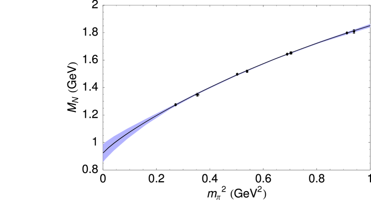
Figure 1: Extrapolation of CP-PACS collaboration simulation results [16] to the chiral limit using finite-range regularization [5]. Differences between the illustrated dipole, monopole, Gaussian and theta-function regulators cannot be resolved on this scale. The one-standard deviation error bound for the dipole extrapolation is also illustrated.

The curves are indistinguishable and produce physical nucleon masses which differ by less than 0.1%. This is despite the fact that the coefficients of the higher-order terms ($m_{\pi}^{5}$ and beyond) appearing in the FRR expressions differ significantly. For example, the coefficient of the $m_{\pi}^{5}$ term vanishes for the theta-function regulator, whereas the monopole, dipole and Gaussian regulators provide $-44$, $-34$ and $-30\,{\rm GeV}^{-4}$ respectively. What these expansions do have in common is that the loop-integrals vanish as the quark masses grow large. The contribution of any individual higher-order term is largely irrelevant. The only thing that really counts is that there are other terms that enter to ensure the sum of all terms of the loop integral approaches zero, in accord with what is observed in lattice QCD calculations. Of course, this beautiful feature of FRR expansions would be lost if one were to truncate the expansion at any finite order. Resummation of chiral effective field theory is essential to solving the chiral extrapolation problem.

In each of the aforementioned regulators, there is a single parameter governing the range of the loop-momentum cutoff. It is a parameter which does not appear in standard chiral perturbation theory and as outlined in detail below it plays no role in the terms of the FRR expansion to the order one is working. However, it does play a role in determining the coefficients of the higher-order terms, beyond that order. As discussed in detail in Ref. [5], it governs the convergence properties of the chiral expansion. Given the level of agreement between the curves associated with different regulators, it is sufficient to parameterize the remainder of the chiral expansion in terms of this single parameter, $\Lambda$, and still maintain fraction of a percent accuracy.

It is essential that $\Lambda$ remain finite. In the limit $\Lambda\to\infty$ one recovers the standard chiral expansion of $\chi$PT truncated at the next nonanalytic term beyond the order one is working, spoiling the resummation of the expansion. $\Lambda$ must be constrained to values that ensure that the loop-momenta contributing to loop integrals are relevant to the low-energy effective field theory. Indeed it is the erroneous contributions from large loop-momenta beyond the realm of the low-energy effective field theory that spoils the convergence properties of traditional $\chi$PT [8]. The difficulty with this approach is that the exact value of $\Lambda$ is not specified. Because one must work to finite order in the expansion, there is a residual dependence on $\Lambda$. The common approach is to vary $\Lambda$ over reasonable values and include the observed variation in the final uncertainty estimate.

2 FORMAL BACKGROUND

In the usual formulation of effective field theory, the nucleon mass as a function of the pion mass (given that $m_{\pi}^{2}\propto m_{q}$) has the formal expansion:

$$M_{N}=a_{0}+a_{2}m_{\pi}^{2}+a_{4}m_{\pi}^{4}+a_{6}m_{\pi}^{6}+\chi_{\pi}I_{\pi}+\chi_{\pi\Delta}I_{\pi\Delta}+\chi_{\rm tad}I_{\rm tad}\,.$$ (1)

In practice, for current applications to lattice QCD, the parameters, $a_{i}$, should be determined by fitting to the lattice results themselves. The additional terms, $\chi_{\pi}I_{\pi}$, $\chi_{\pi\Delta}I_{\pi\Delta}$ and $\chi_{\rm tad}I_{\rm tad}$, are loop corrections involving the (Goldstone) pion. As these terms involve the coupling constants in the chiral limit, which are essentially model-independent [18], the only additional complication they add is that the ultra-violet behavior of the loop integrals must be regulated in some way.

Traditionally, one uses dimensional regularization which (after infinite renormalization of $a_{0}$ and $a_{2}$) leaves only the non-analytic terms — $c_{\rm LNA}m_{\pi}^{3}$ and $c_{\rm NLNA}m_{\pi}^{4}\ln(m_{\pi}/\mu)$, respectively. Within dimensional regularization one then arrives at a truncated power series for the chiral expansion. To fourth order

$$M_{N}=c_{0}+c_{2}m_{\pi}^{2}+c_{\rm LNA}m_{\pi}^{3}+c_{4}m_{\pi}^{4}+c_{\rm NLNA}m_{\pi}^{4}\log\frac{m_{\pi}}{\mu}+c_{6}^{\prime}m_{\pi}^{6}\,,$$ (2)

where the bare parameters, $a_{i}$, have been replaced by the finite, renormalized coefficients, $c_{i}$. Through the chiral logarithm one has an additional mass scale, $\mu$, but the dependence on this is eliminated by matching $c_{4}$ to “data” (in this case lattice QCD). The prime on $c_{6}^{\prime}$ denotes that this term is beyond the order to which we are working, and therefore should not be expected to be independent of regularization.

In line with the implicit $\mu$-dependence of the coefficients in the familiar dimensionally regulated $\chi$PT, the systematic FRR expansion of the nucleon mass is:

$$M_{N}=a_{0}^{\Lambda}+a_{2}^{\Lambda}m_{\pi}^{2}+a_{4}^{\Lambda}m_{\pi}^{4}+a_{6}^{\Lambda}m_{\pi}^{6}+\chi_{\pi}I_{\pi}(m_{\pi},\Lambda)+\chi_{\pi\Delta}I_{\pi\Delta}(m_{\pi},\Lambda)+\chi_{\rm tad}I_{\rm tad}(m_{\pi},\Lambda)$$ (3)

where the dependence on the shape of the regulator is implicit. The dependence on the value of $\Lambda$ and the choice of regulator is eliminated, to the order of the series expansion, by fitting the coefficients, $a_{n}^{\Lambda}$, to lattice QCD data.

To illustrate how the $\Lambda$-dependence of the chiral expansion is removed to the order one is working, we review the renormalization procedure. To leading one-loop order

$$M_{N}=a_{0}+a_{2}m_{\pi}^{2}+\chi_{\pi}I_{\pi}\,,$$ (4)

where $\chi_{\pi}$ is the LNA coefficient of the nucleon mass expansion,

$$\chi_{\pi}=-\frac{3}{32\pi f_{\pi}^{2}}g_{A}^{2}\,,$$ (5)

and $I_{\pi}$ denotes the relevant loop integral. In the heavy baryon limit, this integral over pion momentum is given by

$$I_{\pi}=\frac{2}{\pi}\int_{0}^{\infty}dk\,\frac{k^{4}}{k^{2}+m_{\pi}^{2}}\,.$$ (6)

This integral suffers from a cubic divergence for large momentum. The infrared behavior of this integral gives the leading nonanalytic correction to the nucleon mass. This arises from the pole in the pion propagator at complex momentum $k=im_{\pi}$ and will be determined independent of how the ultraviolet behavior of the integral is treated. Rearranging Eq. (6) we see that the pole contribution can be isolated from the divergent part

$$I_{\pi}=\frac{2}{\pi}\int_{0}^{\infty}dk\,\left(k^{2}-m_{\pi}^{2}\right)+\frac{2}{\pi}\int_{0}^{\infty}dk\,\frac{m_{\pi}^{4}}{k^{2}+m_{\pi}^{2}}\,.$$ (7)

The final term converges and is given simply by

$$\frac{2}{\pi}\int_{0}^{\infty}dk\,\frac{m_{\pi}^{4}}{k^{2}+m_{\pi}^{2}}=m_{\pi}^{3}\,,$$ (8)

where we now recognize the choice of normalization of the loop integral, defined such that the coefficient of the LNA term is set to unity. This choice is purely convention and allows for a much more transparent presentation of the differences in the chiral expansion with various regularization schemes.

In the most basic form of renormalization we could simply imagine absorbing the infinite contributions arising from the first term in Eq. (7) into a redefinition of the coefficients $a_{0}$ and $a_{2}$ in Eq. (4). This solution is simply a minimal subtraction scheme and the renormalized expansion can be given without making reference to an explicit scale,

$$M_{N}=c_{0}+c_{2}m_{\pi}^{2}+\chi_{\pi}m_{\pi}^{3}\,,$$ (9)

with the renormalized coefficients defined by

$$c_{0}=a_{0}+\chi_{\pi}\frac{2}{\pi}\int_{0}^{\infty}dk\,k^{2}\,,\quad c_{2}=a_{2}-\chi_{\pi}\frac{2}{\pi}\int_{0}^{\infty}dk\,.$$ (10)

Equation (9) therefore encodes the complete quark mass expansion of the nucleon mass to ${\cal O}(m_{\pi}^{3})$. This result will be precisely equivalent to any form of minimal subtraction scheme, where all the ultraviolet behavior is absorbed into the two leading coefficients of the expansion. Such a minimal subtraction scheme is characteristic of the commonly implemented dimensional regularization.

This formulation has implied that the description of the pion-cloud effects are equally well described at all momentum scales. As we know that chiral effective field theory is only valid in the low momentum regime, a minimal subtraction scheme will describe high momentum pion modes which have no connection with physical reality. This incorrect short-distance physics must be removed through the analytic terms of the expansion, spoiling the convergence of the expansion [8].

The pion-nucleon system in the real world is characterized by a momentum scale associated with the size of the pion-cloud source. The axial form factor of the nucleon provides a radius of $\langle r^{2}\rangle_{\rm axial}^{1/2}\simeq 0.66\,{\rm fm}$ [19], suggesting that the characteristic scale is of order $1/\langle r^{2}\rangle_{\rm axial}^{1/2}\sim 0.3$–$0.4\,{\rm GeV}$. Hence one should expect an improvement in the convergence properties of the chiral expansion upon implementing a regularization which suppresses the ultraviolet behavior of the loop integral. We refer to any such scheme as finite-range regularization (FRR).

It should be noted that a minimal subtraction scheme does offer the advantage that all finite energy scales beyond the pseudo-Goldstone boson mass are integrated out. The finite size of the nucleon will therefore emerge as the nucleon is dressed by higher order pion cloud dressing. The cost of removing the explicit dependence on this physical energy scale is that the expansion will therefore only be reliable for pion masses below this characteristic scale $m_{\pi}\lesssim 0.3$–$0.4\,{\rm GeV}$.

We now describe the chiral expansion within finite-range regularization, where the cut-off scale remains explicit. In particular, we highlight the mathematical equivalence of FRR and dimensional regularization in the low energy regime. We introduce a functional cutoff, $u(k)$, defined such that the loop integral is ultraviolet finite,

$$I_{\pi}=\frac{2}{\pi}\int_{0}^{\infty}dk\,\frac{k^{4}u^{2}(k)}{k^{2}+m_{\pi}^{2}}\,.$$ (11)

To preserve the infrared behavior of the loop integral, the regulator is defined to be unity as $k\to 0$. For demonstrative purposes, we choose a dipole regulator $u(k)=(1+k^{2}/\Lambda^{2})^{-2}$, giving

$$I_{\pi}^{\rm DIP}=\frac{\Lambda^{5}(m_{\pi}^{2}+4m_{\pi}\Lambda+\Lambda^{2})}{16(m_{\pi}+\Lambda)^{4}}\,\sim\frac{\Lambda^{3}}{16}-\frac{5\Lambda}{16}m_{\pi}^{2}+m_{\pi}^{3}-\frac{35}{16\Lambda}m_{\pi}^{4}+\ldots\,,$$ (12)

The first few terms of the Taylor series expansion, as shown, provide the relevant renormalisation of the low-energy terms. The renormalized expansion in FRR is therefore precisely equivalent to Eq. (9) up to ${\cal O}(m_{\pi}^{3})$ where the leading renormalized coefficients are given by

$$c_{0}=a_{0}+\chi_{\pi}\frac{\Lambda^{3}}{16}\,,\quad c_{2}=a_{2}-\chi_{\pi}\frac{5\Lambda}{16}\,.$$ (13)

As $a_{0}$ and $a_{2}$ are fit parameters, the value $\Lambda$ takes is irrelevant and plays no role in the expansion to the order one is working; in this case $m_{\pi}^{3}$. Retaining the full form of Eq. (12) will therefore build in a resummation of higher-order terms in the chiral series.

It is straight forward to extend this procedure to next-to-leading nonanalytic order, explicitly including all terms up to $m_{q}^{2}\sim m_{\pi}^{4}$. Most importantly, there are nonanalytic contributions of order $m_{\pi}^{4}\log m_{\pi}$ arising from the $\Delta$-baryon and tadpole loop contributions. The latter arises from the expansion of the ${\cal O}(m_{q})$ chiral Lagrangian, with a coupling proportional to the renormalized $m_{q}$ expansion coefficient, $c_{2}$. In the heavy baryon limit

$$\chi_{\pi\Delta}I_{\pi\Delta}=-\frac{3}{16\pi^{2}f_{\pi}^{2}}\frac{16\,g_{A}^{2}}{9}\int_{0}^{\infty}dk\frac{k^{4}\,u^{2}(k)}{\omega(k)(\Delta+\omega(k))}\,,$$ (14)

$$\chi_{\rm tad}I_{\rm tad}=-\frac{3}{16\pi^{2}f_{\pi}^{2}}\,c_{2}\,m_{\pi}^{2}\left\{\int_{0}^{\infty}dk\left(\frac{2k^{2}\,u^{2}(k)}{\sqrt{k^{2}+m_{\pi}^{2}}}\right)-t_{0}\right\}\,,$$ (15)

where $\omega(k)=\sqrt{k^{2}+m_{\pi}^{2}}$ and $\Delta=292$ MeV is the physical $\Delta$-$N$ mass splitting. The finite-range regulator $u(k)$ is taken to be either a sharp theta-function cut-off, a dipole, a monopole or finally a Gaussian. These regulators have very different shapes, with the only common feature being that they suppress the integrand for momenta greater than $\Lambda$. The coefficient of Eq. (14) reproduces the empirical width of the $\Delta$ resonance.

In Eq. (15), $t_{0}$ is defined such that the term in braces vanishes at $m_{\pi}=0$. $t_{0}$ is a local counter term introduced in FRR to ensure a linear relation for the renormalization of $c_{2}$. This approach provides a relatively simple way to ensure that the coefficient of the tadpole diagram contribution is proportional to the renormalized coefficient, $c_{2}$, as opposed to a combination of unrenormalized coefficients as done in Ref. [10]. Nonanalytic terms of the chiral expansion must have renormalized coefficients in order to recover the standard expansion of $\chi$PT upon taking the finite-range regulator parameter to infinity.

The key feature of finite-range regularization is the presence of an additional adjustable regulator parameter which provides an opportunity to suppress short distance physics from the loop integrals of effective field theory. As emphasized in Eq. (3) by the superscripts $\Lambda$, the unrenormalized coefficients of the analytic terms of the FRR expansion are regulator-parameter dependent. However, the large $m_{\pi}$ behavior of the loop integrals and the residual expansion (the sum of the $a_{i}^{\Lambda}$ terms) are remarkably different. Whereas the residual expansion will encounter a power divergence, the FRR loop integrals will tend to zero as a power of $\Lambda/m_{\pi}$, as $m_{\pi}$ becomes large. Thus, $\Lambda$ provides an opportunity to govern the convergence properties of the residual expansion and thus the FRR chiral expansion.

Since hadron masses are observed to be smooth, almost linear functions of $m_{\pi}^{2}$ for quark masses near and beyond the strange quark mass, it should be possible to find values for the regulator-range parameter, $\Lambda$, such that the coefficients $a_{4}^{\Lambda}$ and higher are truly small. In this case the convergence properties of the residual expansion, and the loop expansion are excellent and their truncation benign. Note that $\Lambda$ is not selected to approximate the higher order terms of the chiral expansion. These terms simply sum to zero in the region of large quark mass and the details of exactly how each of the terms enter the sum are largely irrelevant.

The FRR expansion is summarized in Eqs. (3), (5), (11), (14) and (15). Constraining the parameters $a_{0,2,4,6}^{\Lambda}$ to lattice simulation results provides the extrapolations of Fig. 1. Table 1 summarizes the associated expansion coefficients obtained from various regulator fits to lattice data. Whereas uncertainties in Ref. [5] were reported at the 95% confidence level, we report standard errors herein. The convergence of the residual expansion as represented by the coefficients $a_{0,2,4}^{\Lambda}$ is excellent for the FRR expansions and contrasts the coefficients of minimal subtraction as represented by dimensional regularization. Moreover, the level of agreement among the renormalized quantities $M_{N}$, $c_{0}$ and $c_{2}$ for the FRR results is remarkable, rendering systematic errors associated with the shape of the regulator at the fraction of a percent level.

Table 1: Expansion coefficients and the corresponding extrapolated nucleon mass obtained from various regulator fits to lattice data. All quantities are in units of appropriate powers of GeV. Errors are statistical in origin arising from lattice data. Deviations in the central values indicate systematic errors associated with the chiral extrapolation.

	Bare Coefficients				Renormalized Coefficients
Regulator	$a_{0}^{\Lambda}$	$a_{2}^{\Lambda}$	$a_{4}^{\Lambda}$	$\Lambda$	$c_{0}$	$c_{2}$	$c_{4}$	$M_{N}$
Monopole	$1.74$	$0.30$	$-0.49$	$0.5$	$0.923(65)$	$2.45(34)$	$20.5(15)$	$0.960(58)$
Dipole	$1.30$	$0.37$	$-0.49$	$0.8$	$0.922(65)$	$2.49(33)$	$18.9(15)$	$0.959(58)$
Gaussian	$1.17$	$1.22$	$-0.50$	$0.6$	$0.923(65)$	$2.48(34)$	$18.3(15)$	$0.960(58)$
Sharp cutoff	$1.06$	$0.56$	$-0.55$	$0.4$	$0.923(65)$	$2.61(33)$	$11.8(13)$	$0.961(58)$
Dim. Reg.	$0.79$	$4.15$	$+8.92$	–	$0.875(56)$	$3.14(25)$	$7.2(8)$	$0.923(51)$

In this light, it is interesting to consider the importance of two-loop contributions to the chiral expansion [17]. The leading nonanalytic behavior is $m_{\pi}^{5}$ and $m_{\pi}^{5}\log m_{\pi}$. However, we have already emphasized that the inclusion of $m_{\pi}^{5}$ contributions leads only to small differences in the extrapolation function, as illustrated in Fig. 1 and supported by $M_{N}$, $c_{0}$ and $c_{2}$ of Table 1. Whereas the coefficient of the $m_{\pi}^{5}$ term, $\chi_{5}$, vanishes for the theta-function regulator, the monopole, dipole and Gaussian regulators provide $\chi_{5}=-44$, $-34$ and $-30\,{\rm GeV}^{-4}$ respectively. The point is that by the time the pion mass is sufficiently large to allow this term to contribute significantly, other complementary terms conspire to make the sum of terms of the FRR loop integral small. Indeed some interplay between $c_{4}$ and $\chi_{5}$ is observed in Table 1, where $c_{4}$ displays a correlation with the magnitude of $\chi_{5}$. Terms at fifth order will reveal themselves in precision effective field theory studies well within the power-counting regime of $\chi$PT, where $m_{\pi}^{6}$ contributions are small relative to the $m_{\pi}^{5}$ and $m_{\pi}^{5}\log m_{\pi}$ terms of interest. Again, at larger pion masses, all higher-order terms become large and given the lattice QCD results, these higher-order terms must sum to zero.

The uncertainty associated with the coefficient of $m_{\pi}^{5}$ has also been highlighted by Beane in Ref. [21]. The traditional chiral expansion was demonstrated to show a strong sensitivity to the value of this coefficient. By accepting a 20% error associated with the truncation of the series, he suggested that the power counting regime might be restricted to within $m_{\pi}\lesssim 300\,{\rm MeV}$. This is supported by Table 1 where one can see that the renormalized low-energy coefficients of the expansion, $c_{i}$, have been sacrificed in applying the truncated expansion of $\chi$PT to the range $0\leq m_{\pi}^{2}\leq 1.0\,{\rm GeV}^{2}$.

Figure 2 further emphasizes the need to know the power counting regime of $\chi$PT. As one moves the regulator parameter away from the regime of 1 GeV, the otherwise good convergence of the residual expansion is lost, and the truncation of the expansion is no longer benign. The naive application of the minimal subtraction scheme outside the power-counting regime leads to a steeper slope in the nucleon mass relevant to the pi-nucleon sigma term, and produces an artificially large value.

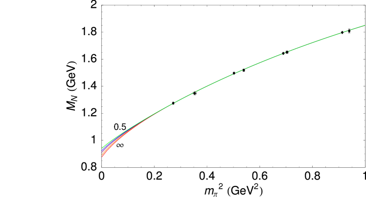
Figure 2: Dipole regulator fits to lattice data for various dipole regularization scales, $\Lambda=0.5,\ 0.8,\ 1.1,\ 2.0,\ {\rm and}\ \infty\,{\rm GeV}$, interpolating between FRR and minimal subtraction.

3 POWER-COUNTING REGIME

Because the chiral expansion of $\chi$PT is truncated with no attempt to estimate the contribution of higher-order terms, knowing the power-counting regime of a given truncation is absolutely essential to extracting correct physics from $\chi$PT. One simply obtains the wrong answer if one works outside the power-counting regime.

Now that the renormalized low-energy coefficients have been determined to the order we are working, we can use this information to estimate the power-counting regime of $\chi$PT. In the following, we quantify the power-counting regime by identifying the range of pion masses whereby the expansion is truly independent of regularization scheme and hence independent of contributions from higher-order terms in the expansion. As discussed in the introduction and in detail in Sec. 2 surrounding Eq. (13), the FRR chiral expansion is mathematically equivalent to that of $\chi$PT to the finite order one is working. In other words, these terms of the FRR expansion are independent of the regulator parameter, and any value of $\Lambda$ is allowed.

Fig. 3 illustrates the fourth-order chiral expansion for various dipole regulator parameters $\Lambda$, ranging between $0.5\,{\rm GeV}$ and $\infty$. This therefore describes a continuous transition between finite-range regularization and a minimal subtraction scheme. The renormalized coefficients and nonanalytic terms to fourth order are automatically independent of $\Lambda$. The observed changes in the curves are simply a reflection of the changes in terms beyond the order one is working. Of course, only the curves with $\Lambda\sim 1$ GeV have a residual expansion with good convergence properties allowing truncation of the expansion, without a loss of accuracy.

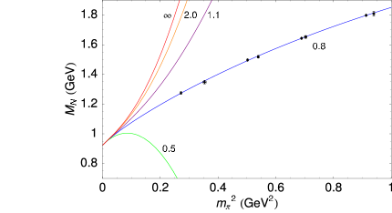
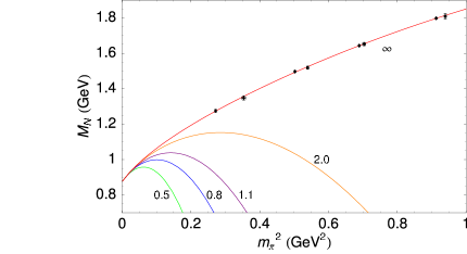
Figure 3: With the low-energy parameters $c_{0}$, $c_{2}$ and $c_{4}$ fixed to those obtained by the fit to lattice data, the chiral expansion is shown for various values of the dipole regulator scale, $\Lambda=0.5,\ 0.8,\ 1.1,\ 2.0\ {\rm and}\ \infty\,{\rm GeV}$. The left panel corresponds to the parameters $c_{i}$ determined by the $\Lambda=0.8\,{\rm GeV}$ dipole regulator fit and the right panel to those determined in the $\Lambda\to\infty$ minimal subtraction limit.

The power counting regime can be identified as the regime where the curves are independent of $\Lambda$ at some level of precision. As discussed earlier, this must be at the fraction of a percent level in order to predict the nucleon mass to an accuracy of one percent. The regime within which the curves agree within one percent is $0\leq m_{\pi}\leq 0.18\,{\rm GeV}$. This is displayed in Fig. 4, where the relative error between the two extremal regularization scales shows the sensitivity to higher orders in the chiral expansion.

Figure 4: For fixed low-energy coefficients $c_{0}$, $c_{2}$ and $c_{4}$, the relative difference in the nucleon mass expansion for two extremal regularization scales, where $\delta M_{N}=M_{N}(\Lambda=\infty)-M_{N}(\Lambda=0.5)$. The solid and dashed curve corresponds to the values of $c_{i}$ determined from the fit to lattice results with dipole of scale $\Lambda=0.8$ and $\infty\,{\rm GeV}$, respectively.

This sensitivity to higher-order terms also indicates that tolerance levels of 5% and 10% can be achieved up to pion masses of $0.25$ and $0.29\,{\rm GeV}$, respectively. These estimates of the chiral regime are similar to those reported by Beane [21], as discussed above.

The results of Fig. 4 are robust to the choice of $\Lambda$ used to obtain the leading renormalized low-energy coefficients $c_{0}$, $c_{2}$ and $c_{4}$ of the chiral expansion. Figure 3 also displays results in the extreme (and undesirable) case where the coefficients are fixed in the $\Lambda\to\infty$ (minimal subtraction) limit. The associated power-counting regime is displayed in Fig. 4 by the dashed curve, revealing a negligible difference.

4 CONCLUSIONS

As we have strictly shown, FRR is mathematically equivalent to minimal subtraction schemes such as dimensional regularization to any finite order one wishes to work. When working within the power-counting regime as defined above, the FRR and minimal-subtraction schemes are model independent.

However, when used beyond the power-counting regime, the truncated expansion of $\chi$PT fails. The signature of this failure is that the low-energy coefficients of the expansion are sacrificed to fit the lattice results, leading to values that differ from the correct values of the low-energy theory. Knowledge of the extent of the power-counting regime is as important as knowledge of the finite-order chiral expansion itself.

Methods to determine the power counting regime have been described herein. If one limits the systematic errors at the fraction of a percent level to allow a prediction of the nucleon mass at the 1% level, the power-counting regime is $0\leq m_{\pi}^{2}\leq 0.03\,{\rm GeV}^{2}$ or $0\leq m_{\pi}\leq 0.18\,{\rm GeV}$. Unfortunately, today’s lattice QCD results do not come close to this power-counting regime of fourth-order $\chi$PT. With the regime extending marginally beyond the physical pion mass, one might wonder what role, if any, traditional $\chi$PT will play in the extrapolation of lattice QCD results. The problem is exacerbated by the need to have sufficient data inside the power-counting regime to determine the fit parameters. In time, algorithms which enable dynamical-fermion simulations below $m_{\pi}=0.18\,{\rm GeV}$, are likely to permit a direct simulation at $m_{\pi}=0.140$ GeV.

In contrast, FRR schemes take on a model dependence when used outside the power-counting regime. The model-dependence associated with the shape of the regulator is at the fraction of a percent level, even over the range $0\leq m_{\pi}^{2}\leq 1.0\,{\rm GeV}^{2}$. As the expansion is truncated there is a residual dependence on the regulator parameter, $\Lambda$, which can be quantified by varying $\Lambda$ over a range where convergence of the residual expansion remains acceptable. The success of FRR is realized in that this residual degree of model-dependence in demonstrably small, such that the chiral extrapolation of modern lattice results is under control. This remarkable result is extremely important in that it is likely to provide the only reliable method to extract physical hadron properties from lattice simulation results for many years.

DBL thanks the Theory Group at Jefferson Lab for their kind hospitality during his stay while on study leave. He also thanks Tom Cohen, Stefan Scherer, Jambul Gegelia, Matthias Schindler and Vladimir Pascalutsa for interesting and helpful discussions. This work was supported by the Australian Research Council and by DOE contract DE-AC05-84ER40150, under which SURA operates Jefferson Laboratory.

References

- [1] D. B. Leinweber, D. H. Lu and A. W. Thomas, Phys. Rev. D 60, 034014 (1999) [arXiv:hep-lat/9810005]; D. B. Leinweber, A. W. Thomas, K. Tsushima and S. V. Wright, Phys. Rev. D 61 (2000) 074502 [arXiv:hep-lat/9906027]; ibid. 64 (2001) 094502 [arXiv:hep-lat/0104013]; E. J. Hackett-Jones, D. B. Leinweber and A. W. Thomas, Phys. Lett. B 494, 89 (2000) [arXiv:hep-lat/0008018]; ibid. 489, 143 (2000) [arXiv:hep-lat/0004006]; D. B. Leinweber, A. W. Thomas and R. D. Young, Phys. Rev. Lett. 86 (2001) 5011 [arXiv:hep-ph/0101211].
- [2] W. Detmold et al., Phys. Rev. Lett. 87, 172001 (2001) [arXiv:hep-lat/0103006]; W. Detmold, W. Melnitchouk and A. W. Thomas, Phys. Rev. D 66, 054501 (2002) [arXiv:hep-lat/0206001]; ibid. 68, 034025 (2003) [arXiv:hep-lat/0303015].
- [3] R. D. Young, D. B. Leinweber, A. W. Thomas and S. V. Wright, Phys. Rev. D 66 (2002) 094507 [arXiv:hep-lat/0205017].
- [4] R. D. Young, D. B. Leinweber and A. W. Thomas, Prog. Part. Nucl. Phys. 50 (2003) 399 [arXiv:hep-lat/0212031].
- [5] D. B. Leinweber, A. W. Thomas and R. D. Young, Phys. Rev. Lett. 92 (2004) 242002 [arXiv:hep-lat/0302020].
- [6] R. D. Young, D. B. Leinweber and A. W. Thomas, Phys. Rev. D 71 (2005) 014001 arXiv:hep-lat/0406001.
- [7] D. B. Leinweber et al., arXiv:hep-lat/0406002.
- [8] J. F. Donoghue, B. R. Holstein and B. Borasoy, Phys. Rev. D 59, 036002 (1999) [arXiv:hep-ph/9804281].
- [9] B. Borasoy, B. R. Holstein, R. Lewis and P. P. A. Ouimet, Phys. Rev. D 66 (2002) 094020 [arXiv:hep-ph/0210092].
- [10] V. Bernard, T. R. Hemmert and U. G. Meissner, Nucl. Phys. A 732, 149 (2004) [arXiv:hep-ph/0307115].
- [11] D. Djukanovic, M. R. Schindler, J. Gegelia and S. Scherer, arXiv:hep-ph/0407170.
- [12] V. Pascalutsa and M. Vanderhaeghen, arXiv:nucl-th/0412113.
- [13] M. Procura, T. R. Hemmert and W. Weise, Phys. Rev. D 69, 034505 (2004) [arXiv:hep-lat/0309020].
- [14] V. Pascalutsa, B. R. Holstein and M. Vanderhaeghen, Phys. Lett. B 600, 239 (2004) [arXiv:hep-ph/0407313].
- [15] A. Ali Khan et al. [QCDSF-UKQCD Collaboration], Nucl. Phys. B 689, 175 (2004) [arXiv:hep-lat/0312030].
- [16] A. Ali Khan et al. [CP-PACS Collaboration], Phys. Rev. D 65 (2002) 054505 [Erratum-ibid. D 67, 059901 (2003)] [arXiv:hep-lat/0105015].
- [17] J. A. McGovern and M. C. Birse, Phys. Lett. B 446, 300 (1999) [arXiv:hep-ph/9807384].
- [18] L. F. Li and H. Pagels, Phys. Rev. Lett. 26, 1204 (1971).
- [19] A. W. Thomas and W. Weise, The Structure of the Nucleon, Berlin, Germany: Wiley-VCH (2001).
- [20] M. K. Banerjee and J. Milana, Phys. Rev. D 54, 5804 (1996) [arXiv:hep-ph/9508340].
- [21] S. R. Beane, Nucl. Phys. B 695, 192 (2004) [arXiv:hep-lat/0403030].