BI-TP 2005/02
SWAT/05/422

Thermodynamics of Two Flavor
QCD to Sixth Order in
Quark Chemical Potential

C.R. Allton,^a M. Döring,^b S. Ejiri,^b S.J. Hands,^a O. Kaczmarek,^b F. Karsch,^b E. Laermann,^b and K. Redlich^b,c

^a Department of Physics, University of Wales Swansea, Singleton Park,

Swansea SA2 8PP, U.K.

^b Fakultät für Physik, Universität Bielefeld, D-33615 Bielefeld, Germany.

^c Institute of Theoretical Physics, University of Wroclaw,

PL-50204 Wroclaw, Poland.

ABSTRACT

We present results of a simulation of two flavor QCD on a $16^{3}\times 4$ lattice using p4-improved staggered fermions with bare quark mass $m/T=0.4$. Derivatives of the thermodynamic grand canonical partition function $Z(V,T,\mu_{u},\mu_{d})$ with respect to chemical potentials $\mu_{u,d}$ for different quark flavors are calculated up to sixth order, enabling estimates of the pressure and the quark number density as well as the chiral condensate and various susceptibilities as functions of $\mu_{q}=(\mu_{u}+\mu_{d})/2$ via Taylor series expansion. Furthermore, we analyze baryon as well as isospin fluctuations and discuss the relation between the radius of convergence of the Taylor series and the chiral critical point in the QCD phase diagram. We argue that bulk thermodynamic observables do not, at present, provide direct evidence for the existence of a chiral critical point in the QCD phase diagram. Results are compared to high temperature perturbation theory as well as a hadron resonance gas model.

PACS numbers: 12.38.Gc, 12.38.Mh

1 Introduction

The thermodynamics of strongly interacting matter has been studied extensively in lattice calculations at vanishing quark chemical potential, $\mu_{q}$ (or baryon $\mu_{B}\equiv 3\mu_{q}$) [1]. Current lattice calculations strongly suggest that the transition from the hadronic low temperature phase to the high temperature phase is a continuous, non-singular but rapid transition happening in a narrow temperature interval around the transition temperature $T_{0}\simeq 170$ MeV. Recent advances in the development of techniques for lattice calculations at non-zero quark chemical potential $\mu_{q}$ [2, 3, 4, 5, 6] have also enabled the first exploratory studies of the QCD phase diagram and bulk thermodynamics in a regime of small $\mu_{q}$, i.e. for $\mu_{q}/T\ \raise 1.29167pt\hbox{$<$\kern-7.5pt\raise-4.73611pt\hbox{$\sim$}}\ 1$ and $T\ \raise 1.29167pt\hbox{$>$\kern-7.5pt\raise-4.73611pt\hbox{$\sim$}}\ 0.8\ T_{0}$.

Guided by phenomenological models which suggest that at low temperature and non-zero quark chemical potential the low and high density regions will be separated by a first order phase transition it has been speculated [7] that a $2^{nd}$ order phase transition point, the chiral critical point, exists in the interior of the QCD phase diagram, at which the line of first order transitions ends. For smaller values of $\mu_{q}/T$ the low and high temperature regime will then be only separated by a crossover transition. The first exploratory studies at non-zero quark chemical potential indeed gave evidence for such a chiral critical point [2], although subsequent investigations made clear that at present any quantitative statement about the location [8, 9] and maybe even about the existence of such a chiral critical point is premature. The first calculations of the baryonic contribution to the pressure in strongly interacting matter [3, 10, 11, 12, 13, 14] also suggested that the transition and the thermodynamic behaviour in the high-T phase resemble the picture found previously at zero net baryon density. In this case ($\mu_{q}=0$) the transition occurs over a narrow temperature interval. Beyond a region $T\in[T_{0},1.5T_{0}]$ where there are large deviations from ideal gas behaviour, thermodynamic observables rapidly approach the high-T ideal gas limit; for instance, the pressure agrees with the Stefan-Boltzmann prediction to within $\sim 20\%$. In the low temperature hadronic phase it has been found that a hadron resonance gas model provides an astonishingly good description of basic features of the $T$ and $\mu_{q}$-dependence of thermodynamic observables [15].

Maybe one of the largest changes compared to the thermodynamics at $\mu_{q}\equiv 0$ has been observed in the temperature dependence of the quark number and isovector susceptibilities [11]. For $\mu_{q}=0$ these observables show a similar temperature dependence. They have been found to change rapidly at the transition temperature but continue to increase monotonically at larger temperatures [16, 17, 18, 19, 20]. For $\mu_{q}>0$, however, the quark number susceptibility develops a pronounced peak at the transition temperature while the isovector susceptibility continues to show a temperature dependence similar to that found at $\mu_{q}=0$. Such a behavior, indeed, is expected to occur in QCD in the vicinity of a $2^{nd}$ order phase transition point [21]. Susceptibilities thus may provide the most direct evidence for the existence of a $2^{nd}$ order phase transition in the QCD phase diagram. Finding the characteristic volume and/or quark mass dependent universal scaling behavior of susceptibilities would undoubtedly establish the existence of a chiral critical point.

In this paper we want to extend our previous study of thermodynamics at non-zero quark chemical potential [3, 11], which is based on a Taylor series expansion around $\mu_{q}=0$, to the $6^{th}$ order. Going to higher orders in the expansion is of particular importance for the analysis of higher derivatives of the density of the grand potential expressed in units of the temperature, $\Omega(V,T,\mu)\equiv(VT^{3})^{-1}\ln Z$, i.e. for an analysis of generalized susceptibilities. Accordingly our main emphasis will be to further analyze the properties of quark number and isovector susceptibilities, relate them to diagonal and non-diagonal flavor susceptibilities, calculate the chiral susceptibility and discuss to what extent the pronounced peaks found in some of these susceptibilities give evidence for the existence of a chiral critical point in the QCD phase diagram.

This paper is organized as follows. We start in the next section by summarizing basic results on QCD thermodynamics at non-zero quark chemical potential obtained in high temperature perturbation theory [22, 23] and expectations based on properties of the hadron resonance gas model at low temperature [24, 25]. In section 3 we present results on the calculation of various thermodynamic observables obtained from a Taylor expansion up to $6^{th}$ order in $\mu_{q}/T$. In section 4 we analyze the convergence properties of the Taylor series. Section 5 is devoted to a discussion of the reweighting approach to QCD thermodynamics at $\mu_{q}\neq 0$ and its comparison to the Taylor expansion approach. In section 6 we give our conclusions. An Appendix contains details on the Taylor expansion of various observables studied here.

2 Thermodynamics at low and high temperature

In this section we want to briefly discuss the density or chemical potential dependence of thermodynamic observables in the asymptotic high temperature regime as well as at low temperatures in the hadronic phase of QCD. On the former we have information from high temperature perturbation theory which recently has been extended to ${\cal O}(g^{6}\ln g)$ [23] also for non-vanishing quark chemical potentials $\mu_{f}$, $f=u,~{}d,..$, and as for $\mu_{f}\equiv 0$ [26] is thus now known to all perturbatively calculable orders. Although a comparison of the perturbative expansion with lattice calculations at $\mu_{f}=0$ suggests that quantitative agreement cannot be expected at temperatures close to the transition temperature, $T_{0}$, we can gain useful insight into the structure of the Taylor expansion used in lattice calculations to study thermodynamics at $\mu_{f}\neq 0$.

In the low temperature hadronic phase a systematic QCD based analysis is difficult and one generally has to rely on calculations within the framework of effective low energy theories or to phenomenological approaches. Here we will focus on a discussion of the properties of a hadron resonance gas model, which recently has been compared to lattice results at non-zero quark chemical potential quite successfully [15] and which also is known to describe experimental results on the chemical freeze-out of particle ratios observed in heavy ion collisions rather well [25].

2.1 High temperature perturbation theory

In the infinite temperature limit the grand potential of QCD, $\Omega(T,\mu)\equiv\ln{\cal Z}(V,T,\mu)/VT^{3}$, which is equivalent to the pressure in units of $T^{4}$, approaches that of a free quark-gluon gas (Stefan-Boltzmann (SB) gas),

$$\frac{p_{SB}}{T^{4}}=\Omega^{(0)}(T,\mu)=\frac{8\pi^{2}}{45}+\sum_{f=u,d,..}\left[\frac{7\pi^{2}}{60}+\frac{1}{2}\left(\frac{\mu_{f}}{T}\right)^{2}+\frac{1}{4\pi^{2}}\left(\frac{\mu_{f}}{T}\right)^{4}\right]\quad,$$ (2.1)

where the first term gives the contribution of the gluon sector and the sum over the fermion sector extends over $n_{f}$ different flavors. In Eq. (2.1) we only gave the result for massless quarks and gluons. Also in the following we will restrict our discussion of perturbative results to the case of QCD with massless quarks. In this section we also use $\mu$ to denote the entire set of $n_{f}$ different chemical potentials $(\mu_{u},~{}\mu_{d},...)$. We also introduce the shorthand notation $\hbox{\boldmath$\mu^{2}$\unboldmath}\equiv\sum_{f}\left(\mu_{f}/T\right)^{2}$.

The additive structure of contributions arising from gluons and the different fermion flavor sectors persists at ${\cal O}(g^{2})$. Only starting at ${\cal O}(g^{3})$ is a coupling among the different partonic sectors introduced. At this order it is induced through the non-vanishing electric (Debye) mass term $m_{E}$ [23],

$$\Omega(T,\mu)=\Omega^{(0)}(T,\mu)+g^{2}\;\Omega^{(2)}(T,\mu)+g^{3}\;\Omega^{(3)}(T,\mu)+{\cal O}(g^{4})\quad,$$ (2.2)

with

$$\Omega^{(2)}(T,\mu) = -\left(\frac{1}{6}+\frac{5n_{f}}{72}+\frac{1}{4\pi^{2}}\hbox{\boldmath$\mu^{2}$\unboldmath}+\frac{1}{8\pi^{4}}\sum_{f=u,d,..}\left(\frac{\mu_{f}}{T}\right)^{4}\right)\quad,$$

$$\Omega^{(3)}(T,\mu) = \frac{1}{6\pi}\left(\frac{m_{E}}{gT}\right)^{3}=\frac{1}{6\pi}\left(1+\frac{n_{f}}{6}+\frac{1}{2\pi^{2}}\hbox{\boldmath$\mu^{2}$\unboldmath}\right)^{3/2}\;.$$ (2.3)

The electric mass term introduces a dependence of a given quark flavor sector on changes in another sector, i.e. the quark number density in a flavor sector $\ell$,

$$\frac{n_{\ell}}{T^{3}}=\frac{\partial\Omega(T,\mu)}{\partial\mu_{\ell}/T}\quad,$$ (2.4)

depends on the other quark chemical potentials only at ${\cal O}(g^{3})$. This is also reflected in the structure of diagonal and non-diagonal susceptibilities [4, 16, 17, 18, 19, 20].

$$\frac{\chi_{ff}(T,\mu)}{T^{2}}=\frac{\partial^{2}\Omega(T,\mu)}{\partial(\mu_{f}/T)^{2}}\quad,\quad\frac{\chi_{fk}(T,\mu)}{T^{2}}=\frac{\partial^{2}\Omega(T,\mu)}{\partial(\mu_{f}/T)\partial(\mu_{k}/T)}\quad.$$ (2.5)

The diagonal susceptibilities are non-zero in the ideal gas limit and, moreover, the leading order perturbative term stays non-zero also in the limit of vanishing quark chemical potential,

$$\frac{\chi_{ff}(T,\mu)}{T^{2}} = 1+\frac{3}{\pi^{2}}\left(\frac{\mu_{f}}{T}\right)^{2}+{\cal O}(g^{2})\quad.$$ (2.6)

The non-diagonal susceptibilities, however, receive non-zero contributions only at ${\cal O}(g^{3})$. The leading perturbative contribution is positive and inversely proportional to the electric screening mass. However, it vanishes in the limit of vanishing chemical potentials. In this case the first non-zero contribution arises at ${\cal O}(g^{6}\ln 1/g)$ [22],

$$\frac{\chi_{fk}(T,\mu)}{T^{2}} = \frac{g^{3}}{2\pi^{5}}\left(1+\frac{n_{f}}{6}+\frac{1}{2\pi^{2}}\hbox{\boldmath$\mu^{2}$\unboldmath}\right)^{-1/2}\frac{\mu_{\ell}}{T}\frac{\mu_{k}}{T}+{\cal O}(g^{4})\quad,$$ (2.7)

$$\frac{\chi_{fk}(T,0)}{T^{2}} \simeq -\frac{5}{144\pi^{6}}\;g^{6}\ln 1/g\quad.$$ (2.8)

As we are going to discuss lattice calculations at non-zero chemical potential which are based on a Taylor expansion of the grand potential $\Omega$ in terms of $\mu_{f}/T$ it also is instructive to consider a Taylor expansion of the perturbative series for $\Omega$. While perturbative terms up to ${\cal O}(g^{2})$ only contribute to the series up to ${\cal O}(\mu^{4})$ higher order terms in the expansion start receiving non-vanishing contributions at ${\cal O}(g^{3})$. These again arise from the electric mass term, i.e. from an expansion of $m_{E}/gT$ in powers of $\mu^{2}$;

$$\Omega^{(3)} = \frac{1}{6\pi}\left(1+\frac{n_{f}}{6}\right)^{3/2}+\frac{1}{8\pi^{3}}\left(1+\frac{n_{f}}{6}\right)^{1/2}\hbox{\boldmath$\mu^{2}$\unboldmath}+\frac{1}{64\pi^{5}}\left(1+\frac{n_{f}}{6}\right)^{-1/2}\left(\hbox{\boldmath$\mu^{2}$\unboldmath}\right)^{2}$$ (2.9)

$$-\frac{1}{768\pi^{7}}\left(1+\frac{n_{f}}{6}\right)^{-3/2}\left(\hbox{\boldmath$\mu^{2}$\unboldmath}\right)^{3}+{\cal O}(\mu^{8})\quad.$$

Note that the expansion coefficients up to and including ${\cal O}(\mu^{4})$ are positive. Starting at ${\cal O}(\mu^{6})$ they alternate in sign. From the sign of the $\mu^{6}$-term it follows via Eq. (2.5) that the leading perturbative contribution to the expansion coefficient of diagonal as well as non-diagonal susceptibilities at ${\cal O}(\mu^{4})$ is negative, with the latter being an order of magnitude smaller.

Rather than discussing the thermodynamics of QCD at non vanishing quark chemical potential in terms of chemical potentials related to quark numbers in different flavor channels, it is convenient to introduce chemical potentials which are related to conserved quantum numbers considered at low energy, i.e. quark or baryon number and isospin. In the case of two flavor QCD, which we are going to analyze in our lattice calculations, we thus introduce also the quark chemical potential, $\mu_{q}=(\mu_{u}+\mu_{d})/2$ and the isovector chemical potential $\mu_{I}=(\mu_{u}-\mu_{d})/2$. In analogy to Eq. (2.5) we then can introduce quark number and isovector susceptibilities,

$$\frac{\chi_{q}}{T^{2}}=\frac{\partial^{2}\Omega}{\partial(\mu_{q}/T)^{2}}\equiv 2\left(\chi_{uu}+\chi_{ud}\right)\quad,\quad\frac{\chi_{I}}{T^{2}}=\frac{\partial^{2}\Omega}{\partial(\mu_{I}/T)^{2}}\equiv 2\left(\chi_{uu}-\chi_{ud}\right)\quad,$$ (2.10)

where in the second equality we have assumed degenerate $(u,d)$-quark masses.

2.2 Low temperature hadron resonance gas

The success in describing particle abundance ratios observed in heavy ion experiments at varying beam energies in terms of equilibrium properties of a hadron resonance gas model [25] begs a comparison of this model for the low temperature hadronic phase with lattice QCD calculations. Indeed this led to astonishingly good agreement [15].

In the hadron resonance gas (HRG) model it is assumed that for $T<T_{0}$ the QCD partition function can be approximated by that of a non-interacting gas of hadron resonances, either bosonic mesons or fermionic baryons. This, however, does not mean that interactions in dense hadronic matter have been ignored; in the spirit of Hagedorn’s bootstrap model [24] the inclusion of heavy resonances as stable particles also takes care of the interaction among the hadrons in the dense gas at low temperature.

The partition function of the hadron resonance gas may be split into mesonic and baryonic contributions,

$$\ln{\cal Z}_{HRG}(T,V,\mu_{q},\mu_{I})=\sum_{i\in\;mesons}\ln{\cal Z}^{M}_{m_{i}}(T,V,\mu_{q},\mu_{I})+\sum_{i\in\;baryons}\ln{\cal Z}^{B}_{m_{i}}(T,V,\mu_{q},\mu_{I})\;,$$ (2.11)

where

$$\ln{\cal Z}^{M/B}_{m_{i}}(T,V\mu_{q},\mu_{I})=\mp{V\over{2\pi^{2}}}\int_{0}^{\infty}dkk^{2}\ln(1\mp z_{i}e^{-\varepsilon_{i}/T})\quad,$$ (2.12)

with energies $\varepsilon_{i}^{2}=k^{2}+m_{i}^{2}$ and fugacities

$$z_{i}=\exp\left((3B_{i}\mu_{q}+2I_{3i}\mu_{I})/T\right)\quad.$$ (2.13)

Here $B_{i}$ is the baryon number and $I_{3i}$ denotes the third component of the isospin of the species in question. The upper sign in Eq. (2.12) refers to bosons, and the lower sign to fermions. Note that with this convention anti-particles must be counted separately in Eq. (2.11) with fugacity $z_{i}^{-1}$, and self-conjugate species such as $\pi^{0},\eta^{\prime}$ have $z=1$. If the logarithms are expanded in powers of fugacity, the integral over momenta, $k$, can be performed. This yields

$$\ln{\cal Z}^{M/B}_{m_{i}}=\frac{VTm_{i}^{2}}{2\pi^{2}}\sum_{\ell=1}^{\infty}\left\{\matrix{1\cr(-1)^{\ell+1}}\right\}\ell^{-2}K_{2}\left(\frac{\ell m_{i}}{T}\right)z_{i}^{\ell}\quad,$$ (2.14)

where the upper factor in braces applies to bosons and the lower to fermions, and $K_{2}$ is a modified Bessel function. For large argument, i.e. for $m_{i}\gg T$ the Bessel function can be approximated by $K_{2}(x)\sim\sqrt{\pi/2x}\;{\rm e}^{-x}(1+15/8x+{\cal O}(x^{-2}))$. Terms with $\ell\geq 2$ in the series given in Eq. (2.14) thus are exponentially suppressed. For temperatures and quark chemical potentials less than a typical scale of about $200~{}$MeV it generally suffices to keep the first term in the sum appearing in Eq. (2.14). The only species for which this step would need further justification is the pion; clearly for realistic pion masses more care must be taken when evaluating the sum over $\ell$. This, however, does not influence the $\mu_{q}$-dependence of the hadron resonance gas; $B_{i}=0$ for mesons and their contribution thus is independent of $\mu_{q}$. At $\mu_{I}=0$ one readily derives,

$${p(T,\mu_{q})\over T^{4}}=\frac{1}{VT^{3}}\ln{\cal Z}_{HRG}\biggr{|}_{\mu_{I}=0}\simeq G(T)+F(T)\cosh\left(\frac{3\mu_{q}}{T}\right)\quad,$$ (2.15)

with $G(T)=(VT^{3})^{-1}\sum_{i\in mesons}\ln{\cal Z}^{M}_{m_{i}}$ and $F(T)$ given by the Boltzmann approximation to the fermion partition function of baryons,

$$F(T) = {1\over\pi^{2}}\sum_{i\in\;baryons}\left({m_{i}\over T}\right)^{2}K_{2}\left({m_{i}\over T}\right)\quad.$$ (2.16)

Note that each term in the sum for $F$ now counts both baryon and anti-baryon. As the meson sector of the partition functions is independent of $\mu_{q}$ the mesonic component does not contribute to $\chi_{q}$,

$${\chi_{q}\over T^{2}}=9F(T)\cosh{{3\mu_{q}}\over T}\quad.$$ (2.17)

Similarly, at $\mu_{I}=0$ we find for the isovector susceptibility

$${\chi_{I}\over T^{2}}=G^{I}(T)+F^{I}(T)\cosh{{3\mu_{q}}\over T}$$ (2.18)

with

$$G^{I}(T) = {1\over 2\pi^{2}}\sum_{i\in\;mesons}\sum_{\ell=1}^{\infty}(2I_{3i})^{2}\left({m_{i}\over T}\right)^{2}K_{2}\left({\ell m_{i}\over T}\right)\quad,$$

$$F^{I}(T) = {1\over\pi^{2}}\sum_{i\in\;baryons}(2I_{3i})^{2}\left({m_{i}\over T}\right)^{2}K_{2}\left({m_{i}\over T}\right)\quad.$$ (2.19)

where again only in the baryon sector $\ell>1$ terms have been neglected.

The resonance gas model in the (partial) Boltzmann approximation given by Eqs. (2.15)-(2.19) leads to simple predictions for the dependence of thermodynamic observables on the quark chemical potential $\mu_{q}$. In particular, it predicts that ratios of the density dependent part of thermodynamic observables are insensitive to details of the hadronic mass spectrum. Nor do they depend explicitly on temperature, but instead only on the ratio $\mu_{q}/T$. For instance, one finds

$$\frac{p(T,\mu_{q})-p(T,0)}{\chi_{q}T^{2}}=\frac{\cosh(3\mu_{q}/T)-1}{9\cosh(3\mu_{q}/T)}\quad,\quad\frac{n_{q}}{\mu_{q}\chi_{q}}=\frac{T}{3\mu_{q}}\tanh\left(\frac{3\mu_{q}}{T}\right)\quad.$$ (2.20)

Similarly ratios of Taylor expansion coefficients of thermodynamic quantities, $X$, are temperature and spectrum independent. For an observable $X$, of generic form $X=G^{X}+F^{X}\cosh(3\mu_{q}/T)$, the expansion in $\mu_{q}/T$ is given by

$$X=\sum_{n=0}^{\infty}c_{n}^{X}(T)(\mu_{q}/T)^{n},\hskip 14.22636pt$$ (2.21)

with

$$c_{0}^{X}=G^{X}+F^{X},\hskip 14.22636ptc_{2n}^{X}=\frac{9^{n}}{(2n)!}F^{X}$$ (2.22)

and $c_{2n+1}^{X}=0$. Hence, ratios are given by

$$\frac{c_{2n+2}^{X}}{c_{2n}^{X}}=\frac{9}{(2n+2)(2n+1)}\hskip 14.22636pt{\rm for}\ n\geq 1\quad.$$ (2.23)

These ratios as well as ratios of physical observables calculated within the resonance gas approximation will be compared to corresponding lattice results in the following.

3 Taylor expansion for two flavor QCD

The basic concepts of our Taylor expansion approach to QCD thermodynamics at non-zero quark chemical potential have been introduced in [11] where observables have been analyzed up to ${\cal O}(\mu_{q}^{4})$. Here we extend the analysis up to the sixth order in $\mu_{q}/T$ with significantly improved statistics.

Our calculations have been performed for two flavor QCD on an $16^{3}\times 4$ lattice with bare quark mass $ma=0.1$ using Symanzik-improved gauge and p4-improved staggered fermion actions. These parameters are identical to those used for our analysis of thermodynamic observables at non-zero chemical potential up to ${\cal O}(\mu_{q}^{4})$ [3, 11]. The simulation uses the hybrid R molecular dynamics algorithm, and measurements were performed on equilibrated configurations separated by 5 units of molecular dynamics time $\tau$. The gauge couplings, $\beta=6/g^{2}$, used for our calculations cover the interval [3.52,4.0], which corresponds to a temperature range $T/T_{0}\in[0.76,1.98]$, where $T_{0}$ is the pseudocritical temperature at $\mu=0$ for which we use $\beta_{c}=3.65$. This value is used to define the temperature scale $T/T_{0}$. The number of configurations generated at each $\beta$-value is given in Table 3.1. The third and seventh columns give the sample sizes used in [11], where coefficients up to $n=4$ were calculated. The numbers of additional configurations generated for the present study of expansion coefficients up to $n=6$ are listed in the fourth and eighth columns. It can be seen that we have increased our statistics in the hadronic phase by a factor 4-5 and in the plasma phase by a factor 3.

For the calculation of various operator traces we use the method of noisy estimators. We generally found that expectation values involving odd derivatives of $\ln{\rm det}M$ with respect to $\mu$ are noisier and require averages over more random vectors than needed to estimate expectation values involving only even derivatives. Odd derivatives have to appear in even numbers in an expectation value in order for this to be non-zero. Such expectation values behave very much like susceptibilities and receive their largest contributions in the vicinity of $T_{0}$. Still their total contribution to the expansion of e.g. the pressure is found to be small up to ${\cal O}(\mu^{4})$. It only becomes sizeable at ${\cal O}(\mu^{6})$. For these reasons we used 100 stochastic noise vectors to estimate operator traces on each configuration for $\beta\in[3.60,3.68]$. For other $\beta$ values 50 noise vectors were found to suffice.

$\beta$	$T/T_{c}$	#(2,4)	#(2,4,6)	$\beta$	$T/T_{c}$	#(2,4)	#(2,4,6)
3.52	0.76	1000	3500	3.70	1.11	800	2000
3.55	0.81	1000	3500	3.72	1.16	500	2000
3.58	0.87	1000	3500	3.75	1.23	500	1000
3.60	0.90	1000	3800	3.80	1.36	500	1000
3.63	0.96	1000	3500	3.85	1.50	500	1000
3.65	1.00	1000	4000	3.90	1.65	500	1000
3.66	1.02	1000	4000	3.95	1.81	500	1000
3.68	1.07	800	3600	4.00	1.98	500	1000

Table 3.1: Sample size at each $\beta$ value.

3.1 Pressure, quark number density and susceptibilities

To start the discussion of lattice results on thermodynamics of two flavor QCD for small values of the quark chemical potential we will present results obtained from a Taylor expansion of the grand potential $\Omega(T,\mu_{u},\mu_{d})\equiv\Omega(T,\mu_{q}+\mu_{I},\mu_{q}-\mu_{I})$ and some of its derivatives. We will consider expansions in terms of $\mu_{q}/T$ at fixed, vanishing $\mu_{I}$. The pressure is then given by

$T/T_{c}$	$c_{2}$	$c_{4}\times 10$	$c_{6}\times 10^{2}$	$c^{I}_{2}$	$c^{I}_{4}\times 10$	$c^{I}_{6}\times 10^{2}$
0.76	0.0243(19)	0.238(61)	-1.12(121)	0.0649(6)	0.098(5)	0.23(9)
0.81	0.0450(20)	0.377(64)	1.98(141)	0.0874(8)	0.140(6)	0.44(10)
0.87	0.0735(23)	0.506(68)	1.69(155)	0.1206(11)	0.216(8)	0.60(13)
0.90	0.1015(24)	0.765(72)	2.06(159)	0.1551(14)	0.302(12)	0.83(18)
0.96	0.2160(31)	1.491(135)	4.96(260)	0.2619(21)	0.564(23)	1.47(37)
1.00	0.3501(32)	2.133(121)	-5.00(359)	0.3822(26)	0.839(28)	0.26(49)
1.02	0.4228(33)	2.258(118)	-4.49(312)	0.4501(27)	0.909(28)	0.02(44)
1.07	0.5824(23)	1.417(62)	-5.73(158)	0.5972(21)	0.741(17)	-0.75(26)
1.11	0.6581(20)	0.951(39)	-1.65(62)	0.6662(18)	0.618(11)	-0.18(10)
1.16	0.7091(15)	0.763(24)	-0.31(26)	0.7156(14)	0.564(6)	-0.03(4)
1.23	0.7517(16)	0.667(23)	-0.44(23)	0.7573(13)	0.527(5)	-0.06(3)
1.36	0.7880(11)	0.572(12)	-0.09(11)	0.7906(9)	0.495(3)	-0.03(1)
1.50	0.8059(10)	0.539(10)	-0.17(7)	0.8076(7)	0.477(2)	-0.05(1)
1.65	0.8157(8)	0.499(7)	-0.13(8)	0.8169(7)	0.461(2)	-0.05(1)
1.81	0.8203(8)	0.497(7)	-0.11(6)	0.8218(6)	0.452(1)	-0.05(1)
1.98	0.8230(7)	0.473(6)	0.03(4)	0.8250(6)	0.441(1)	-0.03(1)

Table 3.2: Taylor expansion coefficients $c_{n}(T)$ and $c^{I}_{n}(T)$.

$${p\over T^{4}}\equiv\Omega(T,\mu_{q},\mu_{q})=\sum_{n=0}^{\infty}c_{n}(T)\left({\mu_{q}\over T}\right)^{n}.$$ (3.1)

CP symmetry implies that the series is even in $\mu_{q}$, so the coefficients $c_{n}$ are non-zero only for $n$ even, and are defined as

$$c_{n}(T)={1\over n!}{{\partial^{n}\Omega}\over{{\partial(\mu_{q}/T)^{n}}}}\biggr{|}_{\mu_{q}=0}={1\over n!}{N_{\tau}^{3}\over N_{\sigma}^{3}}{{\partial^{n}\ln{\cal Z}}\over{\partial(\mu N_{\tau})^{n}}}\biggr{|}_{\mu=0}\quad,$$ (3.2)

where in the second equality we have explicitly specified that the calculations have been performed on a $N_{\sigma}^{3}\times N_{\tau}$ lattice with dimensionless quark chemical potential $\mu\equiv\mu_{q}a$. ${\cal Z}$ denotes the lattice regularized partition function for two flavor QCD. Similarly we calculate the quark number density

$$\frac{n_{q}(T,\mu_{q})}{T^{3}}=\frac{\partial\Omega(T,\mu_{q},\mu_{q})}{\partial\mu_{q}/T}=2c_{2}\left(\frac{\mu_{q}}{T}\right)+4c_{4}\left(\frac{\mu_{q}}{T}\right)^{3}+6c_{6}\left(\frac{\mu_{q}}{T}\right)^{5}+\cdots\quad,$$ (3.3)

as well as the quark and isovector susceptibilities using Eq. (2.10),

$${\chi_{q}(T,\mu_{q})\over T^{2}} = 2c_{2}+12c_{4}\left({\mu_{q}\over T}\right)^{2}+30c_{6}\left({\mu_{q}\over T}\right)^{4}+\cdots$$ (3.4)

$${\chi_{I}(T,\mu_{q})\over T^{2}} = 2c^{I}_{2}+12c^{I}_{4}\left({\mu_{q}\over T}\right)^{2}+30c^{I}_{6}\left({\mu_{q}\over T}\right)^{4}+\cdots$$ (3.5)

where

$$c^{I}_{n}={1\over n!}{\partial^{n}\;\Omega(T,\mu_{q}+\mu_{I},\mu_{q}-\mu_{I})\over{{\partial(\mu_{I}/T)^{2}}\partial(\mu_{q}/T)^{n-2}}}\biggr{|}_{\mu_{q}=0,\mu_{I}=0}\quad.$$ (3.6)

Explicit expressions for $c_{2}$, $c_{4}$, $c_{6}$ and $c^{I}_{2}$, $c^{I}_{4}$ and $c^{I}_{6}$ are given in the Appendix. Note that the expansion for the quark number susceptibility $\chi_{q}$ given in Eq. (3.4) is a derivative of the grand potential at $\mu_{I}\equiv 0$ and thus has the same radius of convergence as that of the pressure and quark number density given by Eqs. (3.1) and (3.3). The expansion coefficient $c_{2}^{I}$ also defines the first term in an expansion of the pressure at non-zero isospin. This series may have a different radius of convergence [28]; indeed, since the lightest particle carrying non-zero isospin $I_{3}$ in the hadronic phase is the pion, we might expect the expansion to break down in the chiral limit for arbitrarily small $\mu_{I}$.

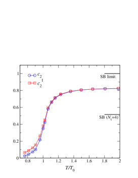
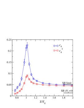
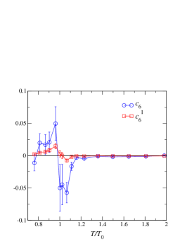
Figure 3.1: The Taylor expansion coefficients $c_{n}$ and $c^{I}_{n}$ for $n=2,4$ and 6 as functions of $T/T_{0}$.

The coefficient $c_{0}(T)$ gives the pressure in units of $T^{4}$ at vanishing baryon density and can be calculated using the integral method [29]. It is the only expansion coefficient which also requires lattice calculations at zero temperature. Higher order terms can be calculated directly from gauge field configurations generated on finite temperature lattices. They, however, require additional derivatives of $\ln\mbox{det}M$, where $M$ is the quark matrix. They are evaluated at fixed temperature, i.e. fixed gauge coupling $\beta$, by calculating combinations of traces of products of $\partial^{m}M/\partial\mu^{m}$ and $M^{-1}$ (see Appendix).

Results for the Taylor expansion coefficients are listed in Table 3.2. In Fig. (3.1) we plot $c_{n}$ and $c^{I}_{n}$ for $n=2,~{}4$ and 6 as functions of $T$. A comparison with Figs. 3 and 8 of Ref. [11] reveals the improvement in statistics of the current study. The same features are apparent: namely $c_{2}$ and $c^{I}_{2}$ both rise steeply across $T_{0}$ with $c_{2}^{I}>c_{2}$ as is obvious from the explicit expressions given for these coefficients in the appendix; they reach a plateau at approximately 80% of the value $n_{\rm f}/2$ predicted in the Stefan-Boltzmann (SB) limit, i.e. for free massless quarks; $c_{4}$ rises steeply to peak at $T\simeq T_{0}$ before approaching its SB limit value $n_{\rm f}/4\pi^{2}$ from above, whereas the peak in $c^{I}_{4}$ is much less marked.

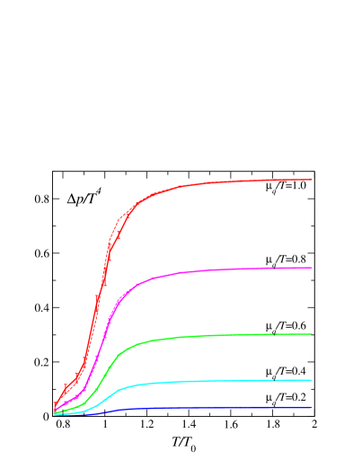
(a)

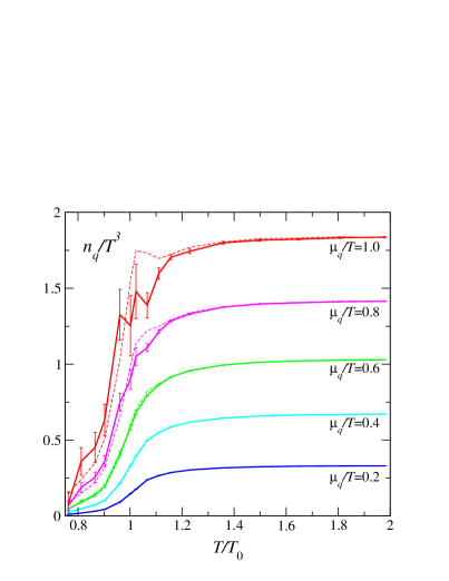
(b)

Figure 3.2: The $\mu_{q}$ dependent contribution to the pressure (left) and the quark number density (right) as functions of $T/T_{0}$ for various values of the quark chemical potential calculated from a Taylor series in $6^{th}$ order. Also shown as dashed lines are results from a $4^{th}$ order expansion in $\mu_{q}/T$.

As can be seen in Table 3.2 in the high temperature phase the $6^{th}$ order expansion coefficients generally are an order of magnitude smaller than the $4^{th}$ order coefficients. In the low temperature phase they are still a factor 3-5 smaller. As a consequence the $6^{th}$ order contributions to the pressure and quark number density are small for $\mu_{q}/T\leq 1$. This is seen in Fig. (3.2) which shows $\Delta p/T^{4}\equiv(p(T,\mu_{q})-p(T,0))/T^{4}$ and $n_{q}/T^{3}$ in the range $0\leq\mu_{q}/T\leq 1$. Here we also show as dashed lines results obtained from a Taylor expansion which includes only terms up to $4^{th}$ order in $\mu_{q}/T$. This suggests that the expansion for the pressure and quark number density is converging rapidly for $\mu_{q}/T<1$. Even for $\mu_{q}/T=1$ the differences between the $4^{th}$ and $6^{th}$-order results are small and partly influenced by statistics. We also note that in the high temperature regime, $T\raise 1.29167pt\hbox{$>$\kern-7.5pt\raise-4.73611pt\hbox{$\sim$}}1.5T_{0}$, our results are compatible with the continuum extrapolated (quenched) results obtained with an unimproved staggered fermion action [13]. This supports the expectation that deviations from the continuum limit are strongly suppressed with our improved action.

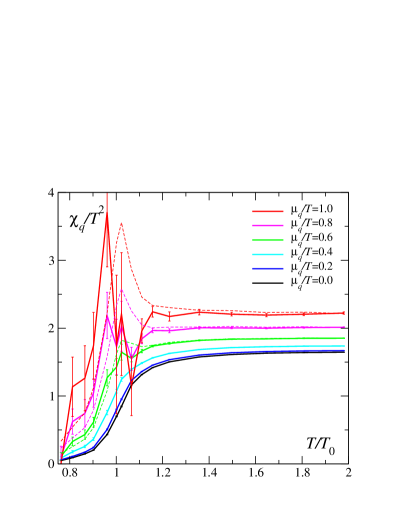
(a)

(b)

Figure 3.3: The quark number susceptibility $\chi_{q}/T^{2}$ (left) and isovector susceptibility $\chi_{I}/T^{2}$ (right) as functions of $T/T_{0}$ for various $\mu_{q}/T$ ranging from $\mu_{q}/T=0$ (lowest curve) rising in steps of 0.2 to $\mu_{q}/T=1$, calculated from a Taylor series in $6^{th}$ order. Also shown as dashed lines are results from a $4^{th}$ order expansion in $\mu_{q}/T$.

Next we turn to a discussion of quark number and isovector susceptibilities which are shown in Fig. (3.3). They have been obtained using Eqs. (3.4) and (3.5). Again we show the corresponding $4^{th}$-order results as dashed lines in these figures. These lines agree with our old results shown as Fig. 9 of [11]. The effect of the new term proportional to $c_{6}(T)$ is to shift the apparent maximum in $\chi_{q}(T)$, arising from the sharply peaked $\mu_{q}^{4}$-contribution proportional to $c_{4}(T)$, to lower temperature. This suggests that the transition temperature at non-zero $\mu_{q}$ determined from the peak position of susceptibilities indeed moves to temperatures smaller than the transition temperature $T_{0}$ determined at $\mu_{q}=0$. The figure, however, also shows that at least for $T<T_{0}$ the $6^{th}$-order contribution can be sizeable and still suffers from statistical errors. Better statistics and the contribution from higher orders in the Taylor expansion thus will be needed to get good quantitative results for susceptibilities in the hadronic phase.

There is also a pronounced dip in $\chi_{q}(T)$ for $T/T_{0}\simeq 1.05$ which, together with the increased error bars makes the presence of a peak in $\chi_{q}$ less convincing then it is without the inclusion of the $\mu_{q}^{6}$-contribution. However, the error bars also reflect the problem we have at present in determining this additional contribution with sufficient accuracy to include it in the calculation of higher order derivatives of the partition function. On the other side, Fig. (3.3) confirms that a significant peak is not present in the isovector channel. In fact, if a critical endpoint exists in the ($T,\mu$)-plane of the QCD phase diagram, this is expected to belong to the Ising universality class, implying that exactly one 3$d$ scalar degree of freedom becomes massless at this point. Since both $\bar{\psi}\psi$ and $\bar{\psi}\gamma_{0}\psi$ are isoscalar and Galilean scalars, both are candidates to interpolate this massless field, and hence we can expect divergent fluctuations in both quark number and chiral susceptibilities at this point. The latter will be discussed in section 3.3.

The difference in the temperature dependence of $\chi_{q}$ and $\chi_{I}$ also reflects the strong correlation between fluctuations in different flavor components. This will become clear from our discussion of flavor diagonal and non-diagonal susceptibilities in the next section.

3.2 Flavor diagonal and non-diagonal susceptibilities

Using the relation between quark number and isovector susceptibilities on the one hand and diagonal and non-diagonal susceptibilities on the other hand (Eq. (2.10)) we also can define expansions for the latter,

$${\chi_{uu}(T,\mu_{q})\over T^{2}}= = 2c^{uu}_{2}+12c^{uu}_{4}\left({\mu_{q}\over T}\right)^{2}+30c^{uu}_{6}\left({\mu_{q}\over T}\right)^{4}+\cdots\quad,$$ (3.7)

$${\chi_{ud}(T,\mu_{q})\over T^{2}}= = 2c^{ud}_{2}+12c^{ud}_{4}\left({\mu_{q}\over T}\right)^{2}+30c^{ud}_{6}\left({\mu_{q}\over T}\right)^{4}+\cdots\quad,$$ (3.8)

with $c_{n}^{uu}=(c_{n}+c_{n}^{I})/4$ and $c_{n}^{ud}=(c_{n}-c_{n}^{I})/4$.

As discussed in the previous section the expansion coefficients $c_{n}$ and $c^{I}_{n}$ become quite similar at high temperature. This was to be expected from the discussion of the structure of the high temperature perturbative expansion given in section 2.1 as $c_{n}$ and $c_{n}^{I}$ differ only by contributions coming from non-diagonal susceptibilities, which enter with opposite sign in these two coefficients. It thus is instructive to analyze directly the expansion coefficients of $\chi_{uu}$ and $\chi_{ud}$. These are listed in Table 3.3 and plotted in Fig. (3.4). We note that the errors on these quantities have been obtained from an independent jackknife analysis and thus are not simply obtained by adding errors for $c_{n}$ and $c_{n}^{I}$.

$T/T_{c}$	$c_{2}^{uu}\times 10^{2}$	$c_{4}^{uu}\times 10^{2}$	$c_{6}^{uu}\times 10^{2}$	$c_{2}^{ud}\times 10^{2}$	$c_{4}^{ud}\times 10^{2}$	$c_{6}^{ud}\times 10^{2}$
0.76	2.23(6)	0.84(16)	-0.22(32)	-1.015(42)	0.35(14)	-0.34(29)
0.81	3.31(6)	1.29(17)	0.60(37)	-1.060(45)	0.59(15)	0.38(33)
0.87	4.85(8)	1.81(18)	0.57(42)	-1.177(46)	0.72(16)	0.27(36)
0.90	6.41(9)	2.67(20)	0.72(44)	-1.339(45)	1.16(16)	0.31(36)
0.96	11.95(12)	5.14(39)	1.61(74)	-1.148(45)	2.32(29)	0.87(57)
1.00	18.31(14)	7.43(37)	-1.19(101)	-0.802(32)	3.23(24)	-1.31(78)
1.02	21.82(15)	7.92(36)	-1.12(88)	-0.681(27)	3.37(23)	-1.13(69)
1.07	29.49(11)	5.39(20)	-1.62(46)	-0.369(17)	1.69(11)	-1.25(33)
1.11	33.11(9)	3.92(12)	-0.46(18)	-0.205(20)	0.83(7)	-0.37(13)
1.16	35.62(7)	3.32(7)	-0.08(8)	-0.162(17)	0.50(5)	-0.07(6)
1.23	37.73(7)	2.98(7)	-0.13(6)	-0.140(22)	0.35(5)	-0.09(5)
1.36	39.47(5)	2.67(4)	-0.03(3)	-0.063(18)	0.19(3)	-0.01(2)
1.50	40.34(4)	2.54(3)	-0.06(2)	-0.043(16)	0.15(2)	-0.03(2)
1.65	40.81(4)	2.40(2)	-0.04(2)	-0.029(14)	0.10(1)	-0.02(2)
1.81	41.05(3)	2.37(2)	-0.04(2)	-0.040(14)	0.11(2)	-0.01(1)
1.98	41.20(3)	2.29(2)	-0.00(1)	-0.051(13)	0.08(1)	0.02(1)

Table 3.3: Taylor expansion coefficients $c_{n}^{uu}(T)$ and $c_{n}^{ud}(T)$.

Fig. (3.4) clearly shows that for $T>T_{0}$ the various expansion coefficients rapidly approach the corresponding ideal gas values, which is zero for all non-diagonal expansion coefficients, $c^{ud}_{n}$. In fact, as discussed in section 2.1 the latter receive contributions only at ${\cal O}(g^{6}\ln 1/g^{2})$ for $n=2$ and ${\cal O}(g^{3})$ for $n>2$. Moreover, it is interesting to note that despite the small magnitude of these contributions the leading order perturbative results correctly predict the sign of all expansion coefficients for $T>T_{0}$, i.e. $c_{2,6}^{ud}<0$, $c_{4}^{ud}>0$, and $c_{2,4}^{uu}>0$, $c_{6}^{uu}<0$. Furthermore, the order of magnitude for $c_{2}^{ud}$, i.e. $|c_{2}^{ud}|\simeq 5\cdot 10^{-4}$ at $T\simeq 2T_{0}$, agrees with the perturbative estimate [22].

Figure 3.4: The Taylor expansion coefficients $c_{n}^{uu}$ (upper row) of diagonal and $c^{ud}_{n}$ (lower row) of non-diagonal susceptibilities for $n=2,~{}4$ and 6 as functions of $T/T_{0}$.

A striking feature of the expansion coefficients $c_{n}^{uu}$ and $c_{n}^{ud}$ is that for $n>2$ they become similar in magnitude close to $T_{0}$. In fact, $c_{4}^{uu}$ and $c_{4}^{ud}$ both have pronounced peaks at $T_{0}$ with $(c_{4}^{ud}/c_{4}^{uu})_{\rm peak}\simeq 0.45$ and the expansion coefficients for $n=6$ are identical within errors. This suggests that any divergent piece in $\chi^{uu}$, which could occur when $\mu_{q}/T$ approaches the radius of convergence of the Taylor expansion, will show up with identical strength also in $\chi^{ud}$. This, in turn, implies that the singular behavior will add up constructively in the quark number susceptibility whereas it can cancel in the isovector susceptibility giving rise to finite values for $\chi_{I}$ at such a critical point. Even for smaller, non-critical values of $\mu_{q}/T$, however, the rapid rise of $c_{4}^{ud}(T)$ for $T\simeq T_{0}$ is important. It shows that non-diagonal susceptibilities will become large at non-zero chemical potential in the transition region from the low to the high temperature phase, i.e. fluctuations in different flavor channels, which are uncorrelated at high temperature, become strongly correlated in the transition region. This correlation is also reflected in the errors of the various expansion coefficients, which are of similar size for $c_{n}^{uu}$ and $c_{n}^{ud}$ but much reduced in the difference, $\chi_{I}$.

The above considerations also suggest that the electric charge susceptibility,

$$\chi_{C}=\left({2\over 3}{{\partial\;}\over{\partial\mu_{u}}}-{1\over 3}{{\partial\;}\over{\partial\mu_{d}}}\right)\left({2\over 3}{{\partial p}\over{\partial\mu_{u}}}-{1\over 3}{{\partial p}\over{\partial\mu_{d}}}\right) = \frac{1}{9}\left(4\chi_{uu}+\chi_{dd}-4\chi_{ud}\right)$$

$$= \frac{1}{4}\left(\chi_{I}+{1\over 9}\chi_{q}\right)\quad,$$ (3.9)

will be singular whenever the diagonal and non-diagonal susceptibilities are singular as the cancellation between the corresponding singular parts will be incomplete. We show the charge susceptibility in Fig. (3.5). As it is dominated by the contribution from the isovector susceptibility any possible singular contribution arising from $\chi_{q}$ will be weak. It thus may not be too surprising that a peak does not yet show up in $\chi_{C}$.

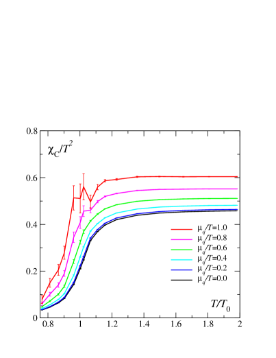
Figure 3.5: The charge susceptibility $\chi_{C}/T^{2}$ as a function of $T/T_{0}$ for various $\mu_{q}/T$ ranging from $\mu_{q}/T=0$ (lowest curve) rising in steps of 0.2 to $\mu_{q}/T=1$, calculated from a Taylor series in $6^{th}$ order.

3.3 Mass derivatives and chiral condensate

The transition between low and high temperature phases of strongly interacting matter is expected to be closely related to chiral symmetry restoration. It is therefore also of interest to analyze the dependence of the chiral condensate on the quark chemical potential. We will do so in the framework of a Taylor expansion of the grand potential,

$$\frac{\langle\bar{\psi}\psi\rangle}{T^{3}}=\left(\frac{N_{\tau}}{N_{\sigma}}\right)^{3}\frac{\partial\ln{\cal Z}}{\partial m/T}=\sum_{n=0}^{\infty}c_{n}^{\bar{\psi}\psi}(T)\left(\frac{\mu_{q}}{T}\right)^{n}\quad,$$ (3.10)

with

$$c_{n}^{\bar{\psi}\psi}=\frac{1}{n!}\left.\frac{\partial^{n}\langle\bar{\psi}\psi\rangle/T^{3}}{\partial(\mu_{q}/T)^{n}}\right|_{\mu_{q}=\mu_{I}=0}=\frac{1}{n!}\left.\frac{\partial^{n+1}\Omega}{\partial(\mu_{q}/T)^{n}\partial m/T}\right|_{\mu_{q}=\mu_{I}=0}\quad.$$ (3.11)

Here we expressed the bare lattice quark masses, $ma$, in units of the temperature by using $m/T\equiv maN_{\tau}$. For $n>0$ the expansion coefficients of the chiral condensate, are directly related to derivatives of the expansion coefficients of the grand potential $\Omega$ with respect to the quark mass, i.e. $c_{n}^{\bar{\psi}\psi}=\partial c_{n}/\partial(m/T)$. For $n=0$ this holds true up to a contribution arising from the normalization of the pressure at $(T=0,\mu_{q}=0)$. As such the coefficients $c_{n}^{\bar{\psi}\psi}$ also provide information on the quark mass dependence of other thermodynamic observables like pressure, number density or susceptibilities. For instance, the change of the quark number susceptibility with quark mass is given by

$$\frac{\partial\chi_{q}/T^{2}}{\partial m/T}=2c_{2}^{\bar{\psi}\psi}+12c_{4}^{\bar{\psi}\psi}\left({\mu_{q}\over T}\right)^{2}+{\cal O}(\mu_{q}^{4})\quad.$$ (3.12)

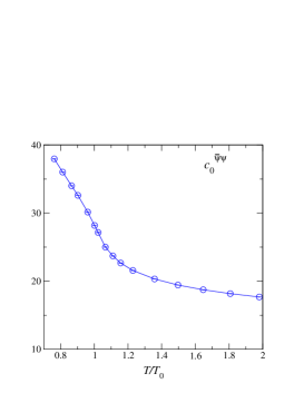
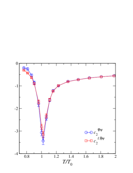
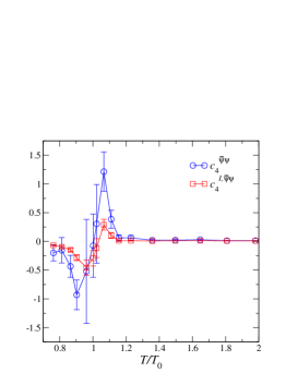
Figure 3.6: The Taylor expansion coefficients $c_{n}^{\bar{\psi}\psi}$ of the chiral condensate for $n=0,2$ and 4 as functions of $T/T_{0}$. Also shown are the coefficients $c_{n}^{I,\bar{\psi}\psi}$ for $n=0,2$ which define the quark mass derivatives of the isovector susceptibility in analogy to Eq. (3.12).

We have calculated the derivatives of $c_{n}$ with respect to the quark mass for $n=0$, 2 and 4. These derivatives are shown in Fig. (3.6) together with the corresponding derivatives for the expansion coefficients of the isovector susceptibility, which have a similar temperature dependence,

$$\frac{\partial\chi_{I}/T^{2}}{\partial m/T}=2c_{2}^{I,\bar{\psi}\psi}+12c_{4}^{I,\bar{\psi}\psi}\left({\mu_{q}\over T}\right)^{2}+{\cal O}(\mu_{q}^{4})\quad.$$ (3.13)

We note that the expansion coefficients $c_{n}^{\bar{\psi}\psi}$ are negative for $n>0$ and $T\leq 0.96T_{0}$. The chiral condensate thus will drop at fixed temperature with increasing $\mu_{q}/T$ and the chiral susceptibilities will increase in the hadronic phase with decreasing quark mass. This, together with the change of sign in $c_{4}^{\bar{\psi}\psi}$ at $T\simeq T_{0}$, will shift the transition point at non-zero $\mu_{q}/T$ to lower temperatures. In Fig. (3.7) we show the chiral condensate and the related chiral susceptibility obtained from a Taylor expansion up to and including ${\cal O}(\mu_{q}^{4})$,

$$\frac{\chi_{\bar{\psi}\psi}}{T^{2}} = \frac{N_{\tau}}{N_{\sigma}^{3}}\left(\frac{n_{\rm f}}{4}\right)^{2}\left[\left\langle\left({\rm tr}M^{-1}\right)^{2}\right\rangle-\left\langle{\rm tr}M^{-1}\right\rangle^{2}\right]$$ (3.14)

$$= c_{0}^{\chi}+c_{2}^{\chi}\left(\frac{\mu_{q}}{T}\right)^{2}+c_{4}^{\chi}\left(\frac{\mu_{q}}{T}\right)^{4}+{\cal O}\left(\left(\mu_{q}/T\right)^{6}\right)\quad.$$

Obviously $\chi_{\bar{\psi}\psi}$ develops a much more pronounced peak for $\mu_{q}/T>0$ than at vanishing chemical potential which, moreover, is shifted to smaller temperatures. However, as will become clear from the discussion in the next section the peaks found in $\chi_{\bar{\psi}\psi}$ and also in other susceptibilities have to be analyzed and interpreted carefully. They reflect the abrupt transition from the hadronic regime to the high temperature phase in which fluctuations of the chiral condensate are suppressed, but do not signal the presence of a $2^{nd}$ order phase transition unambiguously. The rapid rise of susceptibilities in the hadronic phase is strongly correlated to the increase in the pressure and is also present in a hadron gas which does not show any singular behavior at the transition temperature.

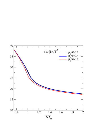
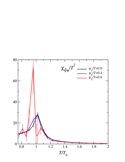
Figure 3.7: The chiral condensate $\langle\bar{\psi}\psi\rangle$ (left) and chiral susceptibility $\chi_{\bar{\psi}\psi}$ (right) as a function of $T/T_{0}$ for $\mu_{q}/T=0,~{}0.4$ and 0.8. The chiral condensate drops with increasing $\mu_{q}/T$ and the peak in $\chi_{\bar{\psi}\psi}$ becomes more pronounced.

Also the expansion of the chiral condensate and related observables are compatible with the HRG model. In fact, a comparison of the temperature dependence of $c_{n}^{\bar{\psi}\psi}$ shown in Fig. (3.6) with that of the expansion coefficients $c_{n}$ of the grand potential shown in Fig. (3.1) suggests a strong similarity between $-c_{n}^{\bar{\psi}\psi}$ and $c_{n+2}$. On the other hand, for $T<T_{0}$ the ratio $c_{4}^{\bar{\psi}\psi}/c_{2}^{\bar{\psi}\psi}$ agrees within errors with the ratio $c_{4}/c_{2}$ shown in Fig. (4.1). All this is consistent with the HRG model where the quark mass (or spectrum) dependence only enters through the functions $F(T)$ and $G(T)$ and does not modify the dependence on $\mu_{q}/T$.

4 Radius of convergence and the hadron resonance gas

So far we have not discussed the range of validity of the Taylor expansion. In general the Taylor series will only converge for $\mu_{q}/T<\rho$ (or $\mu_{q}/T\leq\rho$) where the radius of convergence, $\rho$, is determined by the zero of ${\cal Z}(T,\mu_{q},\mu_{q})$ closest to the origin of the complex $\mu_{q}$ plane. If this zero happens to lie on the real axis the radius of convergence coincides with a critical point of the QCD partition function. A sufficient condition for this is that all expansion coefficients are positive [31]. Apparently this is the case for all coefficients $c_{n}(T)$ with $T/T_{0}<0.96$ that have been calculated so far by us. Above $T_{0}$, however, we find from the calculation of $c_{6}(T)$ that the expansion coefficients do not stay strictly positive. This is in accordance with our expectation to find a chiral critical point at some temperature $T<T_{0}$.

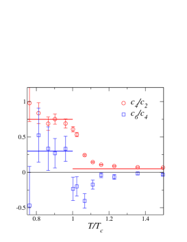
(a)

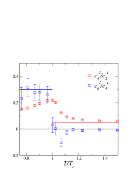
(b)

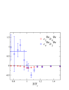
(c)

Figure 4.1: (a) The ratios $c_{4}/c_{2}$ and $c_{6}/c_{4}$, and (b) $c^{I}_{4}/c^{I}_{2}$ and $c^{I}_{6}/c^{I}_{4}$ as well as (c) $c_{2}^{\bar{\psi}\psi}/c_{0}^{\bar{\psi}\psi}$ and $c_{4}^{\bar{\psi}\psi}/c_{2}^{\bar{\psi}\psi}$ as functions of $T$. Horizontal lines indicate the HRG prediction for $T<T_{0}$, and the SB prediction for $T>T_{0}$. Note the difference in vertical scale between the plots.

The radius of convergence of the Taylor series for $\Omega(T,\mu_{q},\mu_{q})$ can be estimated by inspecting ratios of subsequent expansion coefficients,

$$\rho=\lim_{n\to\infty}\rho_{2n}\equiv\lim_{n\to\infty}\sqrt{\biggl{|}{c_{2n}\over c_{2n+2}}\biggr{|}}\quad,$$ (4.1)

where the square root arises because the Taylor expansion of the grand potential $\Omega$ is an even series in $\mu_{q}/T$. The ratios $c_{2n+2}/c_{2n}$ are shown in Fig. (4.1) together with ratios of the expansion coefficients $c_{n}^{I}$ of the isovector susceptibility and $c_{n}^{\bar{\psi}\psi}$ of the chiral condensate. It is obvious that these ratios rapidly change across $T_{0}$ and approach the value of corresponding ratios obtained in the high temperature ideal gas limit. Another remarkable feature, however, is that below $T_{0}$ the ratios involving expansion coefficients of the $\mu_{q}$-dependent parts of $\Omega$, $\chi_{I}$ and $\chi_{\bar{\psi}\psi}$ are almost temperature independent. In fact, these ratios are consistent with the corresponding ratios deduced from the grand potential of a hadron resonance gas (Eq. (2.23)), i.e. ${c_{4}/c_{2}}=c_{4}^{\bar{\psi}\psi}/c_{2}^{\bar{\psi}\psi}={3/4}$ and ${c_{6}/c_{4}}={c^{I}_{6}/c^{I}_{4}}={3/10}$. In ratios that contain the lowest order expansion coefficients, i.e. $c_{0}$, $c_{0}^{\bar{\psi}\psi}$ and $c_{2}^{I}$, the spectrum dependence does not cancel because the lowest order expansion coefficients also depend on the meson sector which is not the case for higher order coefficients. These ratios thus show a significant temperature dependence as can be seen for $c^{I}_{4}/c^{I}_{2}$ and $c_{2}^{\bar{\psi}\psi}/c_{0}^{\bar{\psi}\psi}$ shown in Fig. (4.1).

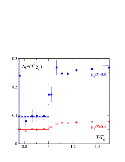
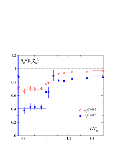
Figure 4.2: The baryonic part of the pressure divided by the quark number susceptibility, $\Delta p/\chi_{q}$ (left), and the normalized derivative of pressure with respect to quark number density, $n_{q}/\chi_{q}$ (right), as a function of $\mu_{q}/T$ for various $T/T_{0}$. Horizontal lines show the infinite temperature ideal gas values and the HRG model prediction ($T\leq T_{0}$) (solid lines) and expanded to $6^{t}h$-order in $\mu_{q}/T$ (dashed lines). The difference is visible only for $\Delta p/\chi_{q}$ at $\mu_{q}/T=0.8$.

Similar information is contained in the ratios of physical observables, e.g. the quark number density or pressure over the quark number susceptibility, introduced in Eq. (2.20). These ratios are shown in Fig. (4.2). Here $n_{q}/T^{3}$ and $\chi_{q}/T^{2}$ have been calculated using Eqs. (3.3) and (3.4) up to ${\cal O}(\mu_{q}^{6})$. The ratio, $n_{q}/\chi_{q}=(\partial p/\partial\mu_{q})/(\partial n_{q}/\partial\mu_{q})=\partial p/\partial n_{q}$ is related to the isothermal compressibility, $\kappa_{T}=\chi_{q}/n_{q}^{2}$ which diverges at a $2^{nd}$ order phase transition point, i.e. at a point at which $\partial p/\partial n_{q}=0$, the number of particles is unstable under small changes in the pressure (mechanical instability) and large density fluctuations occur. This instability leads to a divergence in the quark number susceptibility [21]. A $2^{nd}$ order phase transition is thus expected to be signalled by a zero in both ratios shown in Fig. (4.2). On the other hand, for $\mu_{I}=0$ these ratios are expected to be constant in an ideal quark-gluon plasma as well as in a hadron resonance gas,

$$\frac{n_{q}^{SB}}{\mu_{q}\chi_{q}^{SB}}=\frac{1+\frac{1}{\pi^{2}}\left(\frac{\mu_{q}}{T}\right)^{2}}{1+\frac{3}{\pi^{2}}\left(\frac{\mu_{q}}{T}\right)^{2}}\quad,\quad\frac{n_{q}^{HRG}}{\mu_{q}\chi_{q}^{HRG}}=\frac{T}{3\mu_{q}}\tanh\left(\frac{3\mu_{q}}{T}\right)\quad.$$ (4.2)

The corresponding values are indicated in Fig. (4.2) by horizontal lines.

As far as the determination of a possible $2^{nd}$ order critical point at non-vanishing quark chemical potential (chiral critical point) is concerned Fig. (4.1) and Fig. (4.2) contain identical information. For $T\leq 0.96T_{0}$ bulk thermodynamic observables agree with predictions based on an HRG model, which in itself does not show any critical behavior as function of $\mu_{q}/T$ at fixed $T$. In particular, there is no hint for a dip in $\Delta p/\chi_{q}$ or $n_{q}/\chi_{q}$ which could signal the presence of a second order transition point. The same observation, albeit with larger statistical errors, holds for ratios involving the chiral susceptibility $\chi_{\bar{\psi}\psi}$. Nonetheless, all these quantities change rapidly in the transition from the low temperature to the high temperature regime and, moreover, at $T=T_{0}$ the $6^{th}$ order expansion coefficients clearly cannot be described within the HRG model. Due to the good agreement with the HRG model and its Taylor expansion at lower temperature we cannot, however, present an upper limit for the radius of convergence below $T_{0}$; the ratios shown in Fig. (4.1) suggest that a lower limit is given by $(\mu_{q}/T)_{c}\raise 1.29167pt\hbox{$>$\kern-7.5pt\raise-4.73611pt\hbox{$\sim$}}1$. Also from the analysis of the temperature dependence of bulk thermodynamic observables we get, at present, no unambiguous evidence for the existence of a phase transition. At present, therefore, we cannot rule out that in the temperature range covered by our analysis ($T\raise 1.29167pt\hbox{$>$\kern-7.5pt\raise-4.73611pt\hbox{$\sim$}}0.8T_{0}$) the transition to the high temperature phase is a rapid crossover transition rather than a phase transition. This situation then would be similar to that at $\mu_{q}=0$. In order to exclude this possibility we would need, in the future: to consider even higher orders in the Taylor series; to scan in more detail the small temperature interval $[0.95T_{0},T_{0}]$; and to explore systematically the quark mass and volume dependence of our results. These issues are partially addressed already in the next section where we discuss the use of reweighting techniques to calculate some thermodynamic observables and compare results obtained within this approach with results from the Taylor expansion.

The good agreement found here for different ratios of Taylor expansion coefficients calculated on the lattice and within the HRG model suggests that we may use this information for a more detailed analysis of the composition of hadronic matter at temperatures below $T_{0}$. In Ref. [15] also the temperature dependence of thermodynamic observables like the pressure or the quark number susceptibility have been compared to the HRG model. In order to do so the hadron spectrum has been adjusted to the conditions realized in the lattice calculations, i.e. all masses have been shifted to larger values as the lattice calculations have been performed with unphysically large quark masses. This approach can also be turned around. The HRG model for $T<T_{0}$ can be used as an ansatz to determine the contributions of the mesonic and baryonic parts of the spectrum without making assumptions on the distortion of the spectrum due to the unphysical quark mass values.

As outlined in section 2, within the Boltzmann approximation the HRG model yields a simple dependence of the pressure on the quark chemical potential. The relation given in Eq. (2.15) can easily be extended to also include a non-vanishing isovector chemical potential. Neglecting the mass difference among isospin partners the pressure can be written as,

$$\frac{p(T,\mu_{q},\mu_{I})}{T^{4}} \simeq G^{(1)}(T)+G^{(3)}(T)\frac{1}{3}\left(2\cosh\left(\frac{2\mu_{I}}{T}\right)+1\right)$$

$$+F^{(2)}(T)\cosh\left(\frac{3\mu_{q}}{T}\right)\cosh\left(\frac{\mu_{I}}{T}\right)$$

$$+F^{(4)}(T)\frac{1}{2}\cosh\left(\frac{3\mu_{q}}{T}\right)\left[\cosh\left(\frac{\mu_{I}}{T}\right)+\cosh\left(\frac{3\mu_{I}}{T}\right)\right]~{}~{},$$

where $G^{(1)},G^{(3)},F^{(2)}$ and $F^{(4)}$ are the contributions to the pressure at $\mu_{q}=\mu_{I}=0$ arising from isosinglet mesons $(\eta,\ldots,~{}[B_{i}=0,I_{3i}=0])$, isotriplet mesons $(\pi,\ldots,~{}[B_{i}=0,I_{3i}=\{0,\pm 1\}])$, isodoublet baryons $(n,p,\ldots,~{}[B_{i}=\pm 1,I_{3i}=\{\pm 1/2\}])$ and isoquartet baryons $(\Delta,\ldots,~{}[B_{i}=\pm 1,I_{3i}=\{\pm 1/2,\pm 3/2\}])$, respectively. These functions contain all the information on the hadron spectrum in different quantum number channels. Performing the Taylor expansion of the pressure as well as quark number and isovector susceptibilities allows to relate these functions to combinations of the various Taylor expansion coefficients. This way one finds

$$G^{(3)}(T)=\frac{3}{4}c_{2}^{I}-c_{4}^{I},\hskip 22.76219ptF^{(2)}(T)=\frac{5}{18}c_{2}-\frac{2}{3}c_{4}^{I},\hskip 22.76219ptF^{(4)}(T)=-\frac{1}{18}c_{2}+\frac{2}{3}c_{4}^{I}~{}~{}.$$ (4.4)

The various contributions to the pressure are shown in Fig. (4.3)a for $\mu_{q}=0$. With increasing quark chemical potential the relative weight of hadrons in different quantum number channels changes. As expected the baryonic component becomes more important with increasing $\mu_{q}$ (Fig. (4.3)b and c). We find that for $\mu_{q}/T\raise 1.29167pt\hbox{$>$\kern-7.5pt\raise-4.73611pt\hbox{$\sim$}}0.6$ the baryonic sector gives the dominant contribution.

(a)

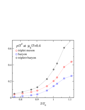
(b)

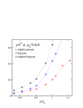
(c)

Figure 4.3: Contribution of different hadronic channels to the total pressure $p/T^{4}$ obtained by using the HRG ansatz. Shown are results for (a) $\mu_{q}/T=0$, (b) $\mu_{q}/T=0.4$ and (c) $\mu_{q}/T=0.8$.

5 Reweighting Approach

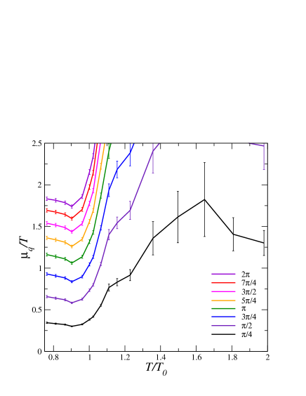
Figure 5.1: Contour plot of the variance of the phase of the quark determinant, $\sigma(\theta)$ calculated for $\theta^{(3)}$ in the $(T/T_{0},\mu_{q}/T)$ plane. Contour lines for $\sigma(\theta^{(3)})$ are given in steps of $\pi/4$ ranging from $\pi/4$ (lowest curve) to $2\pi$.

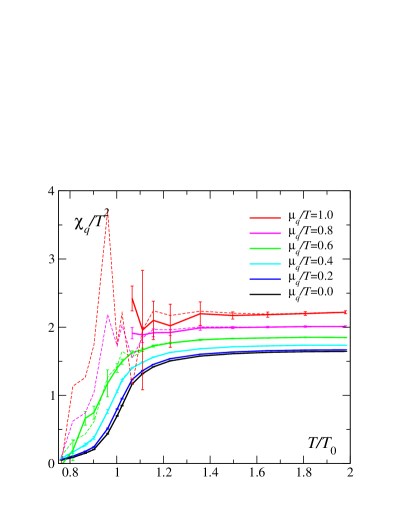
(a)

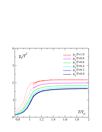
(b)

Figure 5.2: Susceptibilities $\chi_{q}/T^{2}$ (left) and $\chi_{I}/T^{2}$ (right) for various $\mu_{q}/T$ ranging from $\mu_{q}/T=0$ (lowest curve) rising in steps of 0.2 to $\mu_{q}/T=1$. Results are obtained by a combination of reweighting (solid lines and data points) and from a $6^{th}$-order Taylor expansion (dashed lines).

An alternative to a strict Taylor expansion of thermodynamic observables in terms of $\mu_{q}/T$ is the reweighting approach. Here the dependence of the grand potential on the quark chemical potential is included in the calculation of observables, $X$, by shifting the $\mu_{q}$-dependent piece of the QCD action into the calculation of expectation values rather than taking it into account in the statistical weights used for the generation of gauge field configurations. This reweighting approach has been used to analyze the thermodynamics of QCD at non-zero chemical potential [10, 12]. Within this approach thermodynamic observables $X(\beta,\mu)$ are estimated via the expression

$$\langle X\rangle_{(\beta,\mu)}={{\langle X\;e^{{n_{\rm f}\over 4}\Delta\ln{\rm det}M}e^{-\Delta S_{g}}\rangle_{(\beta_{0},0)}}\over{\langle e^{{n_{\rm f}\over 4}\Delta\ln{\rm det}M}e^{-\Delta S_{g}}\rangle_{(\beta_{0},0)}}}\quad,$$ (5.1)

where $\Delta\ln\mbox{det}M\equiv\ln{\rm det}M(\mu)-\ln{\rm det}M(0)$ and $\Delta S_{g}\equiv S_{g}(\beta)-S_{g}(\beta_{0})$ is the difference of the gluonic part of the QCD action. The expectation values on the RHS of Eq. (5.1) are obtained in simulations at $(\beta_{0},0)$. In [3] we implemented a version of Eq. (5.1) in which the reweighting factor $\Delta\ln{\rm det}M$ as well as the operator $X$ itself have been replaced by a Taylor series about $\mu=0$. The advantage over an exact evaluation of $\mbox{det}M$ [2] clearly is that the required expressions are calculable with relatively little computational effort even on large lattices. In our initial study we performed the expansion consistently up to and including ${\cal O}(\mu^{2})$. Here we extend this analysis by expanding $\ln\mbox{det}M$ up to and including terms of ${\cal O}(\mu^{6})$. Unlike the direct evaluation of thermodynamic observables in terms of a Taylor expansion up to a certain order the reweighting approach with a Taylor expanded weight factor also includes effects of higher orders in $\mu_{q}/T$ which are partially resummed in the exponentiated observables $\exp\{{n_{\rm f}\over 4}\Delta\ln{\rm det}M\}$.

The effectiveness of any reweighting approach strongly depends on the overlap between the ensemble simulated at $(\beta_{0},\mu_{0}=0)$ and that corresponding to the true equilibrium state at $(\beta,\mu)$ which one wants to analyze. This can be judged by inspecting the average phase factor of the complex valued quark determinant, $\langle e^{i\theta}\rangle_{(\beta_{0},0)}$, where the quark determinant is written as $\mbox{det}M=|\mbox{det}M|e^{i\theta}$. Reweighting loses its reliability once $\langle e^{i\theta}\rangle\ll 1$ as both expectation values appearing in the numerator and denominator of Eq. (5.1) then become difficult to control [32]. In our approach we estimate the phase factor via the variance of the phase $\theta$, $\sigma(\theta)=\sqrt{\langle\theta^{2}\rangle-\langle\theta\rangle^{2}}$, where we approximate the phase by its Taylor expansion up to ${\cal O}(\mu^{2n-1})$,

$$\theta^{(n)}={{n_{\rm f}\over 4}}\mbox{Im}\sum_{j=1}^{n}{\mu^{2j-1}\over{(2j-1)!}}{{\partial^{2j-1}\ln\mbox{det}M}\over{\partial\mu^{2j-1}}}\quad.$$ (5.2)

As discussed and shown in Fig. 6 of [32], the value of $\mu_{q}/T$ for which the standard deviation of $\theta^{(n)}$ exceeds $\pi/2$ is a reasonable criterion for judging the applicability of reweighting in our simulated systems. In Fig. (5.1) we show contour lines for the variance of $\theta^{(3)}$. All contour lines drop dramatically in the vicinity of $T_{0}$; the contour corresponding to $\sigma(\theta^{(3)})=\pi/2$ yields $\mu_{q}/T\approx 1.5$ at $T\simeq 1.2T_{0}$ and reaches a minimum value of about $0.6$ at $T\simeq 0.9T_{0}$. Reweighting is thus much easier to control in the high temperature phase than in the hadronic phase.

In Fig. (5.2) we plot quark number and isovector susceptibilities for various $\mu_{q}/T$ calculated by using reweighting where possible. The operators needed for the susceptibilities are calculated with an error of $O(\mu^{6})$, the reweighting factor $\Delta\ln\mbox{det}M$ with error $O(\mu^{8})$. Dashed lines show a comparison with the results obtained from direct Taylor expansion of the susceptibilities up to and including ${\cal O}(\mu_{q}^{4}$) (see Fig. (3.3)).

As anticipated above, for $T\raise 1.29167pt\hbox{$<$\kern-7.5pt\raise-4.73611pt\hbox{$\sim$}}T_{0}$ reweighting becomes difficult to control for $\mu_{q}/T>0.6$. However, where reweighting appears to be statistically under control, it agrees well with the direct Taylor expansion and even shows similar features in the statistical errors; i.e. the signal is much noisier in the vicinity of $T_{0}$ for $\chi_{q}$ than for $\chi_{I}$.

6 Conclusions

We have extended our analysis of the thermodynamics of two flavor QCD at non-zero quark chemical potential to the $6^{th}$ order in a Taylor expansion around $\mu_{q}/T=0$. We find clear evidence for a rapid transition from a low temperature hadronic phase to a high temperature quark-gluon plasma phase which is signalled by large fluctuations in the quark number density and the chiral condensate. The transition temperature shifts to smaller values with increasing quark chemical potential. Above $T_{0}$ the Taylor expansion coefficients and bulk thermodynamic observables agree with qualitative features of the perturbative high temperature expansion and approach the ideal gas limit to within $\sim 20\%$ for $T\raise 1.29167pt\hbox{$>$\kern-7.5pt\raise-4.73611pt\hbox{$\sim$}}1.5T_{0}$. Thermodynamics in the low temperature phase agrees well with predictions based on a hadron resonance gas for temperatures $T\raise 1.29167pt\hbox{$<$\kern-7.5pt\raise-4.73611pt\hbox{$\sim$}}0.96T_{0}$ and $\mu_{q}/T\raise 1.29167pt\hbox{$<$\kern-7.5pt\raise-4.73611pt\hbox{$\sim$}}1$.

From the analysis of bulk thermodynamic observables alone we cannot provide strong evidence for the existence of a $2^{nd}$ order phase transition point in the QCD phase diagram. At present we cannot rule out the transition being a rapid crossover in the entire parameter space covered by our analysis. In particular, we have shown that large fluctuations in the quark number and the chiral condensate are consistent with expectations based on a hadron resonance gas. The current estimates on the radius of convergence of the Taylor expansion favor a critical value of the quark chemical potential close to $\mu_{q}\approx T_{0}$. The good agreement of the expansion coefficients with those of a hadron gas, however, prohibit any firm conclusion on the location and even on the existence of the chiral critical point.

Likewise, we cannot rule out that a $2^{nd}$ order transition occurs at temperatures closer to $T_{0}$ than the largest value in the hadronic phase, $T=0.96T_{0}$ which we have analyzed here. In order to improve on the current analysis it would be important to perform calculations at smaller quark masses in a narrower temperature interval around $T_{0}$. An improvement over the current statistical errors on the $6^{th}$ order coefficient as well as the analysis of higher order expansion coefficients with high statistics is needed.

Appendix A Appendix: Taylor expansion coefficients

In this appendix, we derive some equations which are used in the calculation of the various thermodynamic quantities and expansion coefficients of the Taylor series presented in this study. The partition function is given by

$${\cal Z}=\int{\cal D}U(\det M)^{n_{\rm f}/4}e^{-S_{g}}\quad,$$ (A.1)

with $U\in SU(3)$. The expectation value of a physical quantity, $\left\langle{\cal O}\right\rangle$ is then obtained as

$$\left\langle{\cal O}\right\rangle = \frac{1}{\cal Z}\int{\cal D}U{\cal O}(\det M)^{n_{\rm f}/4}e^{-S_{g}}\quad,$$ (A.2)

and its derivatives with respect to quark chemical potential and quark mass are given by,

$$\frac{\partial\langle{\cal O}\rangle}{\partial\mu} = \left\langle\frac{\partial{\cal O}}{\partial\mu}\right\rangle+\frac{n_{\rm f}}{4}\left(\left\langle{\cal O}\;\frac{\partial(\ln\det M)}{\partial\mu}\right\rangle-\left\langle{\cal O}\right\rangle\left\langle\frac{\partial(\ln\det M)}{\partial\mu}\right\rangle\right)\quad,$$ (A.3)

$$\frac{\partial\langle{\cal O}\rangle}{\partial m} = \left\langle\frac{\partial{\cal O}}{\partial m}\right\rangle+\frac{n_{\rm f}}{4}\left(\left\langle{\cal O}\;\frac{\partial(\ln\det M)}{\partial m}\right\rangle-\left\langle{\cal O}\right\rangle\left\langle\frac{\partial(\ln\det M)}{\partial m}\right\rangle\right)$$ (A.4)

$$= \left\langle\frac{\partial{\cal O}}{\partial m}\right\rangle+\frac{n_{\rm f}}{4}\left(\left\langle{\cal O}\;{\rm tr}M^{-1}\right\rangle-\left\langle{\cal O}\right\rangle\left\langle{\rm tr}M^{-1}\right\rangle\right)\quad.$$

Here we use $m$ as the dimensionless quark mass value instead of $ma$, and also $\mu=\mu_{q}a$ for the dimensionless quark chemical potential. The temperature is $T=(N_{\tau}a)^{-1}$ and the volume is $V=(N_{\sigma}a)^{3}$. Moreover, we introduce for simplification,

$${\cal C}_{n}=\frac{n_{\rm f}}{4}\frac{\partial^{n}{\rm tr}M^{-1}}{\partial\mu^{n}}=\frac{n_{\rm f}}{4}\frac{\partial^{n+1}\ln\det M}{\partial\mu^{n}\partial m}\quad,\quad{\cal D}_{n}=\frac{n_{\rm f}}{4}\frac{\partial^{n}\ln\det M}{\partial\mu^{n}}\quad.$$ (A.5)

All Taylor expansion coefficients used in this paper can be expressed in terms of expectation values of certain combinations of ${\cal C}_{n}$ and ${\cal D}_{n}$. The required derivatives of $\ln\det M$ and ${\rm tr}M^{-1}$ are explicitly given in the following.

Derivatives of $\ln\det M$:

$$\frac{\partial\ln\det M}{\partial\mu} = {\rm tr}\left(M^{-1}\frac{\partial M}{\partial\mu}\right),$$ (A.6)

$$\frac{\partial^{2}\ln\det M}{\partial\mu^{2}} = {\rm tr}\left(M^{-1}\frac{\partial^{2}M}{\partial\mu^{2}}\right)-{\rm tr}\left(M^{-1}\frac{\partial M}{\partial\mu}M^{-1}\frac{\partial M}{\partial\mu}\right),$$ (A.7)

$$\frac{\partial^{3}\ln\det M}{\partial\mu^{3}} = {\rm tr}\left(M^{-1}\frac{\partial^{3}M}{\partial\mu^{3}}\right)-3{\rm tr}\left(M^{-1}\frac{\partial M}{\partial\mu}M^{-1}\frac{\partial^{2}M}{\partial\mu^{2}}\right)$$ (A.8)

$$+2{\rm tr}\left(M^{-1}\frac{\partial M}{\partial\mu}M^{-1}\frac{\partial M}{\partial\mu}M^{-1}\frac{\partial M}{\partial\mu}\right),$$

$$\frac{\partial^{4}\ln\det M}{\partial\mu^{4}} = {\rm tr}\left(M^{-1}\frac{\partial^{4}M}{\partial\mu^{4}}\right)-4{\rm tr}\left(M^{-1}\frac{\partial M}{\partial\mu}M^{-1}\frac{\partial^{3}M}{\partial\mu^{3}}\right)$$ (A.9)

$$-3{\rm tr}\left(M^{-1}\frac{\partial^{2}M}{\partial\mu^{2}}M^{-1}\frac{\partial^{2}M}{\partial\mu^{2}}\right)+12{\rm tr}\left(M^{-1}\frac{\partial M}{\partial\mu}M^{-1}\frac{\partial M}{\partial\mu}M^{-1}\frac{\partial^{2}M}{\partial\mu^{2}}\right)$$

$$-6{\rm tr}\left(M^{-1}\frac{\partial M}{\partial\mu}M^{-1}\frac{\partial M}{\partial\mu}M^{-1}\frac{\partial M}{\partial\mu}M^{-1}\frac{\partial M}{\partial\mu}\right),$$

$$\frac{\partial^{5}\ln\det M}{\partial\mu^{5}} = {\rm tr}\left(M^{-1}\frac{\partial^{5}M}{\partial\mu^{5}}\right)-5{\rm tr}\left(M^{-1}\frac{\partial M}{\partial\mu}M^{-1}\frac{\partial^{4}M}{\partial\mu^{4}}\right)$$ (A.10)

$$-10{\rm tr}\left(M^{-1}\frac{\partial^{2}M}{\partial\mu^{2}}M^{-1}\frac{\partial^{3}M}{\partial\mu^{3}}\right)+20{\rm tr}\left(M^{-1}\frac{\partial M}{\partial\mu}M^{-1}\frac{\partial M}{\partial\mu}M^{-1}\frac{\partial^{3}M}{\partial\mu^{3}}\right)$$

$$+30{\rm tr}\left(M^{-1}\frac{\partial M}{\partial\mu}M^{-1}\frac{\partial^{2}M}{\partial\mu^{2}}M^{-1}\frac{\partial^{2}M}{\partial\mu^{2}}\right)$$

$$-60{\rm tr}\left(M^{-1}\frac{\partial M}{\partial\mu}M^{-1}\frac{\partial M}{\partial\mu}M^{-1}\frac{\partial M}{\partial\mu}M^{-1}\frac{\partial^{2}M}{\partial\mu^{2}}\right)$$

$$+24{\rm tr}\left(M^{-1}\frac{\partial M}{\partial\mu}M^{-1}\frac{\partial M}{\partial\mu}M^{-1}\frac{\partial M}{\partial\mu}M^{-1}\frac{\partial M}{\partial\mu}M^{-1}\frac{\partial M}{\partial\mu}\right),$$

$$\frac{\partial^{6}\ln\det M}{\partial\mu^{6}} = {\rm tr}\left(M^{-1}\frac{\partial^{6}M}{\partial\mu^{6}}\right)-6{\rm tr}\left(M^{-1}\frac{\partial M}{\partial\mu}M^{-1}\frac{\partial^{5}M}{\partial\mu^{5}}\right)$$ (A.11)

$$-15{\rm tr}\left(M^{-1}\frac{\partial^{2}M}{\partial\mu^{2}}M^{-1}\frac{\partial^{4}M}{\partial\mu^{4}}\right)-10{\rm tr}\left(M^{-1}\frac{\partial^{3}M}{\partial\mu^{3}}M^{-1}\frac{\partial^{3}M}{\partial\mu^{3}}\right)$$

$$+30{\rm tr}\left(M^{-1}\frac{\partial M}{\partial\mu}M^{-1}\frac{\partial M}{\partial\mu}M^{-1}\frac{\partial^{4}M}{\partial\mu^{4}}\right)+60{\rm tr}\left(M^{-1}\frac{\partial M}{\partial\mu}M^{-1}\frac{\partial^{2}M}{\partial\mu^{2}}M^{-1}\frac{\partial^{3}M}{\partial\mu^{3}}\right)$$

$$+60{\rm tr}\left(M^{-1}\frac{\partial^{2}M}{\partial\mu^{2}}M^{-1}\frac{\partial M}{\partial\mu}M^{-1}\frac{\partial^{3}M}{\partial\mu^{3}}\right)+30{\rm tr}\left(M^{-1}\frac{\partial^{2}M}{\partial\mu^{2}}M^{-1}\frac{\partial^{2}M}{\partial\mu^{2}}M^{-1}\frac{\partial^{2}M}{\partial\mu^{2}}\right)$$

$$-120{\rm tr}\left(M^{-1}\frac{\partial M}{\partial\mu}M^{-1}\frac{\partial M}{\partial\mu}M^{-1}\frac{\partial M}{\partial\mu}M^{-1}\frac{\partial^{3}M}{\partial\mu^{3}}\right)$$

$$-180{\rm tr}\left(M^{-1}\frac{\partial M}{\partial\mu}M^{-1}\frac{\partial M}{\partial\mu}M^{-1}\frac{\partial^{2}M}{\partial\mu^{2}}M^{-1}\frac{\partial^{2}M}{\partial\mu^{2}}\right)$$

$$-90{\rm tr}\left(M^{-1}\frac{\partial M}{\partial\mu}M^{-1}\frac{\partial^{2}M}{\partial\mu^{2}}M^{-1}\frac{\partial M}{\partial\mu}M^{-1}\frac{\partial^{2}M}{\partial\mu^{2}}\right)$$

$$+360{\rm tr}\left(M^{-1}\frac{\partial M}{\partial\mu}M^{-1}\frac{\partial M}{\partial\mu}M^{-1}\frac{\partial M}{\partial\mu}M^{-1}\frac{\partial M}{\partial\mu}M^{-1}\frac{\partial^{2}M}{\partial\mu^{2}}\right)$$

$$-120{\rm tr}\left(M^{-1}\frac{\partial M}{\partial\mu}M^{-1}\frac{\partial M}{\partial\mu}M^{-1}\frac{\partial M}{\partial\mu}M^{-1}\frac{\partial M}{\partial\mu}M^{-1}\frac{\partial M}{\partial\mu}M^{-1}\frac{\partial M}{\partial\mu}\right).$$

Derivatives of ${\rm tr}M^{-1}$:

$$\frac{\partial{\rm tr}M^{-1}}{\partial\mu} = -{\rm tr}\left(M^{-1}\frac{\partial M}{\partial\mu}M^{-1}\right)$$ (A.12)

$$\frac{\partial^{2}{\rm tr}M^{-1}}{\partial\mu^{2}} = -{\rm tr}\left(M^{-1}\frac{\partial^{2}M}{\partial\mu^{2}}M^{-1}\right)+2{\rm tr}\left(M^{-1}\frac{\partial M}{\partial\mu}M^{-1}\frac{\partial M}{\partial\mu}M^{-1}\right)$$ (A.13)

$$\frac{\partial^{3}{\rm tr}M^{-1}}{\partial\mu^{3}} = -{\rm tr}\left(M^{-1}\frac{\partial^{3}M}{\partial\mu^{3}}M^{-1}\right)+3{\rm tr}\left(M^{-1}\frac{\partial^{2}M}{\partial\mu^{2}}M^{-1}\frac{\partial M}{\partial\mu}M^{-1}\right)$$

$$+3{\rm tr}\left(M^{-1}\frac{\partial M}{\partial\mu}M^{-1}\frac{\partial^{2}M}{\partial\mu^{2}}M^{-1}\right)-6{\rm tr}\left(M^{-1}\frac{\partial M}{\partial\mu}M^{-1}\frac{\partial M}{\partial\mu}M^{-1}\frac{\partial M}{\partial\mu}M^{-1}\right)$$

$$\frac{\partial^{4}{\rm tr}M^{-1}}{\partial\mu^{4}} = -{\rm tr}\left(M^{-1}\frac{\partial^{4}M}{\partial\mu^{4}}M^{-1}\right)+4{\rm tr}\left(M^{-1}\frac{\partial^{3}M}{\partial\mu^{3}}M^{-1}\frac{\partial M}{\partial\mu}M^{-1}\right)$$

$$+6{\rm tr}\left(M^{-1}\frac{\partial^{2}M}{\partial\mu^{2}}M^{-1}\frac{\partial^{2}M}{\partial\mu^{2}}M^{-1}\right)+4{\rm tr}\left(M^{-1}\frac{\partial M}{\partial\mu}M^{-1}\frac{\partial^{3}M}{\partial\mu^{3}}M^{-1}\right)$$

$$-12{\rm tr}\left(M^{-1}\frac{\partial^{2}M}{\partial\mu^{2}}M^{-1}\frac{\partial M}{\partial\mu}M^{-1}\frac{\partial M}{\partial\mu}M^{-1}\right)$$

$$-12{\rm tr}\left(M^{-1}\frac{\partial M}{\partial\mu}M^{-1}\frac{\partial^{2}M}{\partial\mu^{2}}M^{-1}\frac{\partial M}{\partial\mu}M^{-1}\right)$$

$$-12{\rm tr}\left(M^{-1}\frac{\partial M}{\partial\mu}M^{-1}\frac{\partial M}{\partial\mu}M^{-1}\frac{\partial^{2}M}{\partial\mu^{2}}M^{-1}\right)$$

$$+24{\rm tr}\left(M^{-1}\frac{\partial M}{\partial\mu}M^{-1}\frac{\partial M}{\partial\mu}M^{-1}\frac{\partial M}{\partial\mu}M^{-1}\frac{\partial M}{\partial\mu}M^{-1}\right)$$

Having defined the explicit representation of ${\cal C}_{n}$ and ${\cal D}_{n}$ we now can proceed to define the expansion coefficients for various thermodynamic quantities discussed in this paper.

Pressure $(p)$ :

The pressure is obtained from the logarithm of the QCD partition function. Its expansion is defined in Eqs. (3.1) and (3.2). The leading expansion coefficient $c_{0}$ is given by the pressure calculated at $\mu_{q}=0$. All higher order expansion coefficients are given in terms of derivatives of $\ln{\cal Z}$.

$$\frac{p}{T^{4}}\equiv\Omega=\frac{1}{VT^{3}}\ln{\cal Z}=\sum_{n=0}^{\infty}c_{n}\left(\frac{\mu_{q}}{T}\right)^{n}\quad,$$ (A.16)

with

$$c_{n}=\frac{1}{n!VT^{3}}\frac{\partial^{n}\ln{\cal Z}}{\partial(\mu_{q}/T)^{n}}\biggr{|}_{\mu=0}$$ (A.17)

To generate the expansion we first consider derivatives of $\ln{\cal Z}$ for $\mu\neq 0$. For the first derivative we find

$$\frac{\partial\ln{\cal Z}}{\partial\mu}\equiv{\cal A}_{1}=\left\langle{\cal D}_{1}\right\rangle\quad.$$ (A.18)

Higher order derivatives are generated using the relation

$$\frac{\partial{\cal A}_{n}}{\partial\mu}={\cal A}_{n+1}-{\cal A}_{n}{\cal A}_{1}\quad,$$ (A.19)

where ${\cal A}_{n}$ is defined as

$${\cal A}_{n}\equiv\left\langle\exp\{-{\cal D}_{0}\}\frac{\partial^{n}\exp\{{\cal D}_{0}\}}{\partial\mu^{n}}\right\rangle\quad.$$ (A.20)

With this we can generate higher order derivatives of $\ln{\cal Z}$ iteratively using

$$\partial^{n+1}\ln{\cal Z}/\partial\mu^{n+1}=\partial^{n}{\cal A}_{1}/\partial\mu^{n}\quad.$$ (A.21)

Explicitly we find from Eq. (A.20)

$${\cal A}_{2} = \left\langle{\cal D}_{2}\right\rangle+\left\langle{\cal D}_{1}^{2}\right\rangle,$$ (A.22)

$${\cal A}_{3} = \left\langle{\cal D}_{3}\right\rangle+3\left\langle{\cal D}_{2}{\cal D}_{1}\right\rangle+\left\langle{\cal D}_{1}^{3}\right\rangle,$$ (A.23)

$${\cal A}_{4} = \left\langle{\cal D}_{4}\right\rangle+4\left\langle{\cal D}_{3}{\cal D}_{1}\right\rangle+3\left\langle{\cal D}_{2}^{2}\right\rangle+6\left\langle{\cal D}_{2}{\cal D}_{1}^{2}\right\rangle+\left\langle{\cal D}_{1}^{4}\right\rangle,$$ (A.24)

$${\cal A}_{5} = \left\langle{\cal D}_{5}\right\rangle+5\left\langle{\cal D}_{4}{\cal D}_{1}\right\rangle+10\left\langle{\cal D}_{3}{\cal D}_{2}\right\rangle+10\left\langle{\cal D}_{3}{\cal D}_{1}^{2}\right\rangle+15\left\langle{\cal D}_{2}^{2}{\cal D}_{1}\right\rangle+10\left\langle{\cal D}_{2}{\cal D}_{1}^{3}\right\rangle$$ (A.25)

$$+\left\langle{\cal D}_{1}^{5}\right\rangle,$$

$${\cal A}_{6} = \left\langle{\cal D}_{6}\right\rangle+6\left\langle{\cal D}_{5}{\cal D}_{1}\right\rangle+15\left\langle{\cal D}_{4}{\cal D}_{2}\right\rangle+10\left\langle{\cal D}_{3}^{2}\right\rangle+15\left\langle{\cal D}_{4}{\cal D}_{1}^{2}\right\rangle+60\left\langle{\cal D}_{3}{\cal D}_{2}{\cal D}_{1}\right\rangle$$ (A.26)

$$+15\left\langle{\cal D}_{2}^{3}\right\rangle+20\left\langle{\cal D}_{3}{\cal D}_{1}^{3}\right\rangle+45\left\langle{\cal D}_{2}^{2}{\cal D}_{1}^{2}\right\rangle+15\left\langle{\cal D}_{2}{\cal D}_{1}^{4}\right\rangle+\left\langle{\cal D}_{1}^{6}\right\rangle\quad.$$

From Eq. (A.21) we then obtain through repeated application of Eq. (A.19),

$$\frac{\partial\ln{\cal Z}}{\partial\mu} = {\cal A}_{1},$$ (A.27)

$$\frac{\partial^{2}\ln{\cal Z}}{\partial\mu^{2}} = {\cal A}_{2}-{\cal A}_{1}^{2},$$ (A.28)

$$\frac{\partial^{3}\ln{\cal Z}}{\partial\mu^{3}} = {\cal A}_{3}-3{\cal A}_{2}{\cal A}_{1}+2{\cal A}_{1}^{3},$$ (A.29)

$$\frac{\partial^{4}\ln{\cal Z}}{\partial\mu^{4}} = {\cal A}_{4}-4{\cal A}_{3}{\cal A}_{1}-3{\cal A}_{2}^{2}+12{\cal A}_{2}{\cal A}_{1}^{2}-6{\cal A}_{1}^{4},$$ (A.30)

$$\frac{\partial^{5}\ln{\cal Z}}{\partial\mu^{5}} = {\cal A}_{5}-5{\cal A}_{4}{\cal A}_{1}-10{\cal A}_{3}{\cal A}_{2}+20{\cal A}_{3}{\cal A}_{1}^{2}+30{\cal A}_{2}^{2}{\cal A}_{1}-60{\cal A}_{2}{\cal A}_{1}^{3}+24{\cal A}_{1}^{5},$$ (A.31)

$$\frac{\partial^{6}\ln{\cal Z}}{\partial\mu^{6}} = {\cal A}_{6}-6{\cal A}_{5}{\cal A}_{1}-15{\cal A}_{4}{\cal A}_{2}-10{\cal A}_{3}^{2}+30{\cal A}_{4}{\cal A}_{1}^{2}$$ (A.32)

$$+120{\cal A}_{3}{\cal A}_{2}{\cal A}_{1}+30{\cal A}_{2}^{3}-120{\cal A}_{3}{\cal A}_{1}^{3}-270{\cal A}_{2}^{2}{\cal A}_{1}^{2}+360{\cal A}_{2}{\cal A}_{1}^{4}-120{\cal A}_{1}^{6}\;.$$

These relations simplify considerably for $\mu=0$ as all odd expectation values vanish, i.e. ${\cal A}_{n}=0$ for $n$ odd. In fact, $\partial^{n}(\ln\det M)/\partial\mu^{n}$ is strictly real for $n$ even and pure imaginary for $n$ odd. Using this property, the odd derivatives of the pressure vanish and also the even derivatives become rather simple. This defines the expansion coefficients $c_{n}$ introduced in Eqs. (3.1) and (3.2),

$$c_{2} \equiv \frac{1}{2}\frac{\partial^{2}(p/T^{4})}{\partial(\mu_{q}/T)^{2}}\biggr{|}_{\mu_{q}=0}=\frac{1}{2}\frac{N_{\tau}}{N_{\sigma}^{3}}\;{\cal A}_{2}\quad,$$

$$c_{4} \equiv \frac{1}{4!}\frac{\partial^{4}(p/T^{4})}{\partial(\mu_{q}/T)^{4}}\biggr{|}_{\mu_{q}=0}=\frac{1}{4!}\frac{1}{N_{\sigma}^{3}N_{\tau}}({\cal A}_{4}-3{\cal A}_{2}^{2})\quad,$$

$$c_{6} \equiv \frac{1}{6!}\frac{\partial^{6}(p/T^{4})}{\partial(\mu_{q}/T)^{6}}\biggr{|}_{\mu_{q}=0}=\frac{1}{6!}\frac{1}{N_{\sigma}^{3}N_{\tau}^{3}}({\cal A}_{6}-15{\cal A}_{4}{\cal A}_{2}+30{\cal A}_{2}^{3})\quad.$$ (A.33)

Here all expectation values ${\cal A}_{n}$ are now meant to be evaluated at $\mu=0$.

Isovector susceptibility $(\chi_{I})$:

While the Taylor expansion of the quark number susceptibility is easily obtained from that of the pressure we need to introduce the expansion of the isovector susceptibility. This has been done in Eq. (3.5). More explicitly the isovector susceptibility is given by

$$\frac{\chi_{I}}{T^{2}} = \frac{N_{\tau}}{N_{\sigma}^{3}}\left(\frac{\partial^{2}\ln{\cal Z}}{\partial\bar{\mu}_{u}^{2}}-\frac{\partial^{2}\ln{\cal Z}}{\partial\bar{\mu}_{u}\partial\bar{\mu}_{d}}-\frac{\partial^{2}\ln{\cal Z}}{\partial\bar{\mu}_{u}\partial\bar{\mu}_{d}}+\frac{\partial^{2}\ln{\cal Z}}{\partial\bar{\mu}_{d}^{2}}\right)$$ (A.34)

$$=\frac{N_{\tau}}{N_{\sigma}^{3}}\left[\sum_{f=u,d}\left\langle\frac{1}{4}\frac{\partial^{2}(\ln\det M_{f})}{\partial\bar{\mu}_{f}^{2}}\right\rangle+\left\langle\left(\frac{1}{4}\frac{\partial(\ln\det M_{u})}{\partial\bar{\mu}_{u}}-\frac{1}{4}\frac{\partial(\ln\det M_{d})}{\partial\bar{\mu}_{d}}\right)^{2}\right\rangle\right.$$

$$-\left.\left\langle\frac{1}{4}\frac{\partial(\ln\det M_{u})}{\partial\bar{\mu}_{u}}-\frac{1}{4}\frac{\partial(\ln\det M_{d})}{\partial\bar{\mu}_{d}}\right\rangle^{2}\right]\quad.$$

Throughout this paper we have considered the case of $\bar{\mu}_{u}=\bar{\mu}_{d}\equiv\mu_{q}a\equiv\mu$. The isovector chemical potential $\mu_{I}$ has been set equal to zero after appropriate derivatives have been taken. In the Taylor expansions of $\chi_{I}$, which is performed at $\mu=0$ in terms of $\mu_{q}/T$, the derivatives with respect to $\mu_{u}$ and $\mu_{d}$ then become identical, i.e. $[\partial^{n}(\ln\det M_{u(d)})/\partial\bar{\mu}_{u(d)}^{n}](\bar{\mu}_{u(d)})\equiv[\partial^{n}(\ln\det M)/\partial\mu^{n}](\mu)$.

The calculation of the isovector susceptibility thus reduces to the calculation of

$$\frac{\chi_{I}}{T^{2}}=\frac{N_{\tau}}{2N_{\sigma}^{3}}\left\langle\frac{\partial^{2}(\ln\det M)}{\partial\mu^{2}}\right\rangle\quad.$$ (A.35)

To define the expansion of the isovector susceptibility, $\chi_{I}$ at fixed $\mu_{I}=0$ around $\mu_{q}=0$ we set up an iterative scheme similar to that introduced for the pressure. We introduce the additional kernel ${\cal D}_{2}$ in Eq. (A.20) to generate ${\cal B}_{n}$ for arbitrary $\mu_{q}\neq 0$,

$${\cal B}_{n+2}\equiv\left\langle\exp\{-{\cal D}_{0}\}\frac{\partial^{n}{\cal D}_{2}\exp\{{\cal D}_{0}\}}{\partial\mu^{n}}\right\rangle\quad.$$ (A.36)

This yields,

$${\cal B}_{2} = \left\langle{\cal D}_{2}\right\rangle,$$ (A.37)

$${\cal B}_{3} = \left\langle{\cal D}_{3}\right\rangle+\left\langle{\cal D}_{2}{\cal D}_{1}\right\rangle,$$ (A.38)

$${\cal B}_{4} = \left\langle{\cal D}_{4}\right\rangle+2\left\langle{\cal D}_{3}{\cal D}_{1}\right\rangle+\left\langle{\cal D}_{2}^{2}\right\rangle+\left\langle{\cal D}_{2}{\cal D}_{1}^{2}\right\rangle,$$ (A.39)

$${\cal B}_{5} = \left\langle{\cal D}_{5}\right\rangle+3\left\langle{\cal D}_{4}{\cal D}_{1}\right\rangle+4\left\langle{\cal D}_{3}{\cal D}_{2}\right\rangle+3\left\langle{\cal D}_{3}{\cal D}_{1}^{2}\right\rangle+3\left\langle{\cal D}_{2}^{2}{\cal D}_{1}\right\rangle+\left\langle{\cal D}_{2}{\cal D}_{1}^{3}\right\rangle$$ (A.40)

$${\cal B}_{6} = \left\langle{\cal D}_{6}\right\rangle+4\left\langle{\cal D}_{5}{\cal D}_{1}\right\rangle+7\left\langle{\cal D}_{4}{\cal D}_{2}\right\rangle+4\left\langle{\cal D}_{3}^{2}\right\rangle+6\left\langle{\cal D}_{4}{\cal D}_{1}^{2}\right\rangle+16\left\langle{\cal D}_{3}{\cal D}_{2}{\cal D}_{1}\right\rangle$$ (A.41)

$$+3\left\langle{\cal D}_{2}^{3}\right\rangle+4\left\langle{\cal D}_{3}{\cal D}_{1}^{3}\right\rangle+6\left\langle{\cal D}_{2}^{2}{\cal D}_{1}^{2}\right\rangle+\left\langle{\cal D}_{2}{\cal D}_{1}^{4}\right\rangle.$$

The derivative of ${\cal B}_{n}$ with respect to the chemical potential satisfies,

$$\frac{\partial{\cal B}_{n}}{\partial\mu}={\cal B}_{n+1}-{\cal B}_{n}{\cal A}_{1}\quad.$$ (A.42)

Starting with $(N_{\tau}/N_{\sigma}^{3}){\cal B}_{2}=\chi_{I}/T^{2}$, we obtain the equations for $\partial^{n}(\chi_{I}/T^{2})/\partial(\mu_{q}/T)^{n}$ iteratively, and then use again the CP symmetry for $\mu=0$, i.e. ${\cal A}_{n}$ and ${\cal B}_{n}$ are zero for $n$ odd. Therefore the odd derivatives in the expansion of $\chi_{I}/T^{2}$ at $\mu=0$ are zero and the even derivatives define the expansion coefficients $c_{n}^{I}$ used in Eq. (3.5),

$$c_{2}^{I} \equiv \frac{1}{2}\frac{\chi_{I}}{T^{2}}\biggr{|}_{\mu_{q}=0}=\frac{1}{2}\frac{N_{\tau}}{N_{\sigma}^{3}}{\cal B}_{2}\quad,$$

$$c_{4}^{I} \equiv \frac{1}{4!}\frac{\partial^{2}(\chi_{I}/T^{2})}{\partial(\mu_{q}/T)^{2}}\biggr{|}_{\mu_{q}=0}=\frac{1}{4!}\frac{1}{N_{\sigma}^{3}N_{\tau}}({\cal B}_{4}-{\cal B}_{2}{\cal A}_{2}),$$

$$c_{6}^{I} \equiv \frac{1}{6!}\frac{\partial^{4}(\chi_{I}/T^{2})}{\partial(\mu_{q}/T)^{4}}\biggr{|}_{\mu_{q}=0}=\frac{1}{6!}\frac{1}{N_{\sigma}^{3}N_{\tau}^{3}}({\cal B}_{6}-6{\cal B}_{4}{\cal A}_{2}-{\cal B}_{2}{\cal A}_{4}+6{\cal B}_{2}{\cal A}_{2}^{2})\quad.$$ (A.43)

Chiral condensate $(\langle\bar{\psi}\psi\rangle)$ and disconnected chiral susceptibility $(\chi_{\bar{\psi}\psi})$:

We also discuss the Taylor expansion of the chiral condensate and the related chiral susceptibility,

$$\frac{\langle\bar{\psi}\psi\rangle}{T^{3}} = \frac{N_{\tau}^{2}}{N_{\sigma}^{3}}\frac{\partial\ln{\cal Z}}{\partial m}=\frac{N_{\tau}^{2}}{N_{\sigma}^{3}}\frac{n_{\rm f}}{4}\left\langle\frac{\partial\ln\det M}{\partial m}\right\rangle=\frac{N_{\tau}^{2}}{N_{\sigma}^{3}}\frac{n_{\rm f}}{4}\left\langle{\rm tr}M^{-1}\right\rangle\quad,$$ (A.44)

$$\frac{\chi_{\bar{\psi}\psi}}{T^{2}} = \frac{N_{\tau}}{N_{\sigma}^{3}}\left(\frac{n_{\rm f}}{4}\right)^{2}\left[\left\langle\left({\rm tr}M^{-1}\right)^{2}\right\rangle-\left\langle{\rm tr}M^{-1}\right\rangle^{2}\right]\quad.$$ (A.45)

The iterative scheme is similar to that introduced for the isovector susceptibility but with the generating kernel ${\cal D}_{2}$ in Eq. (A.36) replaced by ${\cal C}_{0}$. This yields

$${\cal F}_{0} = \left\langle{\cal C}_{0}\right\rangle,$$ (A.46)

$${\cal F}_{1} = \left\langle{\cal C}_{1}\right\rangle+\left\langle{\cal C}_{0}{\cal D}_{1}\right\rangle,$$ (A.47)

$${\cal F}_{2} = \left\langle{\cal C}_{2}\right\rangle+2\left\langle{\cal C}_{1}{\cal D}_{1}\right\rangle+\left\langle{\cal C}_{0}{\cal D}_{2}\right\rangle+\left\langle{\cal C}_{0}{\cal D}_{1}^{2}\right\rangle,$$ (A.48)

$${\cal F}_{3} = \left\langle{\cal C}_{3}\right\rangle+3\left\langle{\cal C}_{2}{\cal D}_{1}\right\rangle+3\left\langle{\cal C}_{1}{\cal D}_{2}\right\rangle+\left\langle{\cal C}_{0}{\cal D}_{3}\right\rangle+3\left\langle{\cal C}_{1}{\cal D}_{1}^{2}\right\rangle+3\left\langle{\cal C}_{0}{\cal D}_{2}{\cal D}_{1}\right\rangle$$ (A.49)

$$+\left\langle{\cal C}_{0}{\cal D}_{1}^{3}\right\rangle\quad,$$

$${\cal F}_{4} = \left\langle{\cal C}_{4}\right\rangle+4\left\langle{\cal C}_{3}{\cal D}_{1}\right\rangle+6\left\langle{\cal C}_{2}{\cal D}_{2}\right\rangle+4\left\langle{\cal C}_{1}{\cal D}_{3}\right\rangle+\left\langle{\cal C}_{0}{\cal D}_{4}\right\rangle+6\left\langle{\cal C}_{2}{\cal D}_{1}^{2}\right\rangle+12\left\langle{\cal C}_{1}{\cal D}_{2}{\cal D}_{1}\right\rangle$$ (A.50)

$$+4\left\langle{\cal C}_{0}{\cal D}_{3}{\cal D}_{1}\right\rangle+3\left\langle{\cal C}_{0}{\cal D}_{2}^{2}\right\rangle+4\left\langle{\cal C}_{1}{\cal D}_{1}^{3}\right\rangle+6\left\langle{\cal C}_{0}{\cal D}_{2}{\cal D}_{1}^{2}\right\rangle+\left\langle{\cal C}_{0}{\cal D}_{1}^{4}\right\rangle\quad.$$

These expectation values again satisfy

$$\frac{\partial{\cal F}_{n}}{\partial\mu}={\cal F}_{n+1}-{\cal F}_{n}{\cal A}_{1}\quad.$$ (A.51)

This gives the expansion coefficients $c_{n}^{\bar{\psi}\psi}$ for the chiral condensate defined in Eqs. (3.10) and (3.11),

$$c_{0}^{\bar{\psi}\psi} \equiv \frac{\left\langle\bar{\psi}\psi\right\rangle}{T^{3}}\biggr{|}_{\mu_{q}=0}=\frac{N_{\tau}^{2}}{N_{\sigma}^{3}}{\cal F}_{0}\quad,$$ (A.52)

$$c_{2}^{\bar{\psi}\psi} \equiv \frac{1}{2}\frac{\partial^{2}\left\langle\bar{\psi}\psi\right\rangle/T^{3}}{\partial(\mu_{q}/T)^{2}}\biggr{|}_{\mu_{q}=0}=\frac{1}{2}\frac{1}{N_{\tau}^{2}}\frac{\partial^{2}\left\langle\bar{\psi}\psi\right\rangle/T^{3}}{\partial\mu^{2}}\biggr{|}_{\mu=0}$$ (A.53)

$$= \frac{1}{2}\frac{1}{N_{\sigma}^{3}}\left({\cal F}_{2}-{\cal F}_{0}{\cal A}_{2}\right),$$

$$c_{4}^{\bar{\psi}\psi} \equiv \frac{1}{4!}\frac{\partial^{4}\left\langle\bar{\psi}\psi\right\rangle/T^{3}}{\partial(\mu_{q}/T)^{4}}\biggr{|}_{\mu_{q}=0}=\frac{1}{4!}\frac{1}{N_{\tau}^{4}}\frac{\partial^{4}\left\langle\bar{\psi}\psi\right\rangle/T^{3}}{\partial\mu^{4}}\biggr{|}_{\mu=0}$$ (A.54)

$$= \frac{1}{4!}\frac{1}{N_{\sigma}^{3}N_{\tau}^{2}}\left({\cal F}_{4}-6{\cal F}_{2}{\cal A}_{2}-{\cal F}_{0}{\cal A}_{4}+6{\cal F}_{0}{\cal A}_{2}^{2}\right),$$

where we used again that ${\cal A}_{n}$ and ${\cal F}_{n}$ are zero for $n$ odd ant $\mu=0$. Hence the odd derivatives in the expansion vanish. Note that these expansion coefficients also control the quark mass dependence of the quark number susceptibility given in Eq. (3.12). The first derivative of the isovector susceptibility with respect to the quark mass,

$$\frac{\partial(\chi_{I}/T^{2})}{\partial m/T}=\frac{1}{N_{\sigma}^{3}}\left[\left\langle\frac{n_{\rm f}}{4}\frac{\partial^{3}(\ln\det M)}{\partial\mu^{2}\partial m}\right\rangle+\left\langle\left(\frac{n_{\rm f}}{4}\right)^{2}\frac{\partial^{2}(\ln\det M)}{\partial\mu^{2}}{\rm tr}M^{-1}\right\rangle\right.$$

$$\left.-\left\langle\frac{n_{\rm f}}{4}\frac{\partial^{2}(\ln\det M)}{\partial\mu^{2}}\right\rangle\left\langle\frac{n_{\rm f}}{4}{\rm tr}M^{-1}\right\rangle\right]\quad,$$ (A.55)

for which we have introduced the Taylor expansion in Eq. (3.13) requires the calculation of further expectation values ${\cal I}_{n}$,

$${\cal I}_{2} = \left\langle{\cal C}_{2}\right\rangle+\left\langle{\cal C}_{0}{\cal D}_{2}\right\rangle,$$ (A.56)

$${\cal I}_{3} = \left\langle{\cal C}_{3}\right\rangle+\left\langle{\cal C}_{2}{\cal D}_{1}\right\rangle+\left\langle{\cal C}_{1}{\cal D}_{2}\right\rangle+\left\langle{\cal C}_{0}{\cal D}_{3}\right\rangle+\left\langle{\cal C}_{0}{\cal D}_{2}{\cal D}_{1}\right\rangle,$$ (A.57)

$${\cal I}_{4} = \left\langle{\cal C}_{4}\right\rangle+2\left\langle{\cal C}_{3}{\cal D}_{1}\right\rangle+2\left\langle{\cal C}_{1}{\cal D}_{3}\right\rangle+2\left\langle{\cal C}_{2}{\cal D}_{2}\right\rangle+\left\langle{\cal C}_{2}{\cal D}_{1}^{2}\right\rangle+2\left\langle{\cal C}_{1}{\cal D}_{2}{\cal D}_{1}\right\rangle$$ (A.58)

$$+\left\langle{\cal C}_{0}{\cal D}_{4}\right\rangle+2\left\langle{\cal C}_{0}{\cal D}_{3}{\cal D}_{1}\right\rangle+\left\langle{\cal C}_{0}{\cal D}_{2}^{2}\right\rangle+\left\langle{\cal C}_{0}{\cal D}_{2}{\cal D}_{1}^{2}\right\rangle\quad.$$

With these and the coefficients ${\cal B}_{n}$ and ${\cal F}_{n}$ one finds for the expansion coefficients,

$$c_{2}^{I,\bar{\psi}\psi} = \frac{1}{2}\frac{\partial(\chi_{I}/T^{2})}{\partial m/T}\biggr{|}_{\mu=0}=\frac{1}{2}\frac{1}{N_{\sigma}^{3}}({\cal I}_{2}-{\cal B}_{2}{\cal F}_{0})\quad,$$

$$c_{4}^{I,\bar{\psi}\psi} = \frac{1}{4!}\frac{\partial^{3}(\chi_{I}/T^{2})}{\partial(\mu_{q}/T)^{2}\partial m/T}\biggr{|}_{\mu=0}$$ (A.59)

$$= \frac{1}{4!}\frac{1}{N_{\sigma}^{3}N_{\tau}^{2}}({\cal I}_{4}-{\cal I}_{2}{\cal A}_{2}-{\cal B}_{4}{\cal F}_{0}-{\cal B}_{2}{\cal F}_{2}+2{\cal B}_{2}{\cal F}_{0}{\cal A}_{2})\quad.$$

Finally we present the expansion of $\chi_{\bar{\psi}\psi}$ which is generated in analogy to the isovector susceptibility by using ${\cal C}_{0}^{2}$ as a kernel in Eq. (A.20). We find

$${\cal G}_{0} = \left\langle{\cal C}_{0}^{2}\right\rangle,$$ (A.60)

$${\cal G}_{1} = 2\left\langle{\cal C}_{1}{\cal C}_{0}\right\rangle+\left\langle{\cal C}_{0}^{2}{\cal D}_{1}\right\rangle,$$ (A.61)

$${\cal G}_{2} = 2\left\langle{\cal C}_{2}{\cal C}_{0}\right\rangle+2\left\langle{\cal C}_{1}^{2}\right\rangle+4\left\langle{\cal C}_{1}{\cal C}_{0}{\cal D}_{1}\right\rangle+\left\langle{\cal C}_{0}^{2}{\cal D}_{2}\right\rangle+\left\langle{\cal C}_{0}^{2}{\cal D}_{1}^{2}\right\rangle,$$ (A.62)

$${\cal G}_{3} = 2\left\langle{\cal C}_{3}{\cal C}_{0}\right\rangle+6\left\langle{\cal C}_{2}{\cal C}_{1}\right\rangle+6\left\langle{\cal C}_{2}{\cal C}_{0}{\cal D}_{1}\right\rangle+6\left\langle{\cal C}_{1}^{2}{\cal D}_{1}\right\rangle+6\left\langle{\cal C}_{1}{\cal C}_{0}{\cal D}_{2}\right\rangle+\left\langle{\cal C}_{0}^{2}{\cal D}_{3}\right\rangle$$ (A.63)

$$+6\left\langle{\cal C}_{1}{\cal C}_{0}{\cal D}_{1}^{2}\right\rangle+3\left\langle{\cal C}_{0}^{2}{\cal D}_{2}{\cal D}_{1}\right\rangle+\left\langle{\cal C}_{0}^{2}{\cal D}_{1}^{3}\right\rangle,$$

$${\cal G}_{4} = 2\left\langle{\cal C}_{4}{\cal C}_{0}\right\rangle+8\left\langle{\cal C}_{3}{\cal C}_{1}\right\rangle+6\left\langle{\cal C}_{2}^{2}\right\rangle+8\left\langle{\cal C}_{3}{\cal C}_{0}{\cal D}_{1}\right\rangle+24\left\langle{\cal C}_{2}{\cal C}_{1}{\cal D}_{1}\right\rangle$$ (A.64)

$$+12\left\langle{\cal C}_{2}{\cal C}_{0}{\cal D}_{2}\right\rangle+12\left\langle{\cal C}_{1}^{2}{\cal D}_{2}\right\rangle+8\left\langle{\cal C}_{1}{\cal C}_{0}{\cal D}_{3}\right\rangle+\left\langle{\cal C}_{0}^{2}{\cal D}_{4}\right\rangle+12\left\langle{\cal C}_{2}{\cal C}_{0}{\cal D}_{1}^{2}\right\rangle$$

$$+12\left\langle{\cal C}_{1}^{2}{\cal D}_{1}^{2}\right\rangle+24\left\langle{\cal C}_{1}{\cal C}_{0}{\cal D}_{2}{\cal D}_{1}\right\rangle+4\left\langle{\cal C}_{0}^{2}{\cal D}_{3}{\cal D}_{1}\right\rangle+3\left\langle{\cal C}_{0}^{2}{\cal D}_{2}^{2}\right\rangle+8\left\langle{\cal C}_{1}{\cal C}_{0}{\cal D}_{1}^{3}\right\rangle$$

$$+6\left\langle{\cal C}_{0}^{2}{\cal D}_{2}{\cal D}_{1}^{2}\right\rangle+\left\langle{\cal C}_{0}^{2}{\cal D}_{1}^{4}\right\rangle.$$

These expectation values satisfy,

$$\frac{\partial{\cal G}_{n}}{\partial\mu}={\cal G}_{n+1}-{\cal G}_{n}{\cal A}_{1}\quad.$$ (A.65)

The expansion of the disconnected chiral susceptibility defined in Eq. (3.14) is then given by,

$$c_{0}^{\chi} \equiv \frac{\chi_{\bar{\psi}\psi}}{T^{2}}\biggr{|}_{\mu=0}=\frac{N_{\tau}}{N_{\sigma}^{3}}\left({\cal G}_{0}-{\cal F}_{0}^{2}\right),$$ (A.66)

$$c_{2}^{\chi} \equiv \frac{1}{2}\frac{\partial^{2}\chi_{\bar{\psi}\psi}/T^{2}}{\partial(\mu_{q}/T)^{2}}\biggr{|}_{\mu=0}=\frac{1}{2N_{\sigma}^{3}N_{\tau}}\left[{\cal G}_{2}-{\cal G}_{0}{\cal A}_{2}-2\left({\cal F}_{2}-{\cal F}_{0}{\cal A}_{2}\right){\cal F}_{0}\right],$$ (A.67)

$$c_{4}^{\chi} \equiv \frac{1}{4!}\frac{\partial^{4}\chi_{\bar{\psi}\psi}/T^{2}}{\partial(\mu_{q}/T)^{4}}\biggr{|}_{\mu=0}$$ (A.68)

$$= \frac{1}{4!\;N_{\sigma}^{3}N_{\tau}^{3}}\left[{\cal G}_{4}-6{\cal G}_{2}{\cal A}_{2}-{\cal G}_{0}{\cal A}_{4}+6{\cal G}_{0}{\cal A}_{2}^{2}-6\left({\cal F}_{2}-{\cal F}_{0}{\cal A}_{2}\right)^{2}\right.$$

$$\hskip 42.67912pt\left.-2\left({\cal F}_{4}-6{\cal F}_{2}{\cal A}_{2}-{\cal F}_{0}{\cal A}_{4}+6{\cal F}_{0}{\cal A}_{2}^{2}\right){\cal F}_{0}\right].$$

References

- [1] see for instance: F. Karsch, Lect. Notes Phys. 583 (2002) 209.
- [2] Z. Fodor and S. Katz, JHEP 0203 (2002) 014.
- [3] C.R. Allton, S. Ejiri, S.J. Hands, O. Kaczmarek, F. Karsch, E. Laermann, C. Schmidt and L. Scorzato, Phys. Rev. D 66 (2002) 074507.
- [4] R.V. Gavai and S. Gupta, Phys. Rev. D 64 (2001) 074506.
- [5] M. D’Elia and M. P. Lombardo, Phys. Rev. D 67 (2003) 014505.
- [6] P. de Forcrand and O. Philipsen, Nucl. Phys. B642 (2002) 290.
- [7] M. Stephanov, K. Rajagopal and E.V. Shuryak, Phys. Rev. Lett. 81 (1998) 4816.
- [8] C.R. Allton, S. Ejiri, S.J. Hands, O. Kaczmarek, F. Karsch, E. Laermann, C. Schmidt, Prog. Theor. Phys. Suppl. 153 (2004) 118.
- [9] Z. Fodor and S. Katz, JHEP 0404 (2004) 050.
- [10] Z. Fodor, S.D. Katz and K.K. Szabo, Phys. Lett. B 568 (2003) 73.
- [11] C.R. Allton, S. Ejiri, S.J. Hands, O. Kaczmarek, F. Karsch, E. Laermann and C. Schmidt, Phys. Rev. D 68 (2003) 014507.
- [12] F. Csikor, G. I. Egri, Z. Fodor, S. D. Katz, K. K. Szabo and A. I. Toth, JHEP 0405 (2004) 046.
-
[13]
R.V. Gavai and S. Gupta, Phys. Rev. D 68 (2003) 034506;
R.V. Gavai, S. Gupta and R. Roy, Prog. Theor. Phys. Suppl. 153 (2004) 270. - [14] M. D’Elia and M.P. Lombardo, Phys. Rev. D 70 (2004) 074509.
- [15] F. Karsch, K. Redlich and A. Tawfik, Eur. Phys. J. C 29 (2003) 549 and Phys. Lett. B 571 (2003) 67.
- [16] S. Gottlieb, W. Liu, R.L. Renken, R.L. Sugar and D. Toussaint, Phys. Rev. Lett. 59 (1987) 2247 and Phys. Rev. D 38 (1988) 2888.
-
[17]
R.V. Gavai, J. Potvin and S. Sanielevici, Phys. Rev. D 40 (1989) R2743;
C. Bernard et al., Phys. Rev. D 54 (1996) 4585;
S. Gottlieb et al., Phys. Rev. D 55 (1997) 6852. - [18] R.V. Gavai, S. Gupta and P. Majumdar, Phys. Rev. D 65 (2002) 054506.
- [19] C. Bernard et al.,Nucl. Phys. B (Proc. Suppl.) 119 (2003) 523, QCD Thermodynamics with Three Flavors of Improved Staggered Quarks, hep-lat/0405029.
- [20] R.V. Gavai and S. Gupta, The critical end point of QCD, hep-lat/0412035.
- [21] T. Kunihiro, Phys. Lett. B 271 (1991) 395.
- [22] J.-P. Blaizot, E. Iancu and A. Rebhan, Phys. Lett. B 523 (2001) 143.
- [23] A. Vuorinen, Phys. Rev. D 68 (2003) 054017.
- [24] R. Hagedorn, Nuovo Cimento 35 (1965) 395.
- [25] P. Braun-Munzinger, K. Redlich and J. Stachel, in: Quark Gluon Plasma 3 (Edts. R.C. Hwa and Xin-Nian Wang), World-Scientific 2004.
- [26] K. Kajantie, M. Laine, K. Rummukainen and Y. Schröder, Phys. Rev. D 67 (2003) 105008.
-
[27]
T.D. Cohen, Large QCD at non-zero chemical potential,
hep-ph/0410156;
D. Toublan, A large perspective on the QCD phase diagram, hep-th/0501069. - [28] J.B. Kogut and D.K. Sinclair, Phys. Rev. D 66 (2002) 034505 and Phys. Rev. D 70 (2004) 094501.
- [29] F. Karsch, E. Laermann and A. Peikert, Phys. Lett. B 478 (2000) 447.
- [30] F. Karsch and E. Laermann, Phys. Rev. D 50 (1994) 6954.
- [31] see for instance: S. Gaunt and A.J. Gutmann in Phase Transitions and Critical Phenomena 3 (Edts. C. Domb and M.S. Green), Academic Press 1974.
- [32] S. Ejiri, Phys. Rev. D 69 (2004) 094506.