On the critical end point of QCD

Abstract

We investigate the critical end point of QCD with two flavours of light dynamical quarks at finite lattice cutoff $a=1/4T$ using a Taylor expansion of the baryon number susceptibility. We find a strong volume dependence of its radius of convergence. In the large volume limit we obtain $\mu_{B}/T\approx 1.1$ as the radius of convergence at $T/T_{c}\approx 0.95$ where $T_{c}$ is the cross over temperature at zero chemical potential. Since this estimate is a lower bound on the critical end point of QCD, the above small value of $\mu$ may place it in the range of observability in energy scans at the RHIC.

I Introduction

Figure 1: The method followed in this work seeks to Taylor expand pressure results obtained at vanishing $\mu$ along lines of constant $T$; thereby bracketing the critical region, shown by circles. This region can vary in location (as shown by the dashed line) and size (indicated by the circles) as the volume changes, growing smaller with increasing volume. Measurements of these changes can, in principle, be used to identify the critical exponents and thereby pin down the universality class at the critical end point.

The phase diagram of QCD contains two experimentally tunable couplings— the temperature, $T$, and the baryon chemical potential, $\mu_{B}$. For physical values of the quark masses, it is expected to have a line of first order phase transitions in the $T$-$\mu_{B}$ plane. This line rises from the $\mu_{B}$ axis to terminate at the critical end point, which is specified by its coordinates, $(T^{E},\mu_{B}^{E})$. There is no critical point on the $T$ axis, but there is a rapid cross over in quantities such as the Wilson line or the quark condensate at a temperature $T_{c}$. This temperature is therefore identifiable through peaks in the susceptibilities, i.e., the temperature derivatives, of these quantities. In the limit of vanishing quark mass, $T_{c}$ becomes a critical point and the critical end point becomes a tricritical point pettini ; kr ; ms . Model estimates of the location of the end point vary widely, thus calling for a first principles determination through a lattice computation. If $\mu_{B}^{E}$ is small enough that it can be reached in present day experiments, then it may be detectable in a variety of ways shuryak .

Direct simulations of QCD at finite chemical potential are not possible due to the fermion-sign problem. However, various methods have been developed to continue lattice simulations at computable points in the phase diagram to the more interesting and uncomputable regimes. These methods include reweighting and its variants fk ; biswaold , analytic continuation of computations at imaginary chemical potential maria ; owe and Taylor series expansions of the free energy pressure ; biswa .

In this paper we make the first attempt to locate the critical end point on large volumes and small pion masses through a Taylor expansion of the quark number susceptibility in the variable $\mu_{B}$ at several different $T$. This Taylor expansion allows us to extrapolate out in $\mu_{B}$ along lines of constant $T$ (see Figure 1). Computing the extrapolation at several $T$ allows us to bracket the critical region and track its change as the lattice volume is changed. Systematic uncertainties in setting the scale of $T$ (see Section IV) determine how closely these extrapolation lines can be spaced. Typically, these uncertainties decrease with lattice spacing. In the future, as one approaches the continuum limit with increased computing power, it should become possible to obtain the critical exponents using this method.

At this time however, computational resources are not sufficient to complete this program. In this work we concentrate on bracketing the critical region and investigating gross changes with volume. All finite volume estimates should technically be called pseudo-critical values, which tend to the critical values on infinite lattices. On large enough lattices the distinction is often immaterial. Our larger lattices are the largest ever used in investigating this problem, and the estimates of the radius of convergence that we obtain here are compatible with the infinite volume results, as we discuss later.

Operating within the context of the present understanding of the phase diagram, we scan downwards in temperature from $T>T_{c}$. The first sign of a phase transition that one meets is then an estimate of the critical end point.

Our results could be compared with earlier work on the estimation of the end point with either two flavours (up and down) of light staggered quarks ($N_{f}=2$) or two light (up and down) and a third heavier (strange) staggered quark ($N_{f}=2+1$). All such computations have been performed on lattices with temporal extent $N_{t}=4$, i.e., with lattice spacing $a=1/4T$. All have comparable lattice spacings in physical units, since $m_{\rho}/T_{c}=5$–$5.5$. Nevertheless, the quark masses and lattice volumes ($N_{s}^{3}$, where $N_{s}$ is the spatial extent) differ widely (a detailed comparison is given later in Table 2). The $N_{f}=2$ computation of biswa used a very high up/down quark mass biel , although the lattice size was large in units of the pion’s Compton wavelength. Significantly lighter up/down quark masses were used on much smaller lattices in the $N_{f}=2+1$ study of fk ; fktwo and the $N_{f}=2$ work of owe . The only errors reported for these estimates are statistical (see Table 2 later).

In fact, the largest errors are likely to be systematic. The two computations of fk ; fktwo indicate that quark mass effects are large. Finite lattice spacing effects have also been estimated to be as large as the statistical errors pressure . Moreover, one should expect two kinds of finite volume effects. A strong “small” volume effect must arise from distortions of the spectrum of the Dirac operator when the spatial size is as small as 2–3 pion Compton wavelengths. These must be removed before any physics is extracted. The more benign “large” volume effects are welcome, since it is the analysis of such effects which would eventually verify whether one is indeed studying a critical point. In view of this we decided to work with $N_{f}=2$ QCD with intermediate quark masses giving $m_{\pi}/m_{\rho}=0.31\pm 0.01$ at a lattice spacing of $1/4T$ where $m_{\rho}/T_{c}=5.4\pm 0.2$. We expect our results to be comparable with those of fk because the scales determined at $\mu=0$ are comparable. We differ from earlier studies with similiar quark masses in that our lattices are significantly larger. From our estimate of the radius of convergence on lattices with spatial sizes in the range $N_{s}m_{\pi}\approx 3$–10, we found strong “small” volume effects at the lower end of $N_{s}$, and a more stable physical value for larger $N_{s}$.

The plan of our paper is as follows— the Taylor expansion is introduced and the quantities to be evaluated on the lattice are set out in detail in Section II. Efficient numerical techniques for performing the trace computations are given in Section III, along with details of the performance of the algorithms. The determination of simulation parameters, the details of the simulations and the numerical results are given in Section IV. The main results are collected and discussed in Section V. Detailed formulæ for the non-linear susceptibilities are given in the apppendix. The paper is organized such that a perusal of Section V alone would satisfy a reader who is familiar with the context and needs to extract our main results. If such a reader finds the language to be unfamiliar, then referring to Section II would suffice.

II The Taylor expansion

The partition function for QCD at temperature $T$ and chemical potentials $\mu_{f}$ for each of $N_{f}$ flavours, can be written in the form

$$Z(T,\{\mu_{f}\})=\int{\cal D}U\,{\rm e}^{-S_{G}(T)}\,\prod_{f}{\rm Det}\,M_{f}(m_{f},T,\mu_{f}),$$ (1)

where $S_{G}$ is the gluon part of the action and $M$ denotes the Dirac operator. We employ the standard Wilson action for $S_{G}$ and staggered fermions to define $M$. The fermion-sign problem, which prevents direct Monte Carlo simulations of QCD at finite chemical potential, is due to the fact that the determinants have arbitrary complex phases for non-vanishing $\mu_{f}$. One possible solution to is to recognize that the pressure,

$$P(T,\{\mu_{f}\})=-\,\frac{F}{V}=\left(\frac{T}{V}\right)\log Z(T,\{\mu_{f}\}),$$ (2)

can be expanded in a Taylor series about the point where all the $\mu_{f}=0$ pressure . The leading term, independent of $\mu_{f}$, has been obtained in previous computations qcdpax . The pressure is a convex function of the intensive thermodynamic variables, $T$ and $\{\mu_{f}\}$. The first derivative of the pressure with respect to $\mu_{f}$ is the quark number density for flavour $f$. The second derivative is the corresponding quark number susceptibility (QNS) gott . As one approaches the critical end point, the diagonal QNS first diverges as a power-law determined by the critical exponents. The location of the divergence gives $(T^{E},\mu_{B}^{E})$, and a determination of the critical exponent could verify the arguments that the QCD critical end point is in the same universality class as the 3-d Ising model shuryak .

In this paper we deal with $N_{f}=2$ and mainly with the baryon chemical potential $\mu_{B}=3\mu_{u}=3\mu_{d}$. The quarks have a small but non-vanishing mass, $m_{u}=m_{d}=m$. The $N$-th order derivatives in the Taylor expansion then can be taken $n_{u}$ times with respect to $\mu_{u}$ and $n_{d}=N-n_{u}$ times with respect to $\mu_{d}$. We denote this non-linear quark number susceptibility (NLS) as $\chi_{n_{u},n_{d}}$. Explicit operator expressions for the NLS are given in the appendix, along with an exposition of the methods and operators, ${\cal O}_{n}$, used to compute them. Flavour symmetry implies that $\chi_{n_{u},n_{d}}=\chi_{n_{d},n_{u}}$. The Taylor expansion of the chemical potential dependent part of the pressure,

$$\Delta P(T,\mu_{u},\mu_{d})\equiv P(T,\mu_{u},\mu_{d})-P(T,0,0)=\sum_{n_{u},n_{d}}\chi_{n_{u},n_{d}}\;\frac{\mu_{u}^{n_{u}}}{n_{u}!}\,\frac{\mu_{d}^{n_{d}}}{n_{d}!}$$ (3)

can be translated into a joint Taylor expansion in the baryon chemical potential $\mu_{B}=3(\mu_{u}+\mu_{d})/2$ and the iso-vector chemical potential $\mu_{I}=(\mu_{u}-\mu_{d})/4$. This double expansion can be specialized to one in $\mu_{B}/3=\mu_{u}=\mu_{d}$, when $\mu_{I}=0$, or one in $2\mu_{I}=\mu_{u}=-\mu_{d}$, when $\mu_{B}=0$. Due to CP symmetry, the terms for odd $N=n_{u}+n_{d}$ in eq. (3) vanish. In the remaining terms, the two expansions in $\mu_{B}/3$ and $2\mu_{I}$ differ by a sum of susceptibilities with odd $n_{u}$ and $n_{d}$. The difference has been taken to quantify the seriousness of the Fermion sign problem biswa . We will use a somewhat different method here, as we explain below.

The non-linear susceptibilities defined above can be written down in terms of the derivatives of $Z$. From the expression above it is clear that the derivatives with respect to the $\mu_{f}$ land entirely on the determinants. Now, since ${\rm Det}\,M=\exp{{\rm Tr}\,\log M}$, the first derivative gives $({\rm Det}\,M)^{\prime}={\rm Tr}\,(M^{-1}M^{\prime}){\rm Det}\,M\equiv{\cal O}_{1}{\rm Det}\,M$. Higher derivatives can be found systematically using the additional relation $MM^{-1}=1$, which yields $(M^{-1})^{\prime}=-M^{-1}M^{\prime}M^{-1}$. Clearly, therefore, the derivatives of $Z$ can be written in terms of expectation values of certain operators involving traces of inverses and derivatives of the Dirac operator (see the appendix for details).

A Taylor expansion of the pressure immediately yields one for the QNS. For comparison of the notation of this paper to our earlier works, note that the flavour susceptibilities $\chi_{u}=\chi_{d}$ used earlier correspond to $\chi_{20}$ in the present notation; $\chi_{ud}$, to $\chi_{11}$; the isovector susceptibility, $\chi_{3}$, to $\chi_{20}-\chi_{11}$; and the baryon susceptibility, $\chi_{B}=2\chi_{0}/9$, to $2(\chi_{20}+\chi_{11})/9$. The radius of convergence of the series for $\mu_{B}$ gives the location of the nearest critical point. The Taylor coefficients of $\chi_{20}$ up to 6th order in $\mu_{B}/3$ are

$$\chi^{0}_{B}=\chi_{20},\hfill \qquad\chi^{2}_{B}=\frac{1}{2!}\left[\chi_{40}+2\chi_{31}+\chi_{22}\right],$$

$$\chi^{4}_{B}=\frac{1}{4!}\left[\chi_{60}+4\chi_{51}+7\chi_{42}+4\chi_{33}\right],\hfill \qquad\chi^{6}_{B}=\frac{1}{6!}\left[\chi_{80}+6\chi_{71}+16\chi_{62}+26\chi_{53}+15\chi_{44}\right].$$ (4)

The Taylor coefficients for the off-diagonal QNS, $\chi_{11}$, up to the same order in $\mu_{B}/3$ are

$$\underline{\chi}^{0}_{B}=\chi_{11},\hfill \qquad\underline{\chi}^{2}_{B}=\frac{1}{2!}\left[2\chi_{31}+2\chi_{22}\right],$$

$$\underline{\chi}^{4}_{B}=\frac{1}{4!}\left[2\chi_{51}+8\chi_{42}+6\chi_{33}\right],\hfill \qquad\underline{\chi}^{6}_{B}=\frac{1}{6!}\left[2\chi_{71}+12\chi_{62}+30\chi_{53}+20\chi_{44}\right].$$ (5)

The coefficients of the Taylor series in $2\mu_{I}$ can be obtained from eqs. (4, 5) by flipping the sign of every NLS which has odd $n_{d}$. The two QNS above are in principle observable, being connected to many interesting pieces of physics such as fluctuations and chemical composition in heavy-ion collisions.

In addition, the QNS can be used to quantify the magnitude of the fermion-sign problem. Recall that the sign problem in the measure for the partition function in eq. (1) comes entirely from the determinant. Thus, we can Taylor expand the determinant to get

$${\rm Det}\,M(\mu)={\rm Det}\,M(\mu_{0})\left[1+(\mu-\mu_{0}){\cal O}_{1}+\frac{1}{2!}(\mu-\mu_{0})^{2}{\cal O}_{2}+\cdots\right],$$ (6)

where ${\cal O}_{1}$ is anti-Hermitean and ${\cal O}_{2}={\cal O}_{1}^{\prime}$ is Hermitean. We show later that $(T/V)\langle{\cal O}_{1}\rangle$ is the number density and $(T/V)\langle{\cal O}_{2}+{\cal O}_{1}{\cal O}_{1}\rangle$ is the susceptibility $\chi_{20}$. If we perform the expansion around $\mu_{0}=0$, then by exponentiating the bracket, we can see that ${\cal O}_{2}$ determines the width of the real part of the measure. Also, $\langle{\cal O}_{1}{\cal O}_{1}\rangle=(V/T)\chi_{11}$ is the width of the imaginary part of the measure, up to a sign. Thus, $\chi_{11}/\chi_{20}$ gives the ratio of the widths of the measure in the imaginary and real directions, and hence quantifies the magnitude of the fermion-sign problem. With a little care, the same argument can be extended to any $\mu_{0}$. However, in that case care has to be taken to subtract the number density.

We use the NLS to analyze the radius of convergence of the Taylor expansion of $\chi_{B}$. Analysis of series expansions in order to extract critical behaviour is a method of long standing in statistical mechanics and lattice gauge theory gaunt ; zuber . The caveats about such analysis have clear physical meaning. First, the fact that in any infinite series, a few terms can be changed without changing the radius of convergence implies that one must check the series for signs of irregularity. In many cases these can be attributed to special features of the model (see gaunt ) and can be seen as interference from “critical” points off the real axis. We make such tests and find that the radius of convergence can indeed be attributed to a point on the real axis at which a divergence begins to build up.

II.1 Volume dependence

Since $P$, $T$ and $\{\mu_{f}\}$ are intensive variables, it is clear that each Taylor coefficient should be independent of volume in the thermodynamic limit. In a lattice computation, this is a non-trivial check since an arbitrary sub-expression for each Taylor coefficient could diverge with volume. This divergence is canceled between terms, and with increasing volume, calls for ever more careful study of possible numerical inaccuracies and their elimination. A method for doing this was set out in pressure .

In order to do this systematically, we need to construct all possible sub-expressions which are independent of volume. At the second order, there are two sub-expressions, $\langle{\cal O}_{2}\rangle$ and $\langle{\cal O}_{11}\rangle$, which can be expressed as linear combinations of the two observables $\chi_{20}$ and $\chi_{11}$. It is clear therefore that the two operator expectation values are the basic volume independent expressions. The individual traces which constitute them can, and do, diverge, and it is a delicate, but controllable, numerical task to get a sensible answer with increasing volume.

In pressure we had suggested that this procedure could be generalized by notionally taking a version of QCD with larger number of degenerate flavours. This allows us to define a larger number of observable NLS, the maximum number possible at a given order $N$ is for $N_{f}\geq N$. This shows that the connected part of every fermion line disconnected operator must be volume independent, in agreement with other proofs, for example, in perturbation theory.

We outline the argument at the fourth order. With four degenerate flavours at the fourth order we get—

$$\chi_{4000}=\left(\frac{T}{V}\right)\left[\frac{Z_{4000}}{Z}-3\left(\frac{Z_{2000}}{Z}\right)^{2}\right],\qquad\chi_{3100}=\left(\frac{T}{V}\right)\left[\frac{Z_{3100}}{Z}-3\left(\frac{Z_{2000}}{Z}\right)\left(\frac{Z_{1100}}{Z}\right)\right],$$

$$\chi_{2200}=\left(\frac{T}{V}\right)\left[\frac{Z_{2200}}{Z}-\left(\frac{Z_{2000}}{Z}\right)^{2}-2\left(\frac{Z_{1100}}{Z}\right)^{2}\right],\qquad\chi_{1111}=\left(\frac{T}{V}\right)\left[\frac{Z_{1111}}{Z}-3\left(\frac{Z_{1100}}{Z}\right)^{2}\right],$$

$$\chi_{2110}=\left(\frac{T}{V}\right)\left[\frac{Z_{2110}}{Z}-\left(\frac{Z_{2000}}{Z}\right)\left(\frac{Z_{1100}}{Z}\right)-2\left(\frac{Z_{1100}}{Z}\right)^{2}\right].$$ (7)

The derivatives can be written easily in terms of the traces using the methods explained in the appendix—

$$Z_{4000}=Z\biggl{\langle}{\cal O}_{1111}+6{\cal O}_{112}+4{\cal O}_{13}+3{\cal O}_{22}+{\cal O}_{4}\biggr{\rangle},\qquad Z_{3100}=Z\biggl{\langle}{\cal O}_{1111}+3{\cal O}_{112}+{\cal O}_{13}\biggr{\rangle},$$

$$Z_{2200}=Z\biggl{\langle}{\cal O}_{1111}+2{\cal O}_{112}+{\cal O}_{22}\biggr{\rangle},\qquad Z_{2110}=Z\biggl{\langle}{\cal O}_{1111}+{\cal O}_{112}\biggr{\rangle},\qquad Z_{1111}=Z\biggl{\langle}{\cal O}_{1111}\biggr{\rangle}.$$ (8)

Finally this gives precisely the connected parts of each expectation value as the invariant—

$$\left(\frac{T}{V}\right)\biggl{\langle}{\cal O}_{1111}\biggr{\rangle}_{c}=\left(\frac{T}{V}\right)\left[\biggl{\langle}{\cal O}_{1111}\biggr{\rangle}-3\biggl{\langle}{\cal O}_{11}\biggr{\rangle}^{2}\right]=\chi_{1111},$$

$$\left(\frac{T}{V}\right)\biggl{\langle}{\cal O}_{112}\biggr{\rangle}_{c}=\left(\frac{T}{V}\right)\left[\biggl{\langle}{\cal O}_{112}\biggr{\rangle}-\biggl{\langle}{\cal O}_{11}\biggr{\rangle}\biggl{\langle}{\cal O}_{2}\biggr{\rangle}\right]=\chi_{2110}-\chi_{1111},$$

$$\left(\frac{T}{V}\right)\biggl{\langle}{\cal O}_{22}\biggr{\rangle}_{c}=\left(\frac{T}{V}\right)\left[\biggl{\langle}{\cal O}_{22}\biggr{\rangle}-\biggl{\langle}{\cal O}_{22}\biggr{\rangle}^{2}\right]=\chi_{2200}-2\chi_{2110}+\chi_{1111},$$

$$\left(\frac{T}{V}\right)\biggl{\langle}{\cal O}_{31}\biggr{\rangle}=\chi_{3100}-3\chi_{2110}+2\chi_{1111},$$

$$\left(\frac{T}{V}\right)\biggl{\langle}{\cal O}_{4}\biggr{\rangle}=\chi_{4000}-4\chi_{3100}-3\chi_{2200}+12\chi_{2110}-6\chi_{1111}.$$ (9)

Recall that each expectation value of order two in the above expressions scales as a single power of the volume, so that their squares scale with two powers. This is therefore the leading divergence in the 4-th order terms, which are canceled to leave a result linear in volume. This first power is canceled by the factor $T/V$ in the definition of the susceptibilities, giving the correct scaling of the Taylor coefficients. Such a construction generalizes. Terms of order $2N$ grow as $N$-th powers of the volume. The leading $N-1$ powers are canceled by taking connected parts, leaving a result linear in volume. Thus, the need for controlling numerical inaccuracies grows more severe with increasing order.

II.2 Finite size scaling

Consider the free energy, $F(T,\mu_{B};V,a,m)=F(T,\mu_{B};V,N_{t},m_{\rho},m_{\pi})$, where the second expression is obtained by trading the bare parameters for physical quantities. Instead of the lattice spacing, $a$, we can specify the rho meson mass, $m_{\rho}$. Then the quark mass, $m$, can be traded for the ratio $m_{\pi}/m_{\rho}$ since the ratio can be tuned to its observed value by adjusting the bare quark mass, $m$, all else being fixed. This process of regularizing the ultraviolet divergences of the theory is carried out at $T=\mu_{B}=0$. In other words, $m_{\rho}$ and $m_{\pi}$ are computed at $T=\mu_{B}=0$. $T$ is then specified by $N_{t}$ and appropriate boundary conditions.

“Small volume” finite size scaling (FSS), which we perform, establishes the minimum lattice sizes required to obtain the physics appropriate to the thermodynamic limit. This uses the fact that the simulations are actually carried out at $\mu_{B}=0$, below the crossover temperature for chiral symmetry breaking, $T_{c}$, by measuring the Taylor coefficients of a susceptibility which is expected to diverge at the critical end point. These Taylor coefficients can be written in the eigenbasis of the Dirac operator; for example—

$$\frac{\chi_{20}}{m_{\rho}^{2}}=\frac{T}{m_{\rho}^{2}V}\sum_{ij}\left[\frac{\left|\langle i|\gamma_{0}|j\rangle\right|^{2}}{\lambda_{i}\lambda_{j}}+\left(\sum_{i}\frac{\langle i|\gamma_{0}|i\rangle}{\lambda_{i}}\right)^{2}\right],$$ (10)

where $|i\rangle$ denotes the eigenstate of the Dirac operator with eigenvalue $\lambda_{i}$. Rewriting the coefficient, $T/m_{\rho}^{2}V$, as $Tm_{\pi}(m_{\pi}/m_{\rho})^{2}/(Vm_{\pi}^{3})$, one can take the factor $Tm_{\pi}$ inside the sum, to form dimensionless combinations such as $Tm_{\pi}/\lambda^{2}$. Then the factors $m_{\pi}/m_{\rho}$ and $Tm_{\pi}/\lambda^{2}$ are quark mass and lattice spacing dependent quantities, leaving $Vm_{\pi}^{3}$ to be the FSS variable at fixed $T$ and $m$. Below $T_{c}$, at small values of $m_{\pi}V^{1/3}$, one is in the so-called $\epsilon$-region of physics which is dominated by the pion only. At larger values of this variable one enters the regime where the thermodynamic limit is approached. Experience in $T=0$ physics has shown that $m_{\pi}V^{1/3}\approx$4–5 is the dividing line between these two regimes of physics. This is the FSS which we explore for the first time.

Once one reaches the thermodynamic regime of sizes, further finite size scaling at the critical end point is determined by the divergent correlation length at the critical point. The results of ray indicate that this is not related to the pion. However, as mentioned earlier, detailed “large volume” FSS of this kind, which requires resources far beyond those available today, will eventually furnish direct measurements of the critical indices. This we leave to the future. In this work we present a restricted form of this “large volume” FSS. We show that the finite size movement in the radius of convergence on even bigger lattices than the ones we use here is smaller than our statistical errors.

III Numerical methods for traces

This section is devoted to technical matters involving the numerical evaluation of the operators ${\cal O}_{n}$. We describe a technique which minimizes the number of matrix inversions required to determine all these operators up to a given maximum $n$. This systematic technique also allows us to identify all possible numerical tests of accuracy which come at negligible extra cost. We also discuss the optimization of the conjugate gradient matrix inversion. Readers with no interest in these details may skip this section.

III.1 Evaluating traces

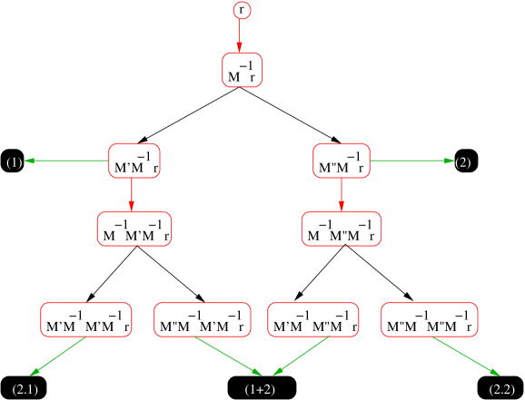
Figure 2: Representing the evaluation tree for NLS. The root node is a random vector $r$, internal nodes stand for vectors formed by application of a matrix on a vector, and leaves (in black) stand for scalars. Here every vertical edge represents the application of $M^{-1}$ on a vector (which is the costliest part of the computation), every horizontal edge stands for dotting with $r^{\dagger}$ to give a scalar, and other edges for application of $M^{\prime}$ (left slanting) or $M^{\prime\prime}$ (right slanting). The Steiner problem corresponds to finding the minimum cost of evaluating a given set of scalars. In the compact representation at the right, the horizontal edges have been contracted to bring the leaf nodes into the body of the tree and vertical edges have been contracted to a point. Note that the redundancy in the computation of $\lfloor 1\oplus 2\rceil$ (also written as 21) can be used as a check of the program.

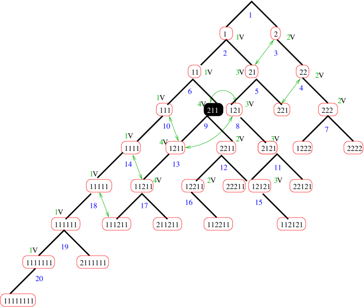
Figure 3: The evaluation tree for 8th order NLS requires 20 matrix inversions (numbered at the branches in the tree) and one extra node (in black). Since leaves are denser on the right of the tree, evaluating the inverses from right to left results in the use of less memory in the form of vectors to be stored. An assignment of vectors is shown (1V, 2V etc.), which uses only 4 intermediate storage vectors. Bidirectional arrows connect quantities that serve as checks of the program.

The traces are evaluated through a noisy technique—

$${\rm Tr}\,A=\overline{r^{\dagger}Ar}/\overline{r^{\dagger}r},$$ (11)

where the bar denotes averaging over random vectors $r$. An unbiased measurement is provided for ensembles of random vectors which satisfy the conditions—

$$\overline{(r^{\alpha}_{i})^{*}r^{\beta}_{j}}=N\delta_{\alpha\beta}\delta_{ij}$$ (12)

where $\alpha$, $\beta$ label the vector, $i$, $j$ label the components, and $N$ may depend on the ensemble but is independent of either index. The matrix $A$ consists of a product of $M^{-1}$, $M^{\prime}$ and $M^{\prime\prime}$ such that there is one $M^{-1}$ for each of the other two. The costliest part of the evaluation is the computation of $M^{-1}$ acting on a vector. While evaluating a certain (fixed) set of traces, we need to minimise the number of matrix inversions.

We represent this problem through a directed graph without cycles. Each internal node of the graph contains a vector, and each leaf contains a scalar. The root node is the random vector $r$, and every other internal node is obtained by the action of some matrix on $r$. Since each vector is obtained from another by the action of either $M^{\prime}M^{-1}$ or $M^{\prime\prime}M^{-1}$, the internal nodes form a binary tree. To count the cost of any operation we separate the action into a single $M^{-1}$ followed by either $M^{\prime}$ or $M^{\prime\prime}$. Each internal node (except the root) gives rise to a leaf by dotting it with $r^{\dagger}$. Since this action is the stochastic evaluation of a trace, several internal nodes (differing by cyclic permutations of the operations) may connect to each leaf. A representation of the evaluation tree up to level 2 is given in Figure 2. A compressed representation, also shown in Figure 2, is obtained by collapsing together the nodes containing a vector $v$ and the vector $M^{-1}v$, by writing $1$ for each $M^{\prime}$, $2$ for each $M^{\prime\prime}$ and never writing $M^{-1}$.

Our problem is— given a set of target leaf nodes, find the path on the tree using the minimum number of $M^{-1}$ which evaluates these leaves. This is one version of a problem known in the computer science literature as the group Steiner problem on directed graphs, for which a solution has been given recently steiner . The computer science interest arises from the fact that the general problem is known to be in the class of NP complete problems.

Since our problem size is small, we do not use the general algorithm, but a heuristic which shares the idea of “bunching” with that algorithm, uses the structure specific to this problem, and is easily implemented in wetware. Given the set of matrix elements, write down all strings which have to be generated, and group each with all its cyclic permutations. For each set of strings of length $\ell$, starting from the largest, enumerate the suffixes of length $\ell-1$. Choose that representation in which the suffixes are common at the nearest possible level. This is the central heuristic— bunch the strings by largest suffixes. Build this back all the way to the empty string, backtracking only if there is insufficient bunching close to the root. This gives an evaluation tree. Run over all such trees and find the ones with lowest cost.

For the 4th order problem this yields:

$$(1) : 1,$$

$$(2) : 2,$$

$$(2\cdot 1) : 1\underline{1},$$

$$(1\,{\oplus}\,2) : 12,\;2\underline{1},$$

$$(2\cdot 2) : 2\underline{2},$$

$$(3\cdot 1) : 1\underline{11},$$

$$(2\cdot 1\,{\oplus}\,2) : 112,\;121,\;2\underline{11}$$

$$(4\cdot 1) : 1\underline{111},$$

The underlined suffixes are used in the evaluation. The tree is identified from bottom up, but evaluated top down. A solution for the 8th order problem is given in Figure 3.

There seems to be a large degree of redundancy in the most efficient evaluation. This can be used to minimize the number of internal nodes not connected to the target leaf set. Even after this is done, there seems to be further degeneracy, and this can be utilised to minimize the breadth of the tree, since that determines the number of vectors needed in the evaluation.

Sometimes only one of the two branches is needed in the evaluation. Since both branches can be generated at nearly the same cost as one, the other branch can then be used to check the numerical accuracy of the procedure. Such possible checks are marked by bi-directional arrows in Figure 3.

III.2 Inverting the fermion matrix

Figure 4: The evolution of the norm of the residual, $|r_{n}|^{2}$ against the number of conjugate gradient iterations, $n$. This figure shows the computation on a typical gauge configuration at $T=1.05T_{c}$ using one random vector for the full evaluation tree of the 8th order NLS. In Method 1 $n$ increases as one proceeds down the tree. In Method 2 $n$ remains almost constant (see the thick line).

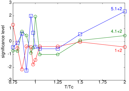
Figure 5: Results of inversion with $\epsilon=10^{-6}$ with method 1 (full lines) and with $\epsilon=10^{-3}$ with method 2 (dotted lines). The latter are significantly different for $\langle\overline{\psi}\psi\rangle$ and $\chi_{\pi}$, but not for the traces ${\cal O}_{n}$. Inversions with $\epsilon=10^{-4}$ with method 2 are indistinguishable from the full lines on the scale of this figure. The panel on the right displays the accuracy of the inversions as one proceeds down the evaluation tree. The significance level is defined as the difference of two evaluations of the same trace divided by the error in the difference.

The fermion matrix inversion is done through a conjugate gradient method. The most time consuming part of this problem is the matrix multiplication $M^{\dagger}Mx$. A huge gain could be obtained if the multiplication could be speeded up in any way. Each matrix multiplication involves $V$ diagonal terms and $2dV$ off-diagonal terms (where $V$ is the number of sites, and $d$ the number of dimensions). Each diagonal term involves $N_{c}$ multiplications. Each off-diagonal term involves $2N_{c}^{2}$ operations ($N_{c}^{2}$ multiplications and $N_{c}^{2}$ additions). Hence the total operation count for the double matrix multiplication is $VN_{c}(1+4dN_{c})$.

One consequence of this is that ‘improved’ methods such as preconditioning or deflation are not of much use unless the number of matrix multiplications can be cut down drastically. For example, in our application where the same matrix is applied repeatedly on many different vectors, one might expect deflation to work wonders saad . However, this requires two double matrix multiplications per step and hence actually performs worse.

The simplest solution, and the one that seems to work best, is to tune the stopping criterion. In Figure 4 we show the performance of two different criteria—

1. Method 1 is to require the norm of the residual, $|r_{n}|^{2}<\epsilon V$. Since each inversion increases the norm of the right-hand side, through the 20 inversions required for evaluating all the traces, the CG has to take increasingly larger number of steps, $n$, for convergence.

2. Method 2 is to require the norm of the residual, $|r_{n}|^{2}<\epsilon|r_{0}|^{2}$. As shown in the figure, this seems to keep $n$ almost fixed as one proceeds through the evaluation tree.

There is really no a priori reason for the two stopping criteria to give equally accurate results with the same value of $\epsilon$. However, we see that for $\epsilon\leq 10^{-4}$ the results do not differ for the ${\cal O}_{n}$’s (they do for $\langle\overline{\psi}\psi\rangle$), while method 2 takes less CPU time. To have some understanding of this, we note that since any matrix is diagonalised by a bi-unitary transformation, we can write $M=U^{\dagger}DV$, where $D$ is diagonal, and $U$ and $V$ are unitary matrices. Similarly, $M^{\prime\prime}=W^{\dagger}D^{\prime\prime}X$, giving

$${\rm Tr}\,M^{-1}M^{\prime\prime}={\rm Tr}\,D^{-1}UW^{\dagger}D^{\prime\prime}XV^{\dagger}=\sum_{ij}\frac{d_{jj}^{\prime\prime}}{d_{ii}}(UW^{\dagger})_{ij}(XV^{\dagger})_{ji}$$ (14)

The triangle inequality can then be used to bound

$$|{\rm Tr}\,M^{-1}M^{\prime\prime}|\leq\sum_{ij}\left|\frac{d_{jj}^{\prime\prime}}{d{ii}}(UW^{\dagger})_{ij}(XV^{\dagger})_{ji}\right|\leq\left\{\sum_{i}|1/d_{ii}|\right\}\,\left\{\sum_{i}|d_{ii}^{\prime\prime}|\right\}.$$ (15)

Since every element of an unitary matrix is bounded by unity, we get the second bound above by inserting unity for these matrix elements. However, this bound is too rough. If it is (nearly) saturated then the trace would depend on the stopping criterion as strongly as $\langle\overline{\psi}\psi\rangle={\rm Tr}\,M^{-1}$, contrary to observation. Therefore it seems likely that the structure of the unitary matrices plays a role in reducing the bound. In particular, we note that the low eigenvalues of $M$, $d_{ii}\leq\rho$ can be killed only by eigenvalues of $M^{\prime\prime}$. This can happen if the unitary matrices $WU^{\dagger}$ and $XV^{\dagger}$ are nearly block-diagonal in this subspace (they are exactly block-diagonal in the vacuum or in the presence of stationary gauge fields, when the Dirac operator becomes separable). In other words, the observed lack of sensitivity to small eigenvalues of $M$ can be understood if every near-zero mode of $M$ is also a near-zero mode of $M^{\prime\prime}$.

IV Lattice simulations and results

IV.1 Parameters and simulations

$\beta$	$\;m$	$T/T_{c}$	$4\times 8^{3}$		$4\times 10^{3}$		$4\times 12^{3}$		$4\times 16^{3}$		$4\times 24^{3}$
			$N_{\rm stat}$	$\tau_{\rm max}$	$N_{\rm stat}$	$\tau_{\rm max}$	$N_{\rm stat}$	$\tau_{\rm max}$	$N_{\rm stat}$	$\tau_{\rm max}$	$N_{\rm stat}$	$\tau_{\rm max}$
$5.20$	$\;0.033$	$0.75\pm 0.02$	86	25	28	20	172	14	89	15	—	—
$5.22$	$\;0.03125$	$0.8\pm 0.02$	206	19	193	14	94	14	84	15	—	—
$5.24$	$\;0.0298$	$0.85\pm 0.01$	89	14	43	14	271	15	210	15	—	—
$5.26$	$\;0.02778$	$0.9\pm 0.01$	144	29	70	59	50	21	65	17	63	12
$5.275$	$\;0.02631$	$0.951\pm 0.01$	115	34	110	112	98	42	26	35	56	17
$5.2875$	$\;0.025$	$1.00\pm 0.01$	44	207	22	362	56	217	51	131	123	43
$5.30$	$\;0.0238$	$1.048\pm 0.01$	4	279	178	114	110	41	111	42	—	—
$5.35$	$\;0.02$	$1.25\pm 0.02$	139	6	—	—	—	—	73	9	—	—
$5.425$	$\;0.01667$	$1.65\pm 0.06$	1146	6	—	—	—	—	112	7	—	—
$5.54$	$\;0.0125$	$2.15\pm 0.10$	1648	6	—	—	49	6	313	4	—	—

Table 1: The couplings $\beta$ and bare quark masses $m$ at which the simulations were performed. The temperature scale, $T/T_{c}$, is given in the $\overline{\rm MS}$ scheme, with error assignment as discussed in the text. The bare quark mass at all temperatures correspond to $m=0.1T_{c}$. The statistics collected in each simulation, $N_{\rm stat}$, is given in terms of the longest autocorrelation time, $\tau_{\rm max}$, measured in that simulation in MD time units. The trajectory lengths are 1 MD time unit on the $4\times 8^{3}$ lattice and scaled up in proportion to the length of the spatial lattice, i.e., growing to 3 MD time units on the $4\times 24^{3}$ lattice.

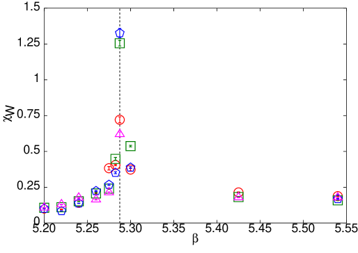
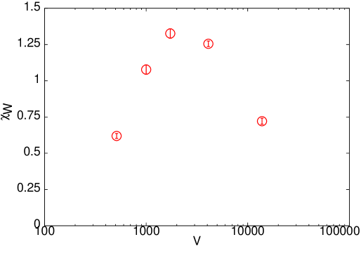
Figure 6: The Wilson line susceptibility, $\chi_{L}$, shown on the left as a function of the bare coupling, $\beta$ on lattice sizes of $8^{3}$ (triangles), $12^{3}$ (pentagons), $16^{3}$ (boxes) and $24^{3}$ (circles). It is clear that $\beta=5.2875$ does not locate the exact position of the peak on the larger volumes. This is also indicated in the figure on the right, which depicts $\chi_{L}$ at a fixed $\beta=5.2875$ as a function of $V$.

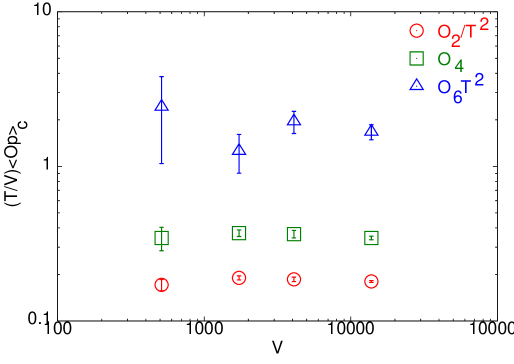
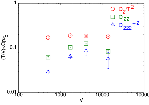
Figure 7: The panel on the left shows operator expectation values $\langle{\cal O}_{n}\rangle$ as functions of the volume at $T=0.75T_{c}$. The panel on the right shows that the connected parts $\langle O_{22}\rangle_{c}$, and $\langle O_{222}\rangle_{c}$ at $0.75T_{c}$ scale with the correct power of $V$.

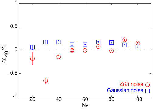
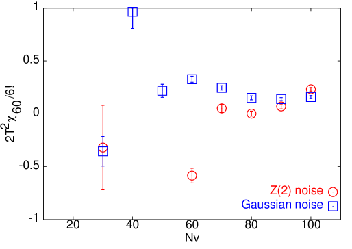
Figure 8: A comparison of Gaussian noise (boxes) and $Z_{2}$ noise (circles) for the evaluation of the NLS $\chi_{40}$ (left panel) and $\chi_{60}$ (right panel) at $0.75T_{c}$ on a $4\times 16^{3}$ lattice. Gaussian noise requires less vectors for stable evaluation of these quantities.

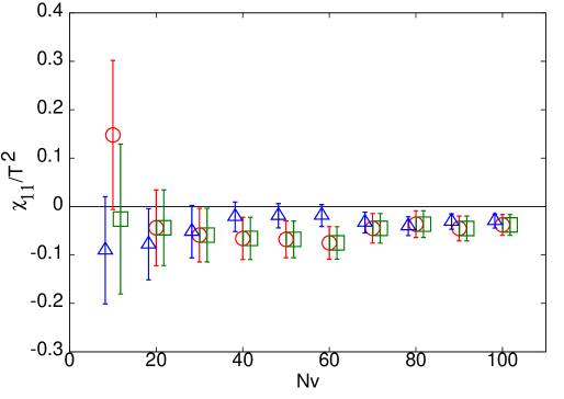
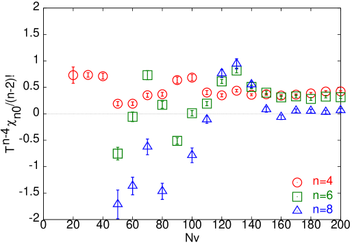
Figure 9: Estimates of $\chi_{11}/T^{2}$ as functions of the number of vectors $N_{v}$ for $0.75T_{c}$ on a $4\times 24^{3}$ lattice. Shown are the estimates using Gaussian noise and CG stopping criterion of $10^{-4}$ (circles) and $10^{-6}$ (boxes) in Method I and $Z_{2}$ noise with CG stopping criterion of $10^{-4}$ in Method I (triangles). $N_{v}$ are chosen to be multiples of 10, but some of the points are displaced slightly in the x-direction for improved visibility. The panel on the right shows $\chi_{n0}$ as a function of $N_{v}$ for $n=4$ (circles), 6 (boxes) and 8 (triangles). This data was collected at $0.75T_{c}$ on a $4\times 10^{3}$ lattice with Gaussian noise and $\epsilon_{CG}=10^{-4}$.

All the simulations reported in this paper were carried out at the lattice spacing $a=1/4T$, corresponding to lattices with temporal extent $N_{t}=4$. We used the R-algorithm in the simulations and chose the conjugate gradient stopping criterion to be Method 1 of Section III with $\epsilon=10^{-5}$. The finite temperature crossover at this cutoff has been determined to be at the coupling $\beta=5.2875\pm 0.0025$ gotttc , which therefore corresponds to the cross over temperature $T_{c}$ at zero $\mu$. We have improved the bound on the cross-over coupling, as we report later in this section.

We have set the scale by using plaquette values to define a renormalized coupling scale in a series of exploratory computations on small lattices ($16^{4}$) at $T=0$, using trajectory lengths of one molecular dynamics (MD) unit. The typical statistics utilised for scale setting was about 500 such trajectories, of which the initial 200 were discarded for thermalization. During the scale setting the input bare quark mass was varied until a self-consistent determination of the scale showed that $m/T_{c}=0.1$ within statistical errors. A two-loop analysis of the scale shows several sources of uncertainty. Statistical uncertainties can be easily made small, and with our statistics they are of the order of 3–6 parts per thousand. Harder to control are the differences between various renormalization schemes and the scatter due to errors in the estimate of the critical coupling. The latter induces an error of slightly over 1% in the scales. Differences between different renormalization schemes indicate that $a=1/4T_{c}$ is too coarse for 2-loop formulæ to work with high precision. This problem is also known in the quenched theory, where it was seen that a higher order correction was needed to achieve scaling scale . Here we quantify this uncertainty by taking the scatter between the scale determination through the E, V and $\overline{\rm MS}$ schemes. The uncertainty defined in this manner is within 2% of the value in the $\overline{\rm MS}$ scheme for $T$ within 25% of $T_{c}$, but grows rapidly beyond, upto about 10% at the value of $\beta_{c}$ determined at $N_{t}=8$ for $m/T_{c}=0.1$. Since the critical end point lies close to $T_{c}$, we decided not to do an extensive set of $T=0$ simulations to control the scale further by extracting higher order terms in the $\beta$-function. The combined statistical and systematic errors in the determination of $T/T_{c}$ are shown in Table 1.

Hadron masses have been determined earlier at the critical coupling gottm . It was found that $m_{\pi}/m_{\rho}=0.31\pm 0.01$, which is somewhat larger than in nature. $T_{c}$ could be given in physical units by noting that $m_{\rho}/T_{c}=5.4\pm 0.2$. Further evidence that lattice spacings are still fairly coarse can be seen by noting that the nucleon is too heavy, since $m_{N}/m_{\rho}=1.8\pm 0.02$. Pushing towards the continuum will be a necessary future step.

The simulation parameters and statistics are shown in Table 1. The MD trajectory was chopped into time steps of length 0.01, and the full trajectory was chosen to be 1 time unit for the $4\times 8^{3}$ runs. As the spatial size, $N_{s}$ of the lattice changed, the trajectory length was changed in proportion to $N_{s}$. An earlier study had shown such a tuning of the trajectory length to be useful in controlling the growth of autocorrelations mdtau . We found that the number of iterations in the conjugate gradient algorithm remained unchanged as the spatial volume increased at fixed $T$.

The pseudo-critical point is usually identified by the Wilson line susceptibility, $\chi_{L}$, the chiral susceptibility, $\chi_{m}$, which is the second derivative of the free energy with respect to the quark mass karsch , or autocorrelations of various measurements. All of these are expected to peak at $T_{c}$. If the point is critical, then one expects these quantities to grow as a power of the volume, $V$. If, on the other hand, there is a cross over, then these peak heights should saturate at large enough $V$. Also, different quantities could peak at somewhat different temperatures even for $V\to\infty$ ray .

In Figure 6 we show a measurement of $\chi_{L}$ at the couplings we have used. The drop in the peak of $\chi_{L}$ on the largest $V$ is clear indication that $\beta=5.2875$ is not the location of the peak in the thermodynamic limit. In order to bracket the position of the peak we have run separate simulations on $4\times 12^{3}$ and $4\times 16^{3}$ lattices at nearby couplings with bare quark mass fixed at $ma=0.025$. Collecting statistics from about 30 to 50 independent configurations at each coupling, we find that the finite volume shift in the peak is less than $\Delta\beta=0.00125$ for $N_{s}=16$. This corresponds to an error of 1% or less on $T_{c}$.

Such a shift is not of significant concern for our study since the dominant systematic error in the scale setting comes from the fact that the lattice spacings for $N_{t}=4$ in the temperature range of interest are too coarse for 2-loop scaling to work— improving the estimate of $T_{c}$ beyond the present 1% level of scale does not improve the total systematic error by 1%. Of course, as a consequence, these data cannot yet be used to check whether there is a phase transition or a cross over in the $\mu=0$ theory. This is an interesting but separate problem edwin ; digiacomo . It might be useful in future to explore a narrow region of $\beta$ near the peak in greater detail to track the growth of $\chi_{L}$ with $V$ and give a definitive answer to this question.

Several local gauge operators as well as quark operators such as the chiral condensate were measured once per trajectory. The longest autocorrelation, $\tau_{\rm max}$, in these measurements was used to set the scale of autocorrelations. It was seen that $\tau_{\rm max}$, when measured in MD time units, was roughly independent of $N_{s}$ at fixed $T$, as expected from the scaling of the trajectory length mdtau . As a consequence of these scalings, the time taken for generating one new configuration scaled approximately as $N_{s}^{5}$ at fixed $T$ in thermal equilibrium.

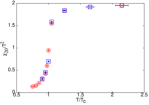
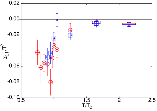
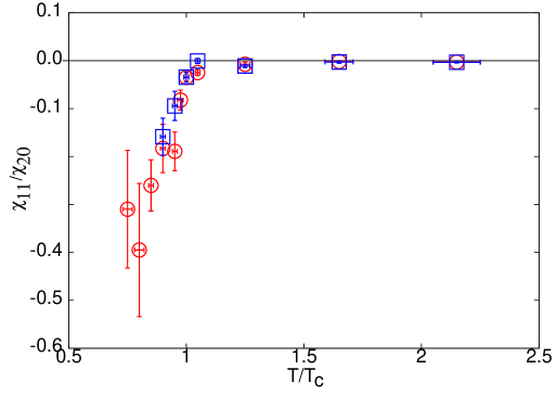
Figure 10: The quark number susceptibilities on lattice sizes $4\times 16^{3}$ (circles) and $4\times 24^{3}$ (boxes). The first panel shows $\chi_{2}/T^{2}$, the second $\chi_{11}/T^{2}$, and the third the ratio.

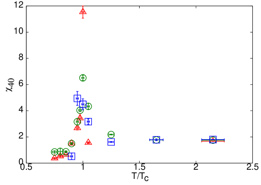
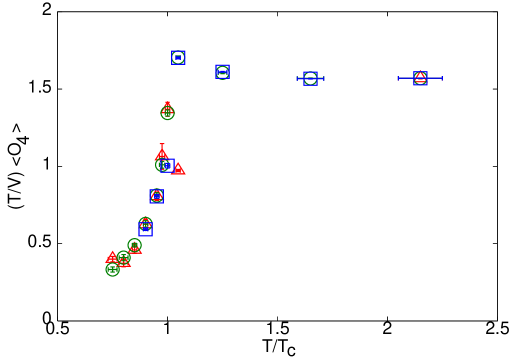
Figure 11: A fourth order QNS and some connected parts on lattice sizes $4\times 12^{3}$ (triangles), $4\times 16^{3}$ (circles) and $4\times 24^{3}$ (boxes). The first panel shows $\chi_{40}$ and the second $(T/V)\langle{\cal O}_{4}\rangle$.

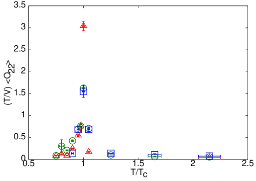
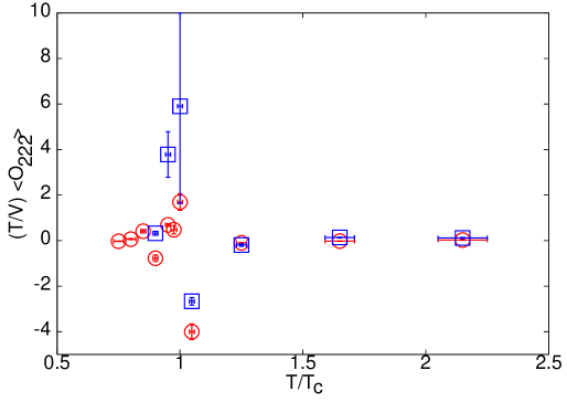
Figure 12: Some connected parts on lattice sizes $4\times 16^{3}$ (circles) and $4\times 24^{3}$ (boxes). The first panel shows $(T/V)\langle{\cal O}_{22}\rangle$. The second panel shows a model cross-over (full line) with first (dashed) and second (dotted) derivatives. The third panel shows $(T/V)\langle{\cal O}_{222}\rangle_{c}$. Note the similarities between data and model.

IV.2 Noise and measurement

Full control over errors in determining the non-linear susceptibilities is crucial for the job of extrapolation to non-zero $\mu$. The major source of numerical errors is the numerical cancellation of divergences which go as powers of the volume in order to get a finite result. One part of this program is the identification of primitive volume independent quantities— the connected parts of fermion-loop disconnected operators, some of which were enumerated in Section II.1. In this section we complete the program by showing that some choice of the noise ensemble works better than others liu , and that the number of vectors is the crucial parameters, not the choice of the conjugate gradient stopping criterion.

In Figure 7 we show the easiest part of this program— the scaling with volume of the expectation values $(T/V)\langle O_{n}\rangle$. These are fairly easy to handle because the operators have no disconnected pieces and there are no divergences to cancel. We find that the values and the error estimates are very stable against the choice of the conjugate gradient stopping criterion, in method I we can change $\epsilon$ from $10^{-4}$ to $10^{-6}$ without making a change to these quantities. There may be a little volume dependence in going from $N_{s}=8$ to $N_{s}=12$ lattices, but this saturates for $N_{s}$ between 12 and 24. The errors become larger as $n$ increases.

We found that, in agreement with expectations, the disconnected pieces of traces such as $\langle{\cal O}_{ij\cdots}\rangle$ grow with volume as a power equal to the number of fermion-line disconnected pieces in the operator. However, as shown in Figure 7, the connected part grows roughly linearly with volume. The residual volume dependence is small, and the fact that $(T/V)\langle{\cal O}_{222}\rangle_{c}$ decreases with $V$ shows that the cancellation of the leading divergent pieces has been performed satisfactorily. These results have been obtained with 100 noise vectors drawn from a Gaussian ensemble.

We have made further tests of the effect of the choice of the noise ensemble, as shown in Figure 8. It seems that it is preferable to use Gaussian noise rather than $Z_{2}$ noise, since the former is more stable against changes in the number of random vectors used. Since quite the opposite conclusions have been presented in the literature, albeit for different measurements liu , we investigated this a little further. It seems that indeed $Z_{2}$ noise performs better for single traces, as in the measurements of $\langle{\cal O}_{n}\rangle$. However, the measurement of products of traces such as $\langle{\cal O}_{ij\cdots}\rangle$ is cleaner with Gaussian noise.

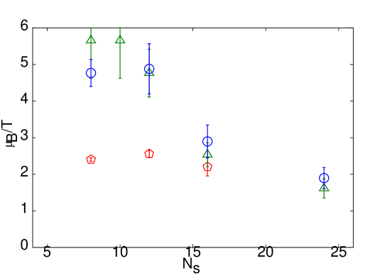
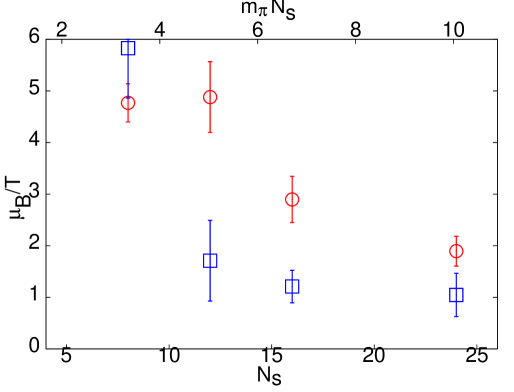
Figure 13: The radius of convergence of the series expansion for $\chi_{20}$. The first panel shows $r_{6}$ at $T/T_{c}=0.9$ (pentagons), 0.95 (circles) and 1 (triangles). The second panel shows results at $T/T_{c}=0.95$ for $r_{4}$ (circles) and $r_{6}$ (boxes).

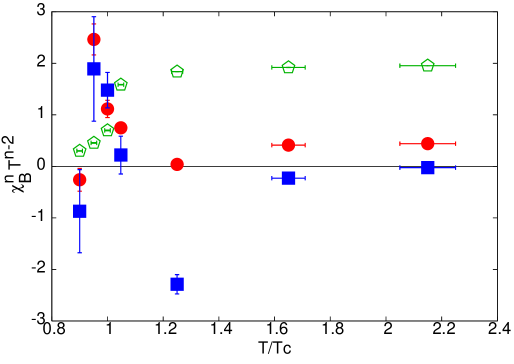
Figure 14: We show the dimensionless series coefficients, $\chi_{B}^{n}T^{n-2}$ (eq. 4), obtained on $4\times 24^{3}$ lattices, for $n=0$ (pentagons), $n=2$ (circles) and $n=4$ (boxes). The $n=2$ coefficients have been divided by 2 and the $n=4$, by 12, in order to bring them all to roughly the same scale.

Figure 15: $\chi_{20}(\mu_{B})/T^{2}$ obtained using merely two terms in the Taylor expansion already shows the qualitative change above $T=0.9T_{c}$. The 66% confidence intervals for the extrapolation are shown for $T_{c}$ (full lines), $0.95T_{c}$ (dash-dotted) and $0.9T_{c}$ (dashed) from computations on a $4\times 24^{3}$ lattice.

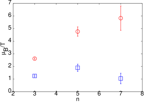
Figure 16: We show the radii of convergence as a function of the order of the expansion at $T=0.95T_{c}$ on a $4\times 8^{3}$ lattice (circles) and a $4\times 24^{3}$ lattice (boxes). The panel on the left shows $\rho_{n}$ and the one on the right is for $r_{n}$.

The two final issues to be resolved are the role of the accuracy in the conjugate gradient, and the number of vectors required for measurements. In Figure 9 we show that the choice of the CG stopping criterion, $\epsilon_{CG}$, does not significantly affect the choice of $N_{v}$. It is also clear from this figure that larger values of $N_{v}$ are required for the higher order measurements. In particular, $N_{v}=100$ seems to suffice for measurements up to the 4-th order, whereas $N_{v}=200$ is required beyond that for measurements up to the 8-th order, in the hadronic phase. In fact, $N_{v}$ also depends on the lattice size. On smaller lattices $N_{v}=200$ seem to suffices, but this grows with lattice size and on the $4\times 24^{3}$ lattices one needs $N_{v}=500$ below $T_{c}$. Above $T_{c}$, $N_{v}=100$ seems to suffice for all the measurements and lattice sizes.

IV.3 Susceptibilities and radii of convergence

In this subsection we present results on the temperature dependence of the linear and non-linear quark number susceptibilities. Comparable data on the linear QNS in the high temperature phase were presented in pushan . In figure 10 we present data for $\chi_{20}/T^{2}$ and $\chi_{11}/T^{2}$. Some volume dependence is visible in the immediate vicinity of $T_{c}$. The high temperature behaviour is compatible with the predictions of bir ; alexi . The results are also completely compatible with earlier results in pushan after correcting for a division by an extra factor of $(T/V)$ for $\chi_{11}/T^{2}$ reported there. Comparison with the recent results of milc are harder to perform since the actions are different. As a result, such a comparison can be meaningfully performed only after taking the continuum limit.

There is a clear qualitative difference in $\chi_{11}$ above and below $T_{c}$. Above $T_{c}$ it is significantly easier to measure, is small and compatible with zero. Below, and in the vicinity of $T_{c}$, it is possibly larger, but much harder to measure because of fluctuations. The ratio $\chi_{11}/\chi_{2}$, taken at $\mu_{B}=0$, quantifies the magnitude of the fermion sign problem at small $\mu_{B}$, as discussed in Section II. This ratio is also shown in Figure 10. It is clear that the fermion sign problem is negligible at higher temperatures. The success of modern extrapolation methods at finite $\mu$ fk ; pressure ; biswa is, at least partially, due to this. Due to the rapid increase in phase fluctuations on lowering $T$, visible in Figure 10, any extrapolation technique would be hard to use significantly below the lowest temperatures we have used. Since $\chi_{11}$ depends strongly on the pion mass, we expect phase fluctuations to pose greater difficulties as one approaches the physical pion mass. Conversely, the sign problem would be easier to deal with in simulations at higher pion masses, such as biswa .

We show the fourth order NLS, $\chi_{40}$, in Figure 11 for our three largest lattice volumes. Away from the critical region the volume dependence is seen to be negligible. In the critical region, however, $\chi_{40}$ exhibits behaviour similar to that of $\chi_{L}$ (Figure 6). The susceptibility peaks near $T_{c}$ and shows pseudo-critical behaviour, since the near-critical region visibly shrinks with increasing volume. Since $\chi_{40}$ decreases with $V$ at fixed $\beta=5.2875$, we again have evidence that the cross-over coupling is near this, but not exactly here.

Further insight into the nature of this peak comes from examining the other NLS at this order. It turns out that $\chi_{22}$ also has a similar sharp peak, whereas $\chi_{31}$ is much smoother. These lead us to examine the connected parts which contribute at this order (see eq. 9). We found that $(T/V)\langle{\cal O}_{4}\rangle$, shown in Figure 11, seems to behave almost as a (pseudo) order parameter for the crossover at $T_{c}$. In this it behaves like $\chi_{20}/T^{2}$ and, indeed, like all the single traces $(T/V)\langle{\cal O}_{n}\rangle$ that we have examined. The peaking behaviour is essentially due to a similar peak in $(T/V)\langle{\cal O}_{22}\rangle_{c}$, which we have displayed in Figure 12.

Note that ${\cal O}_{2}$ is a composite bosonic operator. It may be possible to write down effective long-distance theories in which it is treated as a field operator whose expectation value shows the correct cross over behaviour. In that case $\langle{\cal O}_{22}\rangle_{c}$ would be the susceptibility of this field, and being proportional to the temperature derivative of $\langle{\cal O}_{2}\rangle$, would peak, as observed. In fact, one can push this idea further, and examine the expectation values $\langle{\cal O}_{222}\rangle_{c}$. In such an effective theory one would find this to be proportional to the next derivative of $\langle{\cal O}_{2}\rangle$. Then the $T$-dependence of these quantities at $\mu_{f}=0$ would have the shapes shown in the second panel of Figure 12. In fact, the data, shown in the final panel of Figure 12, does show the same qualitative behaviour. Thus, the cross-over at $T_{c}$ can be probed by any of these connected parts.

There is significant volume dependence in the close vicinity of $T_{c}$, although for $T\leq 0.95T_{c}$ one is clearly outside the pseudo-critical region, and the volume dependence is weak. Within the pseudo-critical region the peak of $\langle{\cal O}_{22}\rangle_{c}$ is seen to have the same qualitative behaviour as the peak of $\chi_{L}$ shown in Figure 6, including similar evidence for finite volume shift in the cross over coupling. There are consequent effects on the higher order connected parts, as shown in Figure 12.

With the NLS at hand, we construct the Taylor expansion of the diagonal QNS, $\chi_{20}(\mu_{B})$, where the coefficients are given in eq. (4). Radii of convergence can be obtained for the series expansion $f(x)=\sum f_{2n}x^{2n}$ using two definitions—

$$\rho_{n}=\left|\frac{f_{0}}{f_{2n}}\right|^{1/2n},\qquad{\rm and}\qquad r_{n}=\left|\frac{f_{2n}}{f_{2n+2}}\right|^{1/2},$$ (16)

At large $n$ both definitions should be equivalent, although for many series it is known that the latter gives somewhat smoother approach to the limit of $n\to\infty$. Also, at a critical point, one may extrapolate the latter to the limit $n\to\infty$ by a fit to a $1/n$ behaviour gaunt . We apply these definitions to the series for the baryon number susceptibility (see above eq. 4).

In Figure 13 we display the radii, $r_{4}$ and $r_{6}$, at several different temperatures as a function of $N_{s}$: the volume dependence is strong. For $0.95\leq T/T_{c}\leq 1$, the radii roughly agree with the estimate of the critical end point in fk for $N_{s}$ comparable to those used in that study. However, as the volume increases, the radius of convergence drops. The magnitude of the finite volume effects is parametrized by the pion Compton wavelength, and for $m_{\pi}N_{s}\geq 5$–6 one finds that these effects saturate. This is in accord with the discussion in Section II.2. Similar saturation of finite size effects has been seen in other measurements in the chiral sector at similar values of $m_{\pi}N_{s}$ ray .

At temperatures below $0.95T_{c}$ the radius of convergence falls quite dramatically. However, examination of the series coefficients shows that in this lower range of temperatures the 6th order coefficient, $\chi_{B}^{6}$, is negative (see, Figure 14). Thus the radius of convergence does not indicate a divergence. Rather, it shows that at this temperature $\chi_{20}(\mu_{B})<0$, thus violating thermodynamic stability, and therefore indicating that higher order terms in the expansion become necessary. This is consistent with the increase in the ratio $\chi_{11}/\chi_{20}$ at these $T$ (see Figure 10). At temperatures between $T_{c}$ and $0.95T_{c}$, the character of the expansion is quite different, with all the Taylor coefficients being positive. As discussed earlier, when this is true the series diverges on the real $\mu_{B}$ axis. The qualitative difference in these two expansions is already visible at low order, and is illustrated in Figure 15. Note that a figure like this illustrates whether or not there is a divergence, but since it shows the sum of a finite number of terms, it cannot show anything special happenning at the radius of convergence.

In Figure 16 we show the variation of the two different definitions of the radius of convergence, $\rho_{n}$ and $r_{n}$, with the order $n$. On our smallest lattice, $4\times 8^{3}$, the successive estimates diverge, and the two sets of estimates are compatible at the 2-$\sigma$ level. After the cross over to large volume behaviour, the estimates stabilize with order, being nearly independent of $n$. Also $\rho_{n}$ and $r_{n}$ are in close agreement with each other. The radius of convergence extrapolated to all orders at $T^{E}=0.95T_{c}$ gives $\mu^{E}/T^{E}=1.1\pm 0.2$.

If we assume that the end point is in the Ising universality class, then the finite volume shift in the end point is given by

$$\mu^{E}(V)=\mu^{E}(\infty)+\frac{a}{V^{1/\delta}},\qquad{i.e.}\qquad\mu^{E}(V)-\mu^{E}(V^{\prime})=\frac{a}{V^{1/\delta}}-\frac{a}{{V^{\prime}}^{1/\delta}},$$ (17)

where $\delta=5$ is the 3-d Ising magnetic exponent and $V=N_{s}^{3}$. Using the data exhibited in Figure 13 for $N_{s}=16$ and 24, which are both above the crossover, it is easy to check that the finite volume shift in $\mu^{E}$ is bounded by the statistical error in the estimate for $N_{s}=24$. In view of this, we quote the estimate and its error obtained for the $N_{s}=24$ lattice as the estimate in the thermodynamic limit.

V Summary and discussion

The main result we present in this paper is the strong volume dependence of location of the critical region, leading to a substantially smaller estimate of $\mu_{B}^{E}$ on large volumes than before. We began by constructing the Taylor expansion for the quark number susceptibility, $\chi_{20}(T,\mu_{B})$, for $N_{f}=2$ QCD at for several large volumes. The leading ($\mu_{B}$ independent) term of the series is the quark number susceptibility (QNS) which has received extensive attention recently pushan ; valence ; milc ; bir ; alexi ; mustafa . The remaining Taylor coefficients involve the non-linear susceptibilities (NLS) which were defined in pressure . We have taken the series up to the 6th order term, which involves 8th order NLS. A systematic and efficient procedure for generating and computing the quark number susceptibilities at any order was presented in Sections II and III.

$m_{\rho}/T_{c}$	$m_{\pi}/m_{\rho}$	$m_{N}/m_{\rho}$	$N_{s}m_{\pi}$	flavours	$T^{E}/T_{c}$	$\mu_{B}^{E}/T^{E}$	reference
5.372 (5)	0.185 (2)	—	1.9–3.0	2+1	0.99 (2)	2.2 (2)	fktwo
5.12 (8)	0.307 (6)	—	3.1–3.9	2+1	0.93 (3)	4.5 (2)	fk
5.4 (2)	0.31 (1)	1.8 (2)	3.3–10.0	2	0.95 (2)	1.1 (2)	this work
5.4 (2)	0.31 (1)	1.8 (2)	3.3	2	—	—	owe
5.5 (1)	0.70 (1)	—	15.4	2	—	—	biswa

Table 2: Summary of critical end point estimates— the lattice spacing is $a=1/4T$. $N_{s}$ is the spatial size of the lattice and $N_{s}m_{\pi}$ is the size in units of the pion Compton wavelength, evaluated for $T=\mu=0$. The ratio $m_{\pi}/m_{K}$ sets the scale of the strange quark mass. As the mass scales indicate, the lattice spacings and $u$ and $d$ quark masses of fk and this work are comparable. The numbers in brackets indicate the errors on the least significant digit. Since no estimates of the critical end point are quoted in biswa ; owe , the comparison is more complicated, and is described in the text.

The main thrust of this work is to approach the large volume limit. From the point of view of thermodynamics, this limit has to be taken in order to decide whether rapid changes in certain quantities and peaks in others are due to critical behaviour, cross over or a first order phase transition. For the $\mu_{B}=0$ cross over at $T_{c}$, good progress has been made edwin . However, due to questions such as the magnitude of the shift in the critical coupling, and the absence of evidence for peaking of different susceptibilities at slightly different points, an unqualified answer is still not available. Note, however, the remarkably high accuracy in the measurement of $T_{c}$ that is possible even without answering this question. The situation is similar at critical points. It is usually much easier to identify the critical point (assuming it is critical) than it is to “prove” criticality through extensive analysis. In this work we have shown that there is a minimum lattice size that one should use in order to get a reliable estimate of the position of the critical end point. Further work involved in “proving” criticality by studying detailed finite size effects, with substantially larger lattice volumes and extracting critical indices, is beyond our present computational capability and is left for the future.

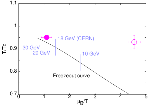
Figure 17: The phase diagram and the freeze-out curve superimposed. The filled circle denotes the estimate of the critical point which was obtained in this work. The open circle is an earlier estimate from fk using smaller lattices and nearly the same quark mass as in this work (see the text for a discussion of their comparability). The freezeout curve pvt has been converted for this figure using a value of $T_{c}$ appropriate to our computation. A scale of the CM energy per nucleon, $\sqrt{S}$, has been marked on the freezeout curve.

Taking the large volume limit is also necessary to resolve the small eigenvalues of the Dirac operator, and thus control the chiral behaviour required to see the critical end point. Since we use large lattices as well as small quark masses, there are new technical problems to be solved (see Section IV.2). Using the methods developed here, the time required to compute the expansion to 8th order is between 1 to 3 times that required to generate an independent configuration well away from the finite temperature cross over at $T_{c}$. Closer to $T_{c}$ the time required for computing the Taylor expansion drops rapidly to 1/10 of the time required to generate a statistically independent configuration. Since one never actually computes anything at the critical point, there is no critical slowing down.

Away from $T_{c}$ we found little volume dependence for the QNS and the NLS. This extends our earlier results, which were confined to $T>T_{c}$ pushan . The off-diagonal quark number susceptibilities, $\chi_{11}$, are reasonably large (but noisy) below $T_{c}$ and become small in the high temperature phase, where they are in rough agreement with the results of a perturbative computation in bir . The ratio of these two susceptibilities is a direct estimate of the severity of the sign problem (see eq. 6). We found that the sign problem is very severe at small $T$, and acute even at $T\approx 0.85T_{c}$ (see Figure 10). This manifests itself in the Taylor expansion by requiring that many terms in the series be summed in order to get physically sensible results (see Figure 15 and the discussion in Section IV.3). This aspect of the sign problem has been investigated in cohen and named the “silver blaze problem”.

Near $T_{c}$, on the other hand, volume dependences were significant. This is, of course, necessary for a system to become critical. However, we presented additional evidence that there is no criticality at $\mu_{B}=0$ by examining the volume dependence of the maximum of $\chi_{L}$ (Figure 6). This adds to the growing body of evidence ray ; edwin ; digiacomo that the critical point moves out to finite $\mu_{B}$ when the pion mass (or equivalently, the quark mass) is finite. Finally, the analysis of the series expansion of $\chi_{20}/T^{2}$ showed clear evidence of a breakdown and consequent criticality for $T^{E}\approx 0.95$ and $\mu_{B}^{E}/T^{E}\approx 1.1$ on large lattices (see Table 2 for the error bars). We saw a crossover from small to large volume behaviour for lattice sizes $N_{s}m_{\pi}\approx 6$ (see Figure 15). For the pion mass used here, that corresponds to $N_{s}\approx 14$. Similar finite size effects have been reported in ray , and ascribed to the lack of energy resolution for the small eigenvalues of the Dirac operator when working at small volumes.

In Table 2 we have collected all estimates of the critical end point in recent lattice computations, along with other relevant scales. It is interesting that the nucleon mass is still very large compared with the real world. While this mass would change on tuning the quark mass, the ratio $m_{N}/m_{\rho}$ will not decrease significantly towards the continuum value except by changing the lattice spacing. Since the nucleon mass is important for determining the value of the QNS $\chi_{20}$ below $T_{c}$, it is clear that going towards smaller lattice spacing is equally important for getting a reliable estimate of the critical end point of QCD. Unfortunately for computations with improved actions, there is as yet no evidence that $m_{N}/m_{\rho}$ takes on its physical value already at coarse lattice spacing. We emphasize that our method is capable of handling the larger lattices required to take the continuum limit; the only constraint is the usual polynomial growth in the required CPU time as a function of $N_{\tau}$. From a comparison in Table 2 of our results with those obtained in fk ; owe , it appears that the strange quark in fk seems to play only a small role in the determination of the scales.

Instead of an estimate of the critical end point, owe quotes an estimate of the pseudo-critical line $\beta(\mu)$, in the expectation that the critical end point lies on this. The end point estimate of fk is indeed comparable. On comparable lattice volumes we found that our method of estimating the critical end point gives results which are comparable to fk ; owe . Our true estimate of the end point, quoted in Table 2 however comes from computations on larger volumes, as explained above.

The estimate of the end point in biswa is indeed carried out on large volumes in units of the pion Compton wavelength. However the pion mass used there is twice as large as here, and hence far from the physical value. The compatibility of the results of fk and biswa can then be ascribed to a fortuitous cancellation of volume dependence and the pion mass effects. Knowing that $m_{\pi}$ in these two computations differed by a factor of two, this conclusion could have been reached earlier by noting that the value of $\mu_{B}^{E}/T^{E}$ drops by a factor of two when $m_{\pi}$ is decreased by a further factor of two fktwo .

This is an appropriate place to list caveats. By identifying the radius of convergence with the location of the critical point, we have found a fairly broad region over which indications of criticality can be seen. Strictly, the radius of convergence is just the lower bound for the location, and higher order terms should be examined in future. The extent of this critical region in the $\mu_{B}$ direction is marked out by the filled circle in Figure 17. The fact that present computations, ours included, are performed on coarse lattices with lattice spacing $a=1/4T$ has several implications. The most important is the question of scale. At such lattice spacings the ratio $m_{N}/m_{\rho}$ is too large. This implies that the value of $T_{c}$ changes by a large factor if one sets the scale by the nucleon mass rather than by the rho mass. In effect this means that one has to go to finer lattice spacings to get the scale. We have set the scale by the somewhat more stable method of using $\Lambda_{\overline{{\scriptscriptstyle MS}}}$ identified from a running coupling on the lattice scale ; su3 . However, one needs to go to smaller lattice spacing in order to stabilize this estimate (see Section IV.1 for details). It has also been pointed out in pressure that the continuum limit has to be taken in order to remove an ambiguity in the prescription for putting chemical potential on the lattice.

We further note that direct proof of criticality through the extraction of the critical indices at the end point would require significantly longer series expansions than we have used here. It would be useful to convert the algorithms for generating the coefficients into “compilers” so that this job can be done automatically. In the interesting region near $T_{c}$ the measurements take a small fraction of the time needed to generate the configurations. As a result it seems plausible that such extensions of the present work can be undertaken in the near future.

Nevertheless, it is interesting to speculate on questions whose answers are beyond our ability to compute at present. Since $\mu_{B}^{E}/T^{E}$ is expected to decrease with $m_{\pi}$, our estimate of the end point puts an upper bound to this quantity. Finite lattice spacing errors were estimated in pressure and can be controlled in computations in the near future. This upper bound on the estimate of the critical end point we obtain suggests that an experimental search for the end point is feasible today.

We have illustrated this in Figure 17 by plotting our end point estimate along with a freezeout curve determined in pvt . This freezeout curve has been converted to $T/T_{c}$ units using a value of $T_{c}$ appropriate to our computation. Since this curve is obtained by treating a resonance gas as ideal, we expect this freezeout curve to lie below the line of transitions and the critical point, as it indeed does. We have marked out on the freezeout curve values of the CM energy, $\sqrt{S}$, per nucleon needed to reach that point on the curve. The fact that the heavy-ion experiments at CERN with $\sqrt{S}=18$ GeV did not see any sign of a nearby end point is a confirmation that the pion mass in the real world is lower than that used here. An energy scan at the RHIC should be able to locate the critical end point of QCD.

Acknowledgements: We would like to thank Simon Hands and Owe Phillipsen for discussions during the program “QCD at finite density: from lattices to stars” of INT Seattle. SG would also like to acknowledge Jaikumar Radhakrishnan for developing the connection between the problem of efficient trace evaluation and the Steiner problem, Keh-Fei Liu for a discussion on the properties of $Z_{2}$ noise, and Edwin Laermann for discussions during a visit to the University of Bielefeld funded by the French-German Graduate school funded by DFG under grant No. GRK 881/1-04. RVG would like to thank the Alexander von Humboldt Foundation for financial support and the members of the Theoretical Physics Department of Bielefeld university for their kind hospitality. This computation was carried out on the Indian Lattice Gauge Theory Initiative’s CRAY X1 at the Tata Institute of Fundamental Research. It is a pleasure to thank Ajay Salve for his administrative support on the Cray.

Appendix A The susceptibilities

A.1 The susceptibilities

There are two steps to writing the NLS. First the derivatives of the free energy (or $\log Z$) are expressed in terms of the derivatives of $Z$. Second, the derivatives of $Z$ are expressed in terms of products of traces (the quark operators).

The first step is to take the derivatives—

$$\chi_{n_{u},n_{d}}=\frac{\partial^{n}P(T,\{\mu\})}{\partial\mu_{i}\partial\mu_{j}\cdots}=\left(\frac{T}{V}\right)\frac{\partial^{n_{u}+n_{d}}\log Z(T,\{\mu\})}{\partial\mu_{u}^{n_{u}}\partial\mu_{d}^{n_{d}}}.$$ (18)

This is easily accomplished in any computer algebra system; for example, in Mathematica using the program fragment— chi[nu_,nd_] := D[Log[Z[muu,mud]],{muu,nu},{mud,nd}] augmented by substitution rules for setting $\chi_{n_{u},n_{d}}=0$ for odd $n_{u}+n_{d}$, and implementing the symmetry $n_{u}\leftrightarrow n_{d}$. The results are written out below. Since $Z$ is a moment generating function, $\log Z$ is a cumulant generating function. Statistics mavens will therefore recognize the expressions below as the definitions of cumulants in terms of moments. At the leading order we have

$$\chi_{10}=\left(\frac{T}{V}\right)\frac{Z_{10}}{Z}.$$ (19)

Since this is zero, we shall use the relation $Z_{10}=0$ to simplify successive derivatives. At the second order we find

$$\chi_{20}=\left(\frac{T}{V}\right)\frac{Z_{20}}{Z},\qquad\chi_{11}=\left(\frac{T}{V}\right)\frac{Z_{11}}{Z}.$$ (20)

At the third order we have we obtain the relations $Z_{30}=Z_{21}=0$ which can be used to simplify the later derivatives. At fourth order we have

$$\chi_{40} = \left(\frac{T}{V}\right)\left[\frac{Z_{40}}{Z}-3\left(\frac{Z_{20}}{Z}\right)^{2}\right],$$

$$\chi_{31} = \left(\frac{T}{V}\right)\left[\frac{Z_{31}}{Z}-3\left(\frac{Z_{20}}{Z}\right)\left(\frac{Z_{11}}{Z}\right)\right],$$

$$\chi_{22} = \left(\frac{T}{V}\right)\left[\frac{Z_{22}}{Z}-\left(\frac{Z_{20}}{Z}\right)^{2}-2\left(\frac{Z_{11}}{Z}\right)^{2}\right].$$ (21)

At the fifth order CP symmetry allows us to write $Z_{50}=Z_{41}=Z_{32}=0$. The 6th order susceptibilities are—

$$\chi_{60} = \left(\frac{T}{V}\right)\left[\frac{Z_{60}}{Z}-15\left(\frac{Z_{20}}{Z}\right)\left(\frac{Z_{40}}{Z}\right)+30\left(\frac{Z_{20}}{Z}\right)^{3}\right],$$

$$\chi_{51} = \left(\frac{T}{V}\right)\left[\frac{Z_{51}}{Z}-10\left(\frac{Z_{20}}{Z}\right)\left(\frac{Z_{31}}{Z}\right)-5\left(\frac{Z_{11}}{Z}\right)\left(\frac{Z_{40}}{Z}\right)+30\left(\frac{Z_{11}}{Z}\right)\left(\frac{Z_{20}}{Z}\right)^{2}\right],$$

$$\chi_{42} = \left(\frac{T}{V}\right)\left[\frac{Z_{42}}{Z}-\left(\frac{Z_{20}}{Z}\right)\left(\frac{Z_{40}}{Z}\right)-8\left(\frac{Z_{11}}{Z}\right)\left(\frac{Z_{31}}{Z}\right)-6\left(\frac{Z_{20}}{Z}\right)\left(\frac{Z_{22}}{Z}\right)+24\left(\frac{Z_{11}}{Z}\right)^{2}\left(\frac{Z_{20}}{Z}\right)+6\left(\frac{Z_{20}}{Z}\right)^{3}\right],$$

$$\chi_{33} = \left(\frac{T}{V}\right)\left[\frac{Z_{33}}{Z}-6\left(\frac{Z_{20}}{Z}\right)\left(\frac{Z_{31}}{Z}\right)-9\left(\frac{Z_{11}}{Z}\right)\left(\frac{Z_{22}}{Z}\right)+18\left(\frac{Z_{11}}{Z}\right)\left(\frac{Z_{20}}{Z}\right)^{2}+12\left(\frac{Z_{11}}{Z}\right)^{3}\right].$$ (22)

The 7th order susceptibilities give the further relations $Z_{70}=Z_{61}=Z_{52}=Z_{43}=0$. At the 8th order we obtain the susceptibilities

$$\chi_{80} = \left(\frac{T}{V}\right)\biggl{[}\frac{Z_{80}}{Z}-28\left(\frac{Z_{20}}{Z}\right)\left(\frac{Z_{60}}{Z}\right)-35\left(\frac{Z_{40}}{Z}\right)^{2}+420\left(\frac{Z_{20}}{Z}\right)^{2}\left(\frac{Z_{40}}{Z}\right)-630\left(\frac{Z_{20}}{Z}\right)^{4}\biggr{]},$$

$$\chi_{71} = \left(\frac{T}{V}\right)\biggl{[}\frac{Z_{71}}{Z}-7\left(\frac{Z_{11}}{Z}\right)\left(\frac{Z_{60}}{Z}\right)-35\left(\frac{Z_{31}}{Z}\right)\left(\frac{Z_{40}}{Z}\right)-21\left(\frac{Z_{20}}{Z}\right)\left(\frac{Z_{51}}{Z}\right)+210\left(\frac{Z_{11}}{Z}\right)\left(\frac{Z_{20}}{Z}\right)\left(\frac{Z_{40}}{Z}\right)\biggr{.}$$

$$\qquad\qquad\biggl{.}+210\left(\frac{Z_{20}}{Z}\right)^{2}\left(\frac{Z_{31}}{Z}\right)-630\left(\frac{Z_{20}}{Z}\right)^{3}\left(\frac{Z_{11}}{Z}\right)\biggr{]},$$

$$\chi_{62} = \left(\frac{T}{V}\right)\biggl{[}\frac{Z_{62}}{Z}-\left(\frac{Z_{20}}{Z}\right)\left(\frac{Z_{60}}{Z}\right)-12\left(\frac{Z_{11}}{Z}\right)\left(\frac{Z_{51}}{Z}\right)-15\left(\frac{Z_{22}}{Z}\right)\left(\frac{Z_{40}}{Z}\right)-15\left(\frac{Z_{20}}{Z}\right)\left(\frac{Z_{42}}{Z}\right)\biggr{.}$$

$$\qquad\qquad\biggl{.}+30\left(\frac{Z_{20}}{Z}\right)^{2}\left(\frac{Z_{40}}{Z}\right)+60\left(\frac{Z_{11}}{Z}\right)^{2}\left(\frac{Z_{40}}{Z}\right)-20\left(\frac{Z_{31}}{Z}\right)^{2}+240\left(\frac{Z_{11}}{Z}\right)\left(\frac{Z_{20}}{Z}\right)\left(\frac{Z_{31}}{Z}\right)\biggr{.}$$

$$\qquad\qquad\biggl{.}-90\left(\frac{Z_{20}}{Z}\right)^{4}+90\left(\frac{Z_{20}}{Z}\right)^{2}\left(\frac{Z_{22}}{Z}\right)-540\left(\frac{Z_{11}}{Z}\right)^{2}\left(\frac{Z_{20}}{Z}\right)^{2}\biggr{]},$$

$$\chi_{53} = \left(\frac{T}{V}\right)\biggl{[}\frac{Z_{53}}{Z}-3\left(\frac{Z_{20}}{Z}\right)\left(\frac{Z_{51}}{Z}\right)-5\left(\frac{Z_{31}}{Z}\right)\left(\frac{Z_{40}}{Z}\right)-15\left(\frac{Z_{11}}{Z}\right)\left(\frac{Z_{42}}{Z}\right)+30\left(\frac{Z_{11}}{Z}\right)\left(\frac{Z_{20}}{Z}\right)\left(\frac{Z_{40}}{Z}\right)\biggr{.}$$

$$\qquad\qquad\biggl{.}-30\left(\frac{Z_{22}}{Z}\right)\left(\frac{Z_{31}}{Z}\right)-10\left(\frac{Z_{20}}{Z}\right)\left(\frac{Z_{33}}{Z}\right)+180\left(\frac{Z_{11}}{Z}\right)\left(\frac{Z_{20}}{Z}\right)\left(\frac{Z_{22}}{Z}\right)+90\left(\frac{Z_{20}}{Z}\right)^{2}\left(\frac{Z_{31}}{Z}\right)\biggr{.}$$

$$\qquad\qquad\biggl{.}+120\left(\frac{Z_{11}}{Z}\right)^{2}\left(\frac{Z_{31}}{Z}\right)-270\left(\frac{Z_{11}}{Z}\right)\left(\frac{Z_{20}}{Z}\right)^{3}-360\left(\frac{Z_{11}}{Z}\right)^{3}\left(\frac{Z_{20}}{Z}\right)\biggr{]}$$

$$\chi_{44} = \left(\frac{T}{V}\right)\biggl{[}\frac{Z_{44}}{Z}-12\left(\frac{Z_{20}}{Z}\right)\left(\frac{Z_{42}}{Z}\right)+12\left(\frac{Z_{20}}{Z}\right)^{2}\left(\frac{Z_{40}}{Z}\right)-\left(\frac{Z_{40}}{Z}\right)^{2}-54\left(\frac{Z_{20}}{Z}\right)^{4}-16\left(\frac{Z_{31}}{Z}\right)^{2}\biggr{.}$$ (23)

$$\qquad\qquad\biggl{.}-16\left(\frac{Z_{11}}{Z}\right)\left(\frac{Z_{33}}{Z}\right)+192\left(\frac{Z_{11}}{Z}\right)\left(\frac{Z_{20}}{Z}\right)\left(\frac{Z_{31}}{Z}\right)+144\left(\frac{Z_{11}}{Z}\right)^{2}\left(\frac{Z_{22}}{Z}\right)-18\left(\frac{Z_{22}}{Z}\right)^{2}\biggr{.}$$

$$\qquad\qquad\biggl{.}+72\left(\frac{Z_{20}}{Z}\right)^{2}\left(\frac{Z_{22}}{Z}\right)-432\left(\frac{Z_{11}}{Z}\right)^{2}\left(\frac{Z_{20}}{Z}\right)^{2}-144\left(\frac{Z_{11}}{Z}\right)^{4}\biggr{]}.$$

The second step is to write the derivatives of $Z$ in terms of products of traces. A diagrammatic method for this has been given before dgm . We put down a second method suited for symbolic manipulations, which, however, is recursive. The two basic identities are $Z_{10}=Z\langle{\cal O}_{1}\rangle$ and ${\cal O}_{n}^{\prime}={\cal O}_{n+1}$. These give first the low order derivatives—

$$Z_{20}=Z\biggl{\langle}{\cal O}_{11}+{\cal O}_{2}\biggr{\rangle},\qquad\qquad Z_{11}=Z\biggl{\langle}{\cal O}_{11}\biggr{\rangle}.$$ (24)

Here the notation ${\cal O}_{ij\cdots l}$ stands for the product, ${\cal O}_{i}{\cal O}_{j}\cdots{\cal O}_{l}$. At the fourth order we get—

$$Z_{40} = Z\biggl{\langle}{\cal O}_{1111}+6{\cal O}_{112}+4{\cal O}_{13}+3{\cal O}_{22}+{\cal O}_{4}\biggr{\rangle},$$

$$Z_{31} = Z\biggl{\langle}{\cal O}_{1111}+3{\cal O}_{112}+{\cal O}_{13}\biggr{\rangle},$$

$$Z_{22} = Z\biggl{\langle}{\cal O}_{1111}+2{\cal O}_{112}+{\cal O}_{22}\biggr{\rangle}.$$ (25)

At the 6th order the derivatives are

$$Z_{60} = Z\biggl{\langle}{\cal O}_{111111}+15{\cal O}_{11112}+20{\cal O}_{1113}+45{\cal O}_{1122}+15{\cal O}_{114}+60{\cal O}_{123}\biggr{.}$$

$$\qquad\biggl{.}+6{\cal O}_{15}+15{\cal O}_{222}+15{\cal O}_{24}+10{\cal O}_{33}+{\cal O}_{6}\biggr{\rangle}.$$

$$Z_{51} = Z\biggl{\langle}{\cal O}_{111111}+10{\cal O}_{11112}+10{\cal O}_{1113}+15{\cal O}_{1122}+5{\cal O}_{114}+10{\cal O}_{123}+{\cal O}_{15}\biggr{\rangle},$$

$$Z_{42} = Z\biggl{\langle}{\cal O}_{111111}+7{\cal O}_{11112}+4{\cal O}_{1113}+9{\cal O}_{1122}+{\cal O}_{114}+4{\cal O}_{123}+3{\cal O}_{222}+{\cal O}_{24}\biggr{\rangle},$$

$$Z_{33} = Z\biggl{\langle}{\cal O}_{111111}+6{\cal O}_{11112}+2{\cal O}_{1113}+9{\cal O}_{1122}+6{\cal O}_{123}+{\cal O}_{33}\biggr{\rangle}.$$ (26)

Finally we write down some of the eighth order derivatives—

$$Z_{80} = Z\biggl{\langle}{\cal O}_{11111111}+28{\cal O}_{1111112}+56{\cal O}_{111113}+70{\cal O}_{11114}+210{\cal O}_{111122}+56{\cal O}_{1115}+560{\cal O}_{11123}+28{\cal O}_{116}\biggr{.}$$

$$\qquad\biggl{.}+420{\cal O}_{11222}+420{\cal O}_{1124}+280{\cal O}_{1133}+8{\cal O}_{17}+840{\cal O}_{1223}+168{\cal O}_{125}+280{\cal O}_{134}+105{\cal O}_{2222}\biggr{.}$$

$$\qquad\biggl{.}+210{\cal O}_{224}+280{\cal O}_{233}+28{\cal O}_{26}+56{\cal O}_{35}+35{\cal O}_{44}+{\cal O}_{8}\biggr{\rangle}.$$

$$Z_{71} = Z\biggl{\langle}{\cal O}_{11111111}+21{\cal O}_{1111112}+35{\cal O}_{111113}+105{\cal O}_{111122}+35{\cal O}_{11114}+210{\cal O}_{11123}+21{\cal O}_{1115}+105{\cal O}_{11222}\biggr{.}$$

$$\qquad\biggl{.}+70{\cal O}_{1133}+105{\cal O}_{1124}+7{\cal O}_{116}+105{\cal O}_{1223}+35{\cal O}_{134}+21{\cal O}_{125}+{\cal O}_{17}\biggr{\rangle},$$

$$Z_{62} = Z\biggl{\langle}{\cal O}_{11111111}+16{\cal O}_{1111112}+20{\cal O}_{111113}+60{\cal O}_{111122}+15{\cal O}_{11114}+80{\cal O}_{11123}+6{\cal O}_{1115}+60{\cal O}_{11222}+10{\cal O}_{1133}\biggr{.}$$

$$\qquad\biggl{.}+30{\cal O}_{1124}+{\cal O}_{116}+6{\cal O}_{125}+60{\cal O}_{1223}+15{\cal O}_{2222}+15{\cal O}_{224}+10{\cal O}_{233}+{\cal O}_{26}\biggr{\rangle},$$

$$Z_{53} = Z\biggl{\langle}{\cal O}_{11111111}+13{\cal O}_{1111112}+11{\cal O}_{111113}+45{\cal O}_{111122}+5{\cal O}_{11114}+50{\cal O}_{11123}+{\cal O}_{1115}+45{\cal O}_{11222}+10{\cal O}_{1133}\biggr{.}$$

$$\qquad\biggl{.}+15{\cal O}_{1124}+45{\cal O}_{1223}+3{\cal O}_{125}+5{\cal O}_{134}+10{\cal O}_{233}+{\cal O}_{35}\biggr{\rangle},$$

$$Z_{44} = Z\biggl{\langle}{\cal O}_{11111111}+12{\cal O}_{1111112}+8{\cal O}_{111113}+42{\cal O}_{111122}+2{\cal O}_{11114}+48{\cal O}_{11123}+36{\cal O}_{11222}+16{\cal O}_{1133}+12{\cal O}_{1124}\biggr{.}$$ (27)

$$\qquad\biggl{.}+24{\cal O}_{1223}+8{\cal O}_{134}+9{\cal O}_{2222}+6{\cal O}_{224}+{\cal O}_{44}\biggr{\rangle}.$$

Combinatorial rules for generating the terms have been given before dgm . They can be used as checks. As an example, we evaluate the coefficient of the term ${\cal O}_{1122}$ in $Z_{60}$. This is the number of ways of partitioning 6 objects into groups of 2 ones and 2 twos—

$$\left\{\frac{1}{2}{6\choose 1}\,{5\choose 1}\right\}\times\left\{\frac{1}{2}{4\choose 2}\right\}=\frac{6.5.4.3}{2^{3}}=45.$$ (28)

A.2 Notation for traces

Before writing out the traces we introduce the compact notation

$$\lfloor n_{1}\cdot p_{1}\,{\oplus}\,n_{2}\cdot p_{2}\,{\oplus}\,\cdots\rceil={\rm Tr}\,\left[\bigg{(}M^{-1}M^{(p_{1})}\bigg{)}^{n_{1}}\bigg{(}M^{-1}M^{(p_{2})}\bigg{)}^{n_{2}}\cdots\right],$$ (29)

where $M^{(p)}$ is the $p$-th derivative of $M$. Also, $\lfloor 1\cdot p\rceil$ is written as $\lfloor p\rceil$. The ‘addition’, $\oplus$, is not commutative, but all cyclic permutations of terms inside the brackets, $\lfloor\cdots\rceil$, are allowed. ‘Multiplication’, (denoted by the dot) is distributive over addition, subject to restrictions due to non-commutativity. Thus $\lfloor n\cdot p\,{\oplus}\,m\cdot p\rceil=\lfloor(n+m)\cdot p\rceil$, but no simplification is possible for $\lfloor n\cdot p\,{\oplus}\,m\cdot p^{\prime}\,{\oplus}\,l\cdot p\,{\oplus}\,\cdots\rceil$. Traces can be added, e.g., $a\lfloor n\cdot p\rceil+b\lfloor n\cdot p\rceil=(a+b)\lfloor n\cdot p\rceil$. Derivatives are easy to write—

$$\lfloor n\cdot p\rceil^{\prime}=-n\lfloor 1\,{\oplus}\,n\cdot p\rceil+n\lfloor(n-1)\cdot p\,{\oplus}\,(p+1)\rceil.$$ (30)

The operation of taking derivatives is linear over the ‘addition’ in $\lfloor n_{1}\cdot p_{1}\,{\oplus}\,n_{2}\cdot p_{2}\,{\oplus}\,\cdots\rceil$, which is just the rule for taking derivatives of products.

A.3 Operators

We have the lowest orders

$${\cal O}_{1}=\lfloor 1\rceil,\qquad{\cal O}_{2}=-\lfloor 2\cdot 1\rceil+\lfloor 2\rceil.$$ (31)

Then, the remaining known ones are obtained simply by applying the rules again. Since $\lfloor 2\cdot 1\rceil^{\prime}=-2\lfloor 3\cdot 1\rceil+2\lfloor 1\,{\oplus}\,2\rceil$ and $\lfloor 2\rceil^{\prime}=-\lfloor 1\,{\oplus}\,2\rceil+\lfloor 3\rceil$, we first obtain

$${\cal O}_{3}=2\lfloor 3\cdot 1\rceil-3\lfloor 1\,{\oplus}\,2\rceil+\lfloor 3\rceil.$$ (32)

Beyond the second order the results depend on the prescription for putting chemical potential on the lattice. In the Hasenfratz-Karsch (HK) prescription since all the odd derivatives are equal to each other, and so are the even derivatives, we can rewrite the above as

$${\cal O}_{3}=2\lfloor 3\cdot 1\rceil-3\lfloor 1\,{\oplus}\,2\rceil+\lfloor 1\rceil\qquad({\rm HK}).$$ (33)

A.3.1 4th order

At the 4th order we have

$$\lfloor 3\cdot 1\rceil^{\prime}=-3\lfloor 4\cdot 1\rceil+3\lfloor 2\cdot 1\,{\oplus}\,2\rceil,$$

$$\lfloor 1\,{\oplus}\,2\rceil^{\prime}=-2\lfloor 2\cdot 1\,{\oplus}\,2\rceil+\lfloor 2\cdot 2\rceil+\lfloor 1\,{\oplus}\,3\rceil,$$

$$\lfloor 3\rceil^{\prime}=-\lfloor 1\,{\oplus}\,3\rceil+\lfloor 4\rceil,$$ (34)

using the rules of derivatives. Note that the coefficients in each line sum up to zero. This is a consequence of the rule for derivatives in eq. (30). Also note that each operator, $\lfloor\cdots\,{\oplus}\,n_{i}\cdot p_{i}\,{\oplus}\,\cdots\rceil$, which contributes to ${\cal O}_{n}$ must satisfy the constraint $\sum n_{i}p_{i}=n$.

The expressions in eq. (34) give

$${\cal O}_{4}=-6\lfloor 4\cdot 1\rceil+12\lfloor 2\cdot 1\,{\oplus}\,2\rceil-3\lfloor 2\cdot 2\rceil-4\lfloor 1\,{\oplus}\,3\rceil+\lfloor 4\rceil=-6\lfloor 4\cdot 1\rceil+12\lfloor 2\cdot 1\,{\oplus}\,2\rceil-3\lfloor 2\cdot 2\rceil-4\lfloor 2\cdot 1\rceil+\lfloor 2\rceil,$$ (35)

where the second expression holds only in the HK prescription. Note that a further consequence of the rule for derivatives is that the sum of the coefficients is zero for each ${\cal O}_{n}$ for $n\geq 2$.

A.3.2 5th order

At the 5th order we use

$$\lfloor 4\cdot 1\rceil^{\prime}=-4\lfloor 5\cdot 1\rceil+4\lfloor 3\cdot 1\,{\oplus}\,2\rceil,$$

$$\lfloor 2\cdot 1\,{\oplus}\,2\rceil^{\prime}=-3\lfloor 3\cdot 1\,{\oplus}\,2\rceil+2\lfloor 1\,{\oplus}\,2\cdot 2\rceil+\lfloor 2\cdot 1\,{\oplus}\,3\rceil,$$

$$\lfloor 2\cdot 2\rceil^{\prime}=-2\lfloor 1\,{\oplus}\,2\cdot 2\rceil+2\lfloor 2\,{\oplus}\,3\rceil,$$

$$\lfloor 1\,{\oplus}\,3\rceil^{\prime}=-2\lfloor 2\cdot 1\,{\oplus}\,3\rceil+\lfloor 2\,{\oplus}\,3\rceil+\lfloor 1\,{\oplus}\,4\rceil,$$

$$\lfloor 4\rceil^{\prime}=-\lfloor 1\,{\oplus}\,4\rceil+\lfloor 5\rceil,$$ (36)

to get the following expression in the HK scheme

$${\cal O}_{5}=24\lfloor 5\cdot 1\rceil-60\lfloor 3\cdot 1\,{\oplus}\,2\rceil+30\lfloor 1\,{\oplus}\,2\cdot 2\rceil+20\lfloor 3\cdot 1\rceil-15\lfloor 1\,{\oplus}\,2\rceil+\lfloor 1\rceil.$$ (37)

A.3.3 6th order

At the 6th order we use

$$\lfloor 5\cdot 1\rceil^{\prime}=-5\lfloor 6\cdot 1\rceil+5\lfloor 4\cdot 1\,{\oplus}\,2\rceil,$$

$$\lfloor 3\cdot 1\,{\oplus}\,2\rceil^{\prime}=-4\lfloor 4\cdot 1\,{\oplus}\,2\rceil+2\lfloor 2\cdot 1\,{\oplus}\,2\cdot 2\rceil+\lfloor 1\,{\oplus}\,2\,{\oplus}\,1\,{\oplus}\,2\rceil+\lfloor 3\cdot 1\,{\oplus}\,3\rceil,$$

$$\lfloor 1\,{\oplus}\,2\cdot 2\rceil^{\prime}=-2\lfloor 2\cdot 1\,{\oplus}\,2\cdot 2\rceil-\lfloor 1\,{\oplus}\,2\,{\oplus}\,1\,{\oplus}\,2\rceil+\lfloor 3\cdot 2\rceil+\lfloor 1\,{\oplus}\,2\,{\oplus}\,3\rceil+\lfloor 1\,{\oplus}\,3\,{\oplus}\,2\rceil,$$

$$\lfloor 2\cdot 1\,{\oplus}\,3\rceil^{\prime}=-3\lfloor 3\cdot 1\,{\oplus}\,3\rceil+\lfloor 1\,{\oplus}\,2\,{\oplus}\,3\rceil+\lfloor 1\,{\oplus}\,3\,{\oplus}\,2\rceil+\lfloor 2\cdot 1\,{\oplus}\,4\rceil,$$

$$\lfloor 2\,{\oplus}\,3\rceil^{\prime}=-\lfloor 1\,{\oplus}\,2\,{\oplus}\,3\rceil+\lfloor 2\cdot 3\rceil-\lfloor 1\,{\oplus}\,3\,{\oplus}\,2\rceil+\lfloor 2\,{\oplus}\,4\rceil,$$

$$\lfloor 1\,{\oplus}\,4\rceil^{\prime}=-2\lfloor 2\cdot 1\,{\oplus}\,4\rceil+\lfloor 2\,{\oplus}\,4\rceil+\lfloor 1\,{\oplus}\,5\rceil,$$

$$\lfloor 5\rceil^{\prime}=-\lfloor 1\,{\oplus}\,5\rceil+\lfloor 6\rceil,$$ (38)

where we see the consequences of non-commutativity of ‘addition’ for the first time. In the HK scheme this gives the result

$${\cal O}_{6} = -120\lfloor 6\cdot 1\rceil-120\lfloor 4\cdot 1\rceil+360\lfloor 4\cdot 1\,{\oplus}\,2\rceil-16\lfloor 2\cdot 1\rceil+150\lfloor 2\cdot 1\,{\oplus}\,2\rceil$$ (39)

$$\qquad-180\lfloor 2\cdot 1\,{\oplus}\,2\cdot 2\rceil-90\lfloor 1\,{\oplus}\,2\,{\oplus}\,1\,{\oplus}\,2\rceil+30\lfloor 3\cdot 2\rceil-15\lfloor 2\cdot 2\rceil+\lfloor 2\rceil.$$

An earlier error in the derivative $\lfloor 1\,{\oplus}\,2\cdot 2\rceil^{\prime}$ gave errors in the coefficients of $\lfloor 2\cdot 1\,{\oplus}\,2\cdot 2\rceil$ ($-210$ instead of $-180$) and $\lfloor 1\,{\oplus}\,2\,{\oplus}\,1\,{\oplus}\,2\rceil$ ($-60$ instead of $-90$). These erroneous expressions were used in lat03 . However, correcting this error has little numerical consequence.

A.3.4 7th order

At the 7th order we need—

$$\lfloor 6\cdot 1\rceil^{\prime}=-6\lfloor 7\cdot 1\rceil+6\lfloor 5\cdot 1\,{\oplus}\,2\rceil,$$

$$\lfloor 4\cdot 1\,{\oplus}\,2\rceil^{\prime}=-5\lfloor 5\cdot 1\,{\oplus}\,2\rceil+2\lfloor 3\cdot 1\,{\oplus}\,2\cdot 2\rceil+2\lfloor 1\,{\oplus}\,2\,{\oplus}\,2\cdot 1\,{\oplus}\,2\rceil+\lfloor 4\cdot 1\,{\oplus}\,3\rceil,$$

$$\lfloor 2\cdot 1\,{\oplus}\,2\cdot 2\rceil^{\prime}=-3\lfloor 3\cdot 1\,{\oplus}\,2\cdot 2\rceil-\lfloor 1\,{\oplus}\,2\,{\oplus}\,2\cdot 1\,{\oplus}\,2\rceil+2\lfloor 1\,{\oplus}\,3\cdot 2\rceil+\lfloor 2\cdot 1\,{\oplus}\,2\,{\oplus}\,3\rceil+\lfloor 2\cdot 1\,{\oplus}\,3\,{\oplus}\,2\rceil,$$

$$\lfloor 1\,{\oplus}\,2\,{\oplus}\,1\,{\oplus}\,2\rceil^{\prime}=-4\lfloor 1\,{\oplus}\,2\,{\oplus}\,2\cdot 1\,{\oplus}\,2\rceil+2\lfloor 1\,{\oplus}\,2\,{\oplus}\,1\,{\oplus}\,3\rceil+2\lfloor 1\,{\oplus}\,3\cdot 2\rceil,$$

$$\lfloor 3\cdot 1\,{\oplus}\,3\rceil^{\prime}=-4\lfloor 4\cdot 1\,{\oplus}\,3\rceil+\lfloor 2\cdot 1\,{\oplus}\,2\,{\oplus}\,3\rceil+\lfloor 2\cdot 1\,{\oplus}\,3\,{\oplus}\,2\rceil+\lfloor 1\,{\oplus}\,2\,{\oplus}\,1\,{\oplus}\,3\rceil+\lfloor 3\cdot 1\,{\oplus}\,4\rceil,$$

$$\lfloor 3\cdot 2\rceil^{\prime}=-3\lfloor 1\,{\oplus}\,3\cdot 2\rceil+3\lfloor 2\cdot 2\,{\oplus}\,3\rceil,$$

$$\lfloor 1\,{\oplus}\,2\,{\oplus}\,3\rceil^{\prime}=-2\lfloor 2\cdot 1\,{\oplus}\,2\,{\oplus}\,3\rceil-\lfloor 1\,{\oplus}\,2\,{\oplus}\,1\,{\oplus}\,3\rceil+\lfloor 2\cdot 2\,{\oplus}\,3\rceil+\lfloor 1\,{\oplus}\,2\cdot 3\rceil+\lfloor 1\,{\oplus}\,2\,{\oplus}\,4\rceil,$$

$$\lfloor 1\,{\oplus}\,3\,{\oplus}\,2\rceil^{\prime}=-2\lfloor 2\cdot 1\,{\oplus}\,3\,{\oplus}\,2\rceil-\lfloor 1\,{\oplus}\,2\,{\oplus}\,1\,{\oplus}\,3\rceil+\lfloor 2\cdot 2\,{\oplus}\,3\rceil+\lfloor 1\,{\oplus}\,2\cdot 3\rceil+\lfloor 1\,{\oplus}\,4\,{\oplus}\,2\rceil,$$

$$\lfloor 2\cdot 1\,{\oplus}\,4\rceil^{\prime}=-3\lfloor 3\cdot 1\,{\oplus}\,4\rceil+\lfloor 1\,{\oplus}\,2\,{\oplus}\,4\rceil+\lfloor 1\,{\oplus}\,4\,{\oplus}\,2\rceil+\lfloor 2\cdot 1\,{\oplus}\,5\rceil,$$

$$\lfloor 2\cdot 3\rceil^{\prime}=-2\lfloor 1\,{\oplus}\,2\cdot 3\rceil+2\lfloor 3\,{\oplus}\,4\rceil,$$

$$\lfloor 2\,{\oplus}\,4\rceil^{\prime}=-\lfloor 1\,{\oplus}\,2\,{\oplus}\,4\rceil-\lfloor 1\,{\oplus}\,4\,{\oplus}\,2\rceil+\lfloor 3\,{\oplus}\,4\rceil+\lfloor 2\,{\oplus}\,5\rceil,$$

$$\lfloor 1\,{\oplus}\,5\rceil^{\prime}=-2\lfloor 2\cdot 1\,{\oplus}\,5\rceil+\lfloor 2\,{\oplus}\,5\rceil+\lfloor 1\,{\oplus}\,6\rceil,$$

$$\lfloor 6\rceil^{\prime}=-\lfloor 1\,{\oplus}\,6\rceil+\lfloor 7\rceil.$$ (40)

In the HK scheme this yields

$${\cal O}_{7} = 720\lfloor 7\cdot 1\rceil-2520\lfloor 5\cdot 1\,{\oplus}\,2\rceil+1260\lfloor 3\cdot 1\,{\oplus}\,2\cdot 2\rceil-1470\lfloor 3\cdot 1\,{\oplus}\,2\rceil+1260\lfloor 1\,{\oplus}\,2\,{\oplus}\,2\cdot 1\,{\oplus}\,2\rceil+840\lfloor 5\cdot 1\rceil$$ (41)

$$\qquad\qquad-630\lfloor 1\,{\oplus}\,3\cdot 2\rceil+420\lfloor 1\,{\oplus}\,2\cdot 2\rceil+182\lfloor 3\cdot 1\rceil-63\lfloor 1\,{\oplus}\,2\rceil+\lfloor 1\rceil.$$

A.3.5 8th order

At the 8th order we need—

$$\lfloor 7\cdot 1\rceil^{\prime}=-7\lfloor 8\cdot 1\rceil+7\lfloor 6\cdot 1\,{\oplus}\,2\rceil,$$

$$\lfloor 5\cdot 1\,{\oplus}\,2\rceil^{\prime}=-6\lfloor 6\cdot 1\,{\oplus}\,2\rceil+2\lfloor 4\cdot 1\,{\oplus}\,2\cdot 2\rceil+\lfloor 2\cdot 1\,{\oplus}\,2\,{\oplus}\,2\cdot 1\,{\oplus}\,2\rceil+2\lfloor 1\,{\oplus}\,2\,{\oplus}\,3\cdot 1\,{\oplus}\,2\rceil+\lfloor 5\cdot 1\,{\oplus}\,3\rceil,$$

$$\lfloor 3\cdot 1\,{\oplus}\,2\cdot 2\rceil^{\prime}=-4\lfloor 4\cdot 1\,{\oplus}\,2\cdot 2\rceil-\lfloor 3\cdot 1\,{\oplus}\,2\,{\oplus}\,1\,{\oplus}\,2\rceil+2\lfloor 2\cdot 1\,{\oplus}\,3\cdot 2\rceil+\lfloor 1\,{\oplus}\,2\,{\oplus}\,1\,{\oplus}\,2\cdot 2\rceil+$$

$$\qquad\qquad\qquad\qquad\qquad+\lfloor 3\cdot 1\,{\oplus}\,2\,{\oplus}\,3\rceil+\lfloor 3\cdot 1\,{\oplus}\,3\,{\oplus}\,2\rceil,$$

$$\lfloor 2\cdot 1\,{\oplus}\,2\,{\oplus}\,1\,{\oplus}\,2\rceil^{\prime}=-2\lfloor 2\cdot 1\,{\oplus}\,2\,{\oplus}\,2\cdot 1\,{\oplus}\,2\rceil-3\lfloor 3\cdot 1\,{\oplus}\,2\,{\oplus}\,1\,{\oplus}\,2\rceil+\lfloor 2\cdot 1\,{\oplus}\,2\,{\oplus}\,1\,{\oplus}\,3\rceil+\lfloor 2\cdot 1\,{\oplus}\,3\cdot 2\rceil+$$

$$\qquad\qquad\qquad\qquad\qquad+2\lfloor 1\,{\oplus}\,2\cdot 2\,{\oplus}\,1\,{\oplus}\,2\rceil+\lfloor 2\cdot 1\,{\oplus}\,3\,{\oplus}\,1\,{\oplus}\,2\rceil,$$

$$\lfloor 4\cdot 1\,{\oplus}\,3\rceil^{\prime}=-5\lfloor 5\cdot 1\,{\oplus}\,3\rceil+\lfloor 3\cdot 1\,{\oplus}\,2\,{\oplus}\,3\rceil+\lfloor 3\cdot 1\,{\oplus}\,3\,{\oplus}\,2\rceil+\lfloor 2\cdot 1\,{\oplus}\,2\,{\oplus}\,1\,{\oplus}\,3\rceil+\lfloor 2\cdot 1\,{\oplus}\,3\,{\oplus}\,1\,{\oplus}\,2\rceil+\lfloor 4\cdot 1\,{\oplus}\,4\rceil,$$

$$\lfloor 1\,{\oplus}\,3\cdot 2\rceil^{\prime}=-2\lfloor 2\cdot 1\,{\oplus}\,3\cdot 2\rceil-2\lfloor 1\,{\oplus}\,2\cdot 2\,{\oplus}\,1\,{\oplus}\,2\rceil+\lfloor 4\cdot 2\rceil+\lfloor 1\,{\oplus}\,3\,{\oplus}\,2\cdot 2\rceil+\lfloor 1\,{\oplus}\,2\cdot 2\,{\oplus}\,3\rceil+\lfloor 1\,{\oplus}\,2\,{\oplus}\,3\,{\oplus}\,2\rceil,$$

$$\lfloor 2\cdot 1\,{\oplus}\,2\,{\oplus}\,3\rceil^{\prime}=-3\lfloor 3\cdot 1\,{\oplus}\,2\,{\oplus}\,3\rceil-\lfloor 2\cdot 1\,{\oplus}\,2\,{\oplus}\,1\,{\oplus}\,3\rceil+\lfloor 1\,{\oplus}\,2\,{\oplus}\,3\,{\oplus}\,2\rceil+\lfloor 1\,{\oplus}\,2\cdot 2\,{\oplus}\,3\rceil+$$

$$\qquad\qquad\qquad\qquad\qquad+\lfloor 2\cdot 1\,{\oplus}\,2\cdot 3\rceil+\lfloor 2\cdot 1\,{\oplus}\,2\,{\oplus}\,4\rceil,$$

$$\lfloor 2\cdot 1\,{\oplus}\,3\,{\oplus}\,2\rceil^{\prime}=-3\lfloor 3\cdot 1\,{\oplus}\,3\,{\oplus}\,2\rceil-\lfloor 2\cdot 1\,{\oplus}\,3\,{\oplus}\,1\,{\oplus}\,2\rceil+\lfloor 1\,{\oplus}\,2\,{\oplus}\,3\,{\oplus}\,2\rceil+\lfloor 1\,{\oplus}\,3\,{\oplus}\,2\cdot 2\rceil+$$

$$\qquad\qquad\qquad\qquad\qquad+\lfloor 2\cdot 1\,{\oplus}\,2\cdot 3\rceil+\lfloor 2\cdot 1\,{\oplus}\,4\,{\oplus}\,2\rceil,$$

$$\lfloor 1\,{\oplus}\,2\,{\oplus}\,1\,{\oplus}\,3\rceil^{\prime}=-2\lfloor 2\cdot 1\,{\oplus}\,2\,{\oplus}\,1\,{\oplus}\,3\rceil-2\lfloor 2\cdot 1\,{\oplus}\,3\,{\oplus}\,1\,{\oplus}\,2\rceil+\lfloor 1\,{\oplus}\,3\,{\oplus}\,1\,{\oplus}\,3\rceil+\lfloor 1\,{\oplus}\,3\,{\oplus}\,2\cdot 2\rceil+$$

$$\qquad\qquad\qquad\qquad\qquad+\lfloor 1\,{\oplus}\,2\cdot 2\,{\oplus}\,3\rceil+\lfloor 1\,{\oplus}\,2\,{\oplus}\,1\,{\oplus}\,4\rceil,$$

$$\lfloor 3\cdot 1\,{\oplus}\,4\rceil^{\prime}=-4\lfloor 4\cdot 1\,{\oplus}\,4\rceil+\lfloor 2\cdot 1\,{\oplus}\,2\,{\oplus}\,4\rceil+\lfloor 2\cdot 1\,{\oplus}\,4\,{\oplus}\,2\rceil+\lfloor 1\,{\oplus}\,2\,{\oplus}\,1\,{\oplus}\,4\rceil+\lfloor 3\cdot 1\,{\oplus}\,5\rceil,$$

$$\lfloor 2\cdot 2\,{\oplus}\,3\rceil^{\prime}=-\lfloor 1\,{\oplus}\,2\cdot 2\,{\oplus}\,3\rceil+\lfloor 1\,{\oplus}\,2\,{\oplus}\,3\,{\oplus}\,2\rceil+\lfloor 1\,{\oplus}\,3\,{\oplus}\,2\cdot 2\rceil+2\lfloor 2\,{\oplus}\,2\cdot 3\rceil+\lfloor 2\cdot 2\,{\oplus}\,4\rceil,$$

$$\lfloor 1\,{\oplus}\,2\cdot 3\rceil^{\prime}=-3\lfloor 2\cdot 1\,{\oplus}\,2\cdot 3\rceil+\lfloor 2\,{\oplus}\,2\cdot 3\rceil+\lfloor 1\,{\oplus}\,4\,{\oplus}\,3\rceil+\lfloor 1\,{\oplus}\,3\,{\oplus}\,4\rceil,$$

$$\lfloor 1\,{\oplus}\,2\,{\oplus}\,4\rceil^{\prime}=-2\lfloor 2\cdot 1\,{\oplus}\,2\,{\oplus}\,4\rceil-\lfloor 1\,{\oplus}\,2\,{\oplus}\,1\,{\oplus}\,4\rceil+\lfloor 2\cdot 2\,{\oplus}\,4\rceil+\lfloor 1\,{\oplus}\,3\,{\oplus}\,4\rceil+\lfloor 1\,{\oplus}\,2\,{\oplus}\,5\rceil,$$

$$\lfloor 1\,{\oplus}\,4\,{\oplus}\,2\rceil^{\prime}=-2\lfloor 2\cdot 1\,{\oplus}\,4\,{\oplus}\,2\rceil-\lfloor 1\,{\oplus}\,2\,{\oplus}\,1\,{\oplus}\,4\rceil+\lfloor 2\cdot 2\,{\oplus}\,4\rceil+\lfloor 1\,{\oplus}\,4\,{\oplus}\,3\rceil+\lfloor 1\,{\oplus}\,5\,{\oplus}\,2\rceil,$$

$$\lfloor 2\cdot 1\,{\oplus}\,5\rceil^{\prime}=-3\lfloor 3\cdot 1\,{\oplus}\,5\rceil+\lfloor 1\,{\oplus}\,2\,{\oplus}\,5\rceil+\lfloor 1\,{\oplus}\,5\,{\oplus}\,2\rceil+\lfloor 2\cdot 1\,{\oplus}\,6\rceil,$$

$$\lfloor 3\,{\oplus}\,4\rceil^{\prime}=-\lfloor 1\,{\oplus}\,3\,{\oplus}\,4\rceil-\lfloor 1\,{\oplus}\,4\,{\oplus}\,3\rceil+\lfloor 2\cdot 4\rceil+\lfloor 3\,{\oplus}\,5\rceil,$$

$$\lfloor 2\,{\oplus}\,5\rceil^{\prime}=-\lfloor 1\,{\oplus}\,2\,{\oplus}\,5\rceil-\lfloor 1\,{\oplus}\,5\,{\oplus}\,2\rceil+\lfloor 3\,{\oplus}\,5\rceil+\lfloor 2\,{\oplus}\,6\rceil,$$

$$\lfloor 1\,{\oplus}\,6\rceil^{\prime}=-2\lfloor 2\cdot 1\,{\oplus}\,6\rceil+\lfloor 2\,{\oplus}\,6\rceil+\lfloor 1\,{\oplus}\,7\rceil,$$

$$\lfloor 7\rceil^{\prime}=-\lfloor 1\,{\oplus}\,7\rceil+\lfloor 8\rceil.$$ (42)

Putting this together yields, in the HK prescription, the expression

$${\cal O}_{8} = -5040\lfloor 8\cdot 1\rceil+20160\lfloor 6\cdot 1\,{\oplus}\,2\rceil-10080\lfloor 4\cdot 1\,{\oplus}\,2\cdot 2\rceil-10080\lfloor 3\cdot 1\,{\oplus}\,2\,{\oplus}\,1\,{\oplus}\,2\rceil-6720\lfloor 6\cdot 1\rceil$$ (43)

$$\qquad-5040\lfloor 2\cdot 1\,{\oplus}\,2\,{\oplus}\,2\cdot 1\,{\oplus}\,2\rceil+5040\lfloor 2\cdot 1\,{\oplus}\,3\cdot 2\rceil+5040\lfloor 1\,{\oplus}\,2\cdot 2\,{\oplus}\,1\,{\oplus}\,2\rceil+15120\lfloor 4\cdot 1\,{\oplus}\,2\rceil$$

$$\qquad-630\lfloor 4\cdot 2\rceil-5040\lfloor 2\cdot 1\,{\oplus}\,2\cdot 2\rceil-2520\lfloor 1\,{\oplus}\,2\,{\oplus}\,1\,{\oplus}\,2\rceil-2016\lfloor 4\cdot 1\rceil+1512\lfloor 2\cdot 1\,{\oplus}\,2\rceil$$

$$\qquad\qquad+420\lfloor 3\cdot 2\rceil-63\lfloor 2\cdot 2\rceil-64\lfloor 2\cdot 1\rceil+\lfloor 2\rceil$$

References

- (1) A. Barducci et al., Phys. Lett., B 231 (1989) 463.
- (2) J. Berges and K. Rajagopal, Nucl. Phys., B 538 (1999) 215.
- (3) M. A. Halasz et al., Phys. Rev., D 58 (1998) 096007.
-
(4)
M. A. Stephanov, K. Rajagopal and E. V. Shuryak, Phys. Rev., D 60 (1999) 114028;
M. A. Stephanov, K. Rajagopal and E. Shuryak, Phys. Rev. Lett., 81 (1998) 4816. - (5) R. V. Gavai and S. Gupta, Phys. Rev., D 68 (2003) 034506.
- (6) Z. Fodor and S. Katz, J. H. E. P., 0203 (2002) 014.
- (7) C. R. Allton et al., Phys. Rev., D 66 (2002) 074507.
- (8) M.-P. Lombardo and M. d’Elia, Phys. Rev., D 67 (2003) 014505.
- (9) Ph. de Forcrand and O. Philipsen, Nucl. Phys., B 642 (2002) 290.
- (10) C. R. Allton, et al., Phys. Rev., D 68 (2003) 014507.
- (11) A. Peikert, Ph. D. thesis, University of Bielefeld, Germany, May 2000.
- (12) Z. Fodor and S. Katz, J. H. E. P., 0404 (2004) 050.
-
(13)
C. Bernard et al., Phys. Rev., D 55 (1997) 6861;
J. Engels et al., Phys. Lett., B 396 (1997) 210;
F. Karsch, E. Laermann and A. Peikert, Phys. Lett., B 478 (2000) 447;
A. Ali Khan et al., Phys. Rev., D 64 (2001) 074510. - (14) S. Gottlieb et al., Phys. Rev. Lett., 59 (1987) 2247.
- (15) R. V. Gavai and S. Gupta, Phys. Rev., D 64 (2001) 074506.
- (16) D. S. Gaunt and A. J. Guttmann, p. 181, Phase Transitions and Critical Phenomena, Vol. 3, eds. C. Domb and M. S. Green, Academic Press, London, 1974.
- (17) J.-M. Drouffe and J.-B. Zuber, Phys. Rep., 102 (1983) 1.
- (18) S. Gupta and R. Ray, Phys. Rev., D 70 (2004) 114015.
- (19) M. Charikar et al., Approximation Algorithms for Directed Steiner Tree Problems, technical report STAN-CS-TN-97-56, Dept. of Computer Science, Stanford University, March 1997.
- (20) Y. Saad et al., SIAM J. Sci. Comput., 21 (2000) 1909.
- (21) S. Gottlieb et al., Phys. Rev. Lett., 59 (1987) 1513.
- (22) S. Gupta, Phys. Rev., D 64 (2001) 034507.
- (23) S. Gottlieb et al., Phys. Rev., D 38 (1988) 2245.
- (24) S. Gupta, Nucl. Phys., B 370 (1992) 741.
- (25) F. Karsch and E. Laermann, Phys. Rev., D 50 (1994) 6954.
- (26) E. Laermann, Nucl. Phys. Proc. Suppl., 63 (1998) 114.
- (27) M. D’Elia, A. Di Giacomo and C. Pica, hep-lat/0408008.
- (28) S.-J. Dong and K.-F. Liu Phys. Lett., B 328 (1994) 130.
- (29) R. V. Gavai, S. Gupta and P. Majumdar, Phys. Rev., D 65 (2002) 054506.
- (30) J.-P. Blaizot, E. Iancu and A. Rebhan, Phys. Lett., B 523 (2001) 143.
- (31) A. Vuorinen, Phys. Rev., D 68 (2003) 054017.
- (32) C. Bernard et al., hep-lat/0405029.
- (33) R. V. Gavai and S. Gupta, Phys. Rev., D 67 (2003) 034501.
- (34) P. Chakraborty, M. G. Mustafa and M. H. Thoma, Phys. Rev., D 68 (2003) 085012.
- (35) J. Cleymans, private communication.
- (36) T. D. Cohen, Phys. Rev. Lett., 91 (2003) 222001.
- (37) R. V. Gavai and S. Gupta, Phys. Rev., D 66 (2002) 094510.
- (38) S. Gupta, Acta Phys. Polon., B 33 (2002) 4259.
- (39) R. V. Gavai and S. Gupta, Nucl. Phys. Proc. Suppl., 129 (2004) 524.