A Numerical Study of Improved Quark Actions on Anisotropic Lattices

Abstract

Tadpole improved Wilson quark actions with clover terms on anisotropic lattices are studied numerically. Using asymmetric lattice volumes, the pseudo-scalar meson dispersion relations are measured for $8$ lowest lattice momentum modes with quark mass values ranging from the strange to the charm quark with various values of the gauge coupling $\beta$ and $3$ different values of the bare speed of light parameter $\nu$. These results can be utilized to extrapolate or interpolate to obtain the optimal value for the bare speed of light parameter $\nu_{opt}(m)$ at a given gauge coupling for all bare quark mass values $m$. In particular, the optimal values of $\nu$ at the physical strange and charm quark mass are given for various gauge couplings. The lattice action with these optimized parameters can then be used to study physical properties of hadrons involving either light or heavy quarks.

, ,

1 Introduction

It has become clear that anisotropic lattices and improved lattice actions are the ideal candidates for lattice QCD calculations involving heavy objects like the glueballs, one meson states with non-zero three momenta and multi-meson states with or without three momenta. It is also a good workplace for the study of hadrons with heavy quarks. In this work we present our numerical study on the quark action parameters suitable for heavy flavor physics. The gauge action employed in this paper is the tadpole improved gluonic action on asymmetric lattices:

$$S= - \beta\sum_{i>j}\left[{5\over 9}{TrP_{ij}\over\xi u^{4}_{s}}-{1\over 36}{TrR_{ij}\over\xi u^{6}_{s}}-{1\over 36}{TrR_{ji}\over\xi u^{6}_{s}}\right]$$ (1)

$$- \beta\sum_{i}\left[{4\over 9}{\xi TrP_{0i}\over u^{2}_{s}}-{1\over 36}{\xi TrR_{i0}\over u^{4}_{s}}\right]\;\;$$

where $P_{ij}$ is the usual plaqette variable and $R_{ij}$ is the $2\times 1$ Wilson loop on the lattice. The parameter $u_{s}$, which we take to be the forth root of the average spatial plaquette value, incorporates the so-called tadpole improvement and $\xi$ designates the (bare) aspect ratio of the anisotropic lattice. With the tadpole improvement in place, the bare anisotropy parameter $\xi$ suffers only small renormalization which we neglect in this study. Using this action, glueball and light hadron spectrum has been studied within the quenched approximation [1, 2, 3, 4, 5, 6, 7].

It has been suggested that relativistic heavy quarks can also be treated with the help of anisotropic lattices (the Fermi lab approach), possibly with improvements [8, 9, 10, 11, 12]. Using various versions of the quark actions, charmed meson spectrum, charmonium spectrum, charmed baryons have been studied on the lattice [13, 14, 15, 16, 17, 18]. Another type of application of the anisotropic lattices is the calculation of hadron-hadron scattering lengths within the quenched approximation [19, 20, 21, 22]. However, in order to take full advantage of the improved quark action on anisotropic lattices, some parameters in the action have to be determined, either perturbatively or non-perturbatively, in order to gain as much improvement as possible. Some numerical studies of these parameters have already appeared in the literature [23, 12, 24, 25, 26]. The anisotropic quark actions used in these studies fall into two categories. These two cases differ mainly in the choice of spatial Wilson parameter $r_{s}$. According to the tree-level study [8, 11], the choice of $r_{s}=1/\xi$ has a virtue that the optimal parameters in the action as a function of the quark mass contains no corrections of the form $m_{0}a_{s}$. The quark mass dependent corrections comes in only in terms of $m_{0}a_{t}$ which is assumed to be small. As a result, the optimal values of the parameters can be approximated by their values in the zero quark mass limit. That is to say, tuning of the parameters in the action becomes almost quark mass independent. The disadvantage of this choice is that the doubler are not very well separated from the ordinary fermions, particularly for large $\xi$. In the other choice, one sets $r_{s}=1$. This presumably elevates the doublers well above the ordinary fermion modes, however, the optimal values of the parameters in this choice might receive $O(m_{0}a_{s})$ corrections, as suggested by tree-level and one-loop perturbative studies [8, 11]. Therefore, if one takes the choice of $r_{s}=1$, optimal values of the action parameters in principle must be tuned in a quark mass-dependent way.

In this paper, we will discuss the tuning of the bare speed of light parameter $\nu$ in a quenched calculation using tadpole-improved Wilson fermions on anisotropic lattices. The parameter $\nu$ has to be tuned such that the pseudo-scalar meson energy-momentum dispersion relation reproduces its continuum form in the low-momentum limit. The dispersion relations of pseudo-scalar mesons are measured in our simulation for quark mass values ranging from the strange to the charm quark mass. The results of pseudo-scalar meson dispersion relations at different values of $\nu$ then enable us to extrapolate/interpolate to the optimized value of the bare speed of light parameter $\nu$ for a given quark mass at a given gauge coupling $\beta$. In order to measure the meson dispersion relations with better accuracy, asymmetric spatial lattice volumes are used which provide us with more non-degenerate (in the sense of energy) low-momentum modes. The quark action thus obtained can then be utilized in future studies on physical properties of hadrons with either light or heavy quarks.

This paper is organized in the following manner. In Section 2, a particular form of clover-improved Wilson fermion action on anisotropic lattices is introduced. In Section 3, the calculation of the energy levels and dispersion relations for pseudo-scalar meson is discussed. This is performed for quark mass values ranging from the strange all the way to the charm quark mass at various values of gauge coupling and bare speed of light parameter $\nu$. By extrapolation or interpolation, the optimal values of the bare speed of light (denoted by $\nu_{opt}$) can then be determined for various values of $\beta$ for a given bare quark mass parameter. In particular, we give the estimates for the optimal choice of $\nu$ at the physical charm and strange quark mass values for a given $\beta$. In Section 4, we will conclude with some general remarks.

2 Improved Wilson Fermions on Anisotropic Lattices

Consider a finite four-dimensional lattice with lattice spacing $a_{\mu}$ along the $\mu$ direction with $\mu=0,1,2,3$. For definiteness, we denote $a_{0}=a_{t}$ and $a_{i}=a_{s}$ for $i=1,2,3$. We will use $\xi=a_{s}/a_{t}$ to denote the bare aspect ratio of the asymmetric lattice. The quark actions on anisotropic lattices have been studied extensively in the literature [8, 9, 10, 27, 14, 11, 28, 23, 16, 12, 25, 24, 26].Using these actions, charmed meson spectrum [13, 17], charmonium spectrum [14, 16], charmed baryon spectrum [15, 18] and hadron-hadron scattering lengths [19, 20, 21, 22] have been studied.

We start from the fermion action in the hopping parameter parametrization:

$$S = \bar{\psi}_{x}M_{xy}\psi_{y}\;,$$

$$M_{xy} = \left[1+\kappa_{s}c_{B}\sum_{i<j}\sigma_{ij}{\mathcal{F}}_{ij}+\kappa_{s}c_{E}\sum_{i}\sigma_{0i}{\mathcal{F}}_{0i}\right]\delta_{xy}$$ (2)

$$- \kappa_{t}\left[(1-\gamma_{0})U_{0}(x)\delta_{x+\hat{0},y}+(1+\gamma_{0})U^{\dagger}_{0}(x-\hat{0})\delta_{x-\hat{0},y}\right]$$

$$- \kappa_{s}\sum_{i}\left[(1-\gamma_{i})U_{i}(x)\delta_{x+\hat{i},y}+(1+\gamma_{i})U^{\dagger}_{i}(x-\hat{i})\delta_{x-\hat{i},y}\right]\;.$$

Here we follow the notation as in Ref. [11], where we have made the choice $r_{t}=r_{s}=1$ for the Wilson parameters. Another parameter $\zeta=\kappa_{s}/\kappa_{t}$ is also commonly used in the literature. The forward and backward covariant derivatives on the lattice are given by:

$$a_{\mu}\nabla_{\mu}\psi_{x} = U_{\mu}(x)\psi_{x+\mu}-\psi_{x}\;\;,$$

$$a_{\mu}\nabla^{*}_{\mu}\psi_{x} = \psi_{x}-U^{\dagger}_{\mu}(x-\mu)\psi_{x-\mu}\;\;.$$ (3)

Using these definitions, one can rewrite the fermion action (2) in continuum-like notations:

$$S = \sum_{xy}(a_{t}a^{3}_{s})\bar{\psi}^{(c)}_{x}M^{(c)}_{xy}\psi^{(c)}_{y}\;,$$

$$M^{c}_{xy} \equiv {M_{xy}\over 2\kappa_{t}a_{t}}=\left[m_{0}+{\zeta c_{B}\over 2a_{t}}\sum_{i<j}\sigma_{ij}{\mathcal{F}}_{ij}+{\zeta c_{E}\over 2a_{t}}\sum_{i}\sigma_{0i}{\mathcal{F}}_{0i}\right]\delta_{xy}$$ (4)

$$+ \gamma_{0}\left({\nabla_{0}+\nabla^{*}_{0}\over 2}\right)_{xy}-{a_{t}\over 2}(\nabla_{0}\nabla^{*}_{0})_{xy}$$

$$+ \sum_{i}\gamma_{i}\left({\nabla_{i}+\nabla^{*}_{i}\over 2}\right)_{xy}-{\xi\zeta a_{s}\over 2}(\nabla_{i}\nabla^{*}_{i})_{xy}\;,$$

where the the continuum fields and the bare quark mass $m_{0}$ are given by:

$$\bar{\psi}_{x} = a^{3/2}_{s}{\bar{\psi}^{(c)}_{x}\over\sqrt{2\kappa_{t}}}\;,\;\;\psi_{x}=a^{3/2}_{s}{\psi^{(c)}_{x}\over\sqrt{2\kappa_{t}}}\;,$$

$$m_{0}a_{t} = {1\over 2\kappa_{t}}-1-3\zeta\;.$$ (5)

For later convenience, we introduce the notation:

$$\nu=\xi\zeta\;,\;\;{1\over 2\kappa}={\xi\over 2\kappa_{t}}=m_{0}a_{s}+\xi+3\nu\;.$$ (6)

We call the parameter $\nu$ the bare speed of light parameter. The tuning of this parameter will be discussed in the remaining part of this paper using pseudo-scalar meson dispersion relations. Note that the critical bare quark parameter depends explicitly on the parameter $\nu$ even in the free case. This dependence also shows up qualitatively in our simulation.

In quenched calculations, one usually needs to calculate the quark propagators at various valance quark masses. This amounts to different values of $m_{0}$ or $\kappa$ for the same gauge field configuration. In this case, it is convenient to use the following fermion matrix:

$${\mathcal{M}}_{xy} = \delta_{xy}\sigma+{\mathcal{A}}_{xy}$$

$${\mathcal{A}}_{xy} = \delta_{xy}\left[1/(2\kappa_{max})+\rho_{t}\sum^{3}_{i=1}\sigma_{0i}{\mathcal{F}}_{0i}+\rho_{s}(\sigma_{12}{\mathcal{F}}_{12}+\sigma_{23}{\mathcal{F}}_{23}+\sigma_{31}{\mathcal{F}}_{31})\right]$$ (7)

$$- \sum_{\mu}\eta_{\mu}\left[(1-\gamma_{\mu})U_{\mu}(x)\delta_{x+\mu,y}+(1+\gamma_{\mu})U^{\dagger}_{\mu}(x-\mu)\delta_{x-\mu,y}\right]\;\;,$$

where the coefficients are given by:

$$\eta_{i} = {\nu\over 2}\;\;,\;\;\eta_{0}={\xi\over 2}\;\;,\;\;\sigma={1\over 2\kappa}-{1\over 2\kappa_{max}}\;\;,$$

$$\rho_{t} = \nu{(1+\xi)\over 4}\;\;,\;\;\rho_{s}={\nu\over 2}\;\;.$$ (8)

Here we have used the tree-level, zero quark mass relation: [11]

$$c_{B}=1\;,\;\;c_{E}={1+\xi\over 2}\;,$$ (9)

Note that, in principle the parameters $c_{B}$ and $c_{E}$ also have complicated dependence on the bare quark mass which we neglect in this study. In this notation, the bare quark mass dependence is singled out into parameter $\sigma$ and the matrix ${\mathcal{A}}$ remains unchanged when the bare quark mass is varied. Therefore, one could utilize the shifted structure of the matrix ${\mathcal{M}}$ to solve for quark propagators at various values of $m_{0}$ (or equivalently $\kappa$) at the cost of solving only one value of $\kappa=\kappa_{max}$, using the so-called Multi-Mass Minimal Residual ($M^{3}R$ for short) algorithm [29, 30, 31].

To implement the tadpole improvement, one replaces each spatial link $U_{i}(x)$ by $U_{i}(x)/u_{s}$ while keeping the temporal link unchanged. This results in the same fermion matrix (2) except that the parameters are replaced by:

$$\eta_{i} = {\nu\over 2u_{s}}\;\;,\;\;\eta_{0}={\xi\over 2}\;\;,\;\;\sigma={1\over 2\kappa}-{1\over 2\kappa_{max}}\;\;,$$

$$\rho_{t} = \nu{(1+\xi)\over 4u^{2}_{s}}\;\;,\;\;\rho_{s}={\nu\over 2u^{4}_{s}}\;\;.$$ (10)

It is the quark action with these parameters that will be studied in this paper numerically.

3 Simulation Results

In this section, we present our numerical results for the study of the pseudo-scalar meson dispersion relations for various gauge coupling $\beta$. Our main focus lies upon the tuning of the bare speed of light parameter $\nu$ for a given gauge coupling $\beta$ and a given bare quark mass. The parameter $\nu$ has to be tuned such that the lattice energy-momentum dispersion relations of pseudo-scalar mesons under investigation reproduce the continuum form in the low-momentum limit. To achieve this goal, one has to go through several procedures which we will describe in the following.

3.1 Simulation parameters and meson correlation functions

The basic parameters of our simulation are summarized in Table 1.

Table 1: Simulation parameters for lattices (all with $\xi=5$) studied in this work. All lattices are of the size $6\times 9\times 12\times 50$ except for $\beta=3.0$ for which the lattice sizes are $8\times 12\times 16\times 50$.

$\beta$	$2.2$			$2.4$			$2.6$
	$r_{0}/a_{s}=1.76$			$r_{0}/a_{s}=2.18$			$r_{0}/a_{s}=2.48$
$\nu$	$0.86$	$0.90$	$0.94$	$0.85$	$0.90$	$0.94$	$0.87$	$0.90$	$0.93$
$m_{cr}(\nu)$	$7.723(8)$	$7.879(7)$	$8.035(8)$	$7.677(9)$	$7.863(8)$	$8.021(5)$	$7.764(4)$	$7.878(5)$	$7.982(6)$
$\kappa$	$0.0630$	$0.0620$	$0.0605$	$0.0630$	$0.0620$	$0.0610$	$0.0630$	$0.0620$	$0.0615$
	$0.0625$	$0.0615$	$0.0600$	$0.0625$	$0.0615$	$0.0605$	$0.0625$	$0.0615$	$0.0610$
	$0.0620$	$0.0610$	$0.0595$	$0.0620$	$0.0610$	$0.0600$	$0.0620$	$0.0610$	$0.0605$
	$0.0615$	$0.0605$	$0.0590$	$0.0615$	$0.0605$	$0.0595$	$0.0615$	$0.0605$	$0.0600$
	$0.0605$	$0.0595$	$0.0580$	$0.0605$	$0.0595$	$0.0585$	$0.0605$	$0.0595$	$0.0590$
	$0.0590$	$0.0580$	$0.0565$	$0.0595$	$0.0585$	$0.0575$	$0.0590$	$0.0585$	$0.0580$
	$0.0575$	$0.0565$	$0.0550$	$0.0585$	$0.0575$	$0.0565$	$0.0575$	$0.0570$	$0.0565$
	$0.0560$	$0.0550$	$0.0535$	$0.0575$	$0.0565$	$0.0555$	$0.0565$	$0.0555$	$0.0555$
	$0.0545$	$0.0540$	$0.0525$	$0.0565$	$0.0555$	$0.0545$	$0.0555$	$0.0545$	$0.0545$
	$0.0540$	$0.0530$	$0.0520$	$0.0560$	$0.0550$	$0.0540$	$0.0550$	$0.0540$	$0.0540$
	$0.0535$	$0.0525$	$0.0515$	$0.0555$	$0.0545$	$0.0535$	$0.0545$	$0.0535$	$0.0535$
	$0.0530$	$0.0520$	$0.0510$	$0.0550$	$0.0540$	$0.0530$	$0.0540$	$0.0530$	$0.0530$
$\beta$	$2.8(6\cdot 9\cdot 12\cdot 50)$			$2.8(8\cdot 12\cdot 16\cdot 50)$			$3.0$
	$r_{0}/a_{s}=3.13$			$r_{0}/a_{s}=3.13$			$r_{0}/a_{s}=4.13$
$\nu$	$0.87$	$0.90$	$0.93$	$0.87$	$0.90$	$0.93$	$0.87$	$0.90$	$0.93$
$m_{cr}(\nu)$	$7.744(9)$	$7.859(6)$	$7.972(7)$	$7.739(6)$	$7.862(5)$	$7.972(6)$	$7.740(3)$	$7.850(4)$	$7.968(4)$
$\kappa$	$0.0635$	$0.0625$	$0.0615$	$0.0635$	$0.0625$	$0.0615$	$0.0635$	$0.0625$	$0.0615$
	$0.0630$	$0.0620$	$0.0610$	$0.0630$	$0.0620$	$0.0610$	$0.0630$	$0.0620$	$0.0610$
	$0.0625$	$0.0615$	$0.0605$	$0.0625$	$0.0615$	$0.0605$	$0.0625$	$0.0615$	$0.0605$
	$0.0620$	$0.0610$	$0.0600$	$0.0620$	$0.0610$	$0.0600$	$0.0620$	$0.0610$	$0.0600$
	$0.0615$	$0.0600$	$0.0590$	$0.0600$	$0.0590$	$0.0580$	$0.0600$	$0.0590$	$0.0580$
	$0.0610$	$0.0590$	$0.0585$	$0.0580$	$0.0570$	$0.0560$	$0.0580$	$0.0570$	$0.0560$
	$0.0600$	$0.0580$	$0.0575$	$0.0575$	$0.0565$	$0.0555$	$0.0575$	$0.0565$	$0.0555$
	$0.0590$	$0.0570$	$0.0565$	$0.0570$	$0.0560$	$0.0550$	$0.0570$	$0.0560$	$0.0550$
	$0.0580$	$0.0565$	$0.0555$
	$0.0570$	$0.0560$	$0.0550$
	$0.0565$	$0.0555$	$0.0545$
	$0.0560$	$0.0550$	$0.0540$

For the study of pseudo-scalar meson dispersion relations, it is advantageous to use lattices with asymmetric three-volume. This provides more non-degenerate (in the sense of its energy) low-momentum modes than the conventional symmetric volumes. All lattices in this study are of the size $6\times 9\times 12\times 50$ except for the lattices at $\beta=3.0$ where $8\cdot 12\cdot 16\cdot 50$ lattices are studied. To further check finite volume effects, a low statistics run (about $120$ configurations) for $\beta=2.8$ with larger lattice volumes was also performed. It turns out that the light meson mass values are somewhat modified but the final result of the optimal value of $\nu$ remain compatible within errors (see Table 2). The aspect ratio is $\xi=a_{s}/a_{t}\simeq\xi_{0}=5$ for all lattices. The value of $\beta$ ranges between $2.2$ and $3.0$, roughly corresponding to spatial lattice spacing $a_{s}$ between $0.12$ and $0.27$fm in physical units. For each particular value of $\beta$, gauge field configurations are generated using the conventional pseudo-heatbath algorithms with over-relaxation.

For gauge field configurations at a given value of $\beta$, $3$ different values of the bare speed of light parameter $\nu$ as shown in Table 1 are studied. Quark propagators with zero and non-zero three-momenta are obtained using the $M^{3}R$ algorithm with wall sources for each dirac and color index. With the help of the $M^{3}R$ algorithm, by solving only one linear equation, one obtains the quark propagators with $12$ (in the case of $\beta=3.0$, only $8$ values of $\kappa$ were taken) different values of $\kappa$ which correspond to different quark masses. The values of $\kappa$ are chosen such that the quark mass values range roughly from around the physical strange quark mass all the way up to the physical charm quark mass. The values of $\kappa$ for each parameter set $(\beta,\nu)$ are also tabulated in Table 1.

In this paper, we focus on the single pseudo-scalar states with definite three-momentum. We define the pseudo-scalar and vector meson operators as follows:

$$P({\mathbf{x}},t)=\bar{q}_{1}({\mathbf{x}},t)\gamma_{5}q_{2}({\mathbf{x}},t)\;,$$ (11)

where $q_{1}$, $q_{2}$ ($\bar{q}_{1}$, $\bar{q}_{2}$)are quark field operators of two (possibly identical) flavors. Operators which create meson states with definite three-momentum ${\mathbf{k}}$ are then defined accordingly:

$$P({\mathbf{k}},t)={1\over\sqrt{V_{3}}}\sum_{\mathbf{x}}P({\mathbf{x}},t)e^{-i{\mathbf{k}}\cdot{\mathbf{x}}}\;,\;\;$$ (12)

where $V_{3}$ designates the three-volume of the lattice. Using these operators, one constructs the corresponding meson correlation function:

$$C^{(PS)}({\mathbf{k}},t)=\langle P({\mathbf{k}},t)^{\dagger}P({\mathbf{k}},0)\rangle\;,$$ (13)

Using Wick’s theorem, the above defined correlation function can be expressed in terms of the quark propagators:

$$C^{(PS)}({\mathbf{k}},t)={1\over V_{3}}\sum_{\mathbf{y}}Y^{(1)\rho b}_{\beta a{\mathbf{y}}t}\left[X^{(2)\sigma b}_{\alpha a{\mathbf{y}}t}\right]^{*}\cdot e^{i{\mathbf{k}}\cdot{\mathbf{y}}}\;,$$ (14)

where the Greek subscripts/superscripts in the solution vectors $X$ and $Y$ are Dirac indices while Roman subscripts/superscripts are color indices. The solution vectors $X$ and $Y$ are given by the inverse fermion matrix elements:

$$Y^{\rho b}_{\beta a{\mathbf{y}}t} = \sum_{\mathbf{x}}{\mathcal{M}}^{-1}_{\beta a{\mathbf{y}}t;\rho b{\mathbf{x}}0}e^{-i{\mathbf{k}}\cdot{\mathbf{x}}}\;,$$

$$X^{\rho b}_{\beta a{\mathbf{y}}t} = \sum_{\mathbf{x}}{\mathcal{M}}^{-1}_{\beta a{\mathbf{y}}t;\rho b{\mathbf{x}}0}\;.$$ (15)

The superscript $(1)$ or $(2)$ on these solution vectors indicates that the quark mass should be that of quark flavor $1$ or $2$ (possibly the same). These solution vectors are obtained by solving the linear equation of the fermion matrix ${\mathcal{M}}$ with a suitable wall source.

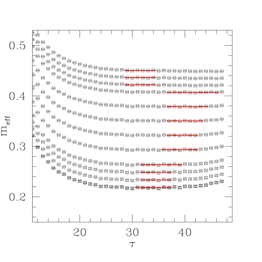
Figure 1: The effective mass plots for the pseudo-scalar meson made up of a quark and an anti-quark for zero three-momenta at $\beta=2.4$, $\nu=0.85$. With one quark mass parameter $m_{1}$ being fixed, different lines in the plot correspond to different values of the other quark mass $m_{2}$. The red horizontal bars in the plot indicates the ranges in which the mass of the meson are extracted.

The energy values of a pseudo-scalar meson with definite three-momentum ${\mathbf{k}}$ (including zero-momentum) is obtained from their respective correlation functions $C^{(PS)}({\mathbf{k}},t)$ by finding the plateaus in their effective mass plots. In Fig. 1, we show the effective mass plots of a pseudo-scalar meson with zero three-momentum for $\beta=2.4$, $\nu=0.85$. The pseudo-scalar meson consists of a quark and an anti-quark with all possible bare quark mass value combinations $(m_{1},m_{2})$. In Fig  1, we illustrate one of the situations with $m_{1}$ being fixed. The effective mass plots are shown for all $m_{2}$ values. Different lines in the plot then correspond to different values of the other bare quark mass parameter $m_{2}$. There are $12$ lines in each of these windows which correspond to $12$ different values of the bare quark mass $m_{2}$ being simulated. It is seen that all effective mass plots develop nice plateaus at large temporal separation and accurate values of the pseudo-scalar energy $E_{PS}(m_{1},m_{2},{\mathbf{k}})$ ( and also the mass $M_{PS}(m_{1},m_{2})=E_{PS}(m_{1},m_{2},{\mathbf{k}}=0)$ ) can thus be extracted. The red horizontal bars in the plot indicate the ranges in which the meson energy values are extracted. The errors for the data points in this plot are analyzed using the standard jack-knife method. The intervals from which we extract the energy values are self-adjusted according to the minimum of $\chi^{2}$ per degree of freedom. The quality of the effective mass plots for other parameter sets are similar.

3.2 Obtaining the pseudo-scalar meson energy at fixed quark masses

From the effective mass plots of pseudo-scalar meson correlation functions we obtain the energy values of a single pseudo-scalar meson with definite three-momentum ${\mathbf{k}}$: $E^{2}_{PS}(m_{1},m_{2},\nu,{\mathbf{k}})$. We thus have these energy values for each $\beta$, $\nu$, ${\mathbf{k}}$ and all possible bare quark mass values $(m_{1},m_{2})$ which we choose to calculate the meson correlation functions. Here the bare quark mass parameter is defined via:

$$m\equiv{1\over 2\kappa}-{1\over 2\kappa_{cr}(\nu)}\;.$$ (16)

where $\kappa_{cr}(\nu)$ is the critical hopping parameter at which the pion mass vanishes for a particular $(\beta,\nu)$. Note that this value depends on $\nu$ for a given $\beta$. For a given value of $\beta$, the critical hopping parameter $1/(2\kappa_{cr}(\nu)$ for each $\nu$ is obtained by fitting the pion (made up of equal mass quarks) mass squared versus $1/(2\kappa)$ using a quadratic function in the low quark mass region. From these fits, we obtain the critical value $1/(2\kappa_{cr}(\nu))$ for each $\nu$ at a given $\beta$.

The reason that we choose the bare quark mass parameter $m$ instead of the hopping parameter itself is the following. Our goal is to find the optimal values of $\nu$ such that the pseudo-scalar meson exhibits the proper dispersion relation in the low-momentum region. Therefore, for a given value of $\beta$, we want to fix the quark mass values and interpolate/extrapolate in $\nu$ to obtain the optimal value of $\nu$ at which the meson dispersion relation has the right form. This should be done for all possible quark mass values. It is better to perform this interpolation/extrapolation for fixed $m$ instead of fixed hopping parameter pair $\kappa$ since the critical hopping parameters themselves depend explicitly on $\nu$, as is seen evidently from the tree-level relation Eq. (6). This dependence is also seen from our simulation. So for different values of $\nu$, the same value of $\kappa$ for different $\nu$ in fact corresponds to different bare quark mass values. Therefore, it is more appropriate to interpolate/extrapolate in $\nu$ for fixed bare quark mass parameter pair $m$. Note that the bare quark mass $m$ as defined in (16) is an independent parameter of the quark action. In other words, no matter what the value of $1/(2\kappa_{cr}(\nu))$ comes out to be for each $\nu$, we could choose values of $m$, independent of $\nu$, since we are free to adjust the set of values for $\kappa$.

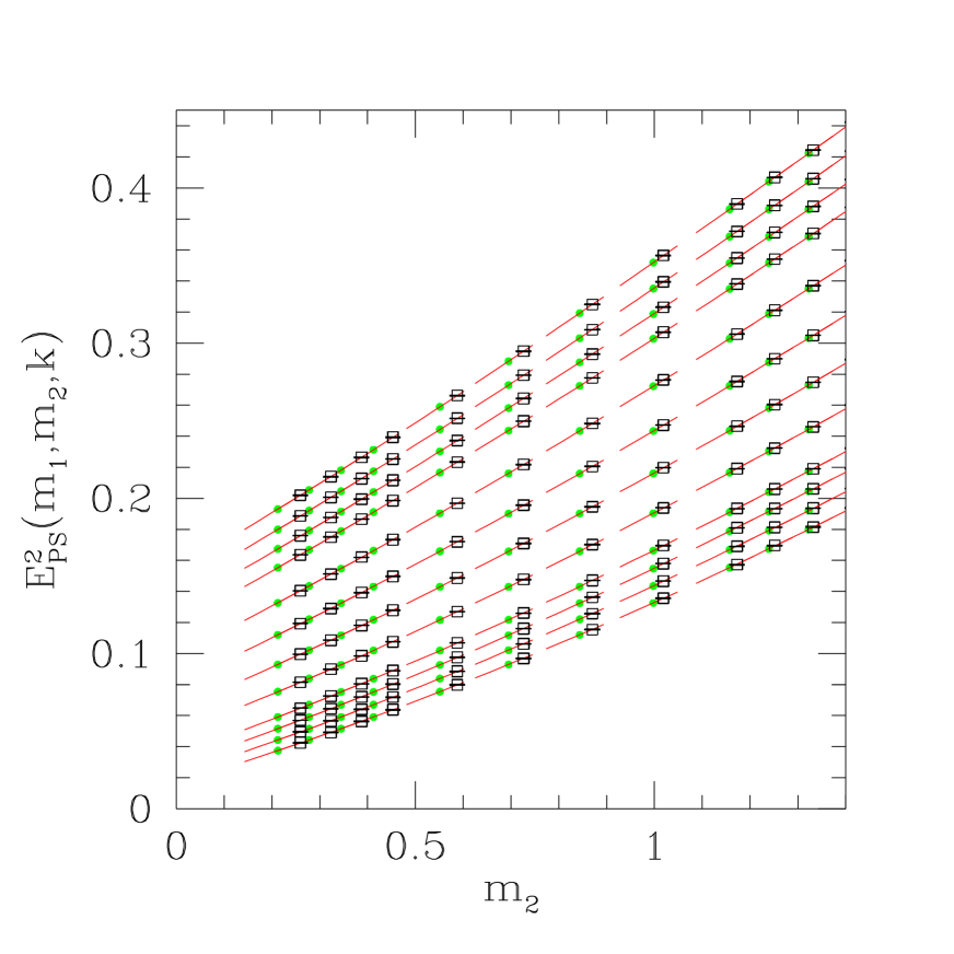
Figure 2: Interpolation of the pseudo-scalar meson energy squared $E^{2}_{PS}(m_{1},m_{2},\nu,{\mathbf{k}})$ versus the quark mass parameter pairs $(m_{1},m_{2})$ to the common values $(\bar{m}_{1},\bar{m}_{2})$ is shown for $\beta=2.4$, $\nu=0.85$. Only the zero three-momentum case is shown in this plot. Values of $E^{2}_{PS}(m_{1},m_{2},\nu,{\mathbf{k}}=0)$ are shown as data points. Red lines are the quadratic interpolations around each value of $\bar{m}$ using $6$ points of $m$ close to it.

It turns out that our choices of the hopping parameters for different $\nu$ are such that the range of $m$ are roughly the same for a given $\beta$ while the individual values are not identical. Therefore, before we make any interpolation/extrapolation in $\nu$, which should be done at fixed $m$ for all $\nu$, we first have to interpolate the energy values $E^{2}_{PS}(m_{1},m_{2},\nu,{\mathbf{k}})$ at different $\nu$ to the the same quark mass values: $(\bar{m}_{1},\bar{m}_{2})$. In the analysis, we pick the values of $\bar{m}$ to be the average of the three corresponding values at three different $\nu$. Of course, the choice of the common values for $\bar{m}$ at different $\nu$ is somewhat arbitrary and any other choice is equally well as long as the range of $\bar{m}$ roughly coincides with the ranges of the $m$ for different $\nu$ such that the interpolation can be done reliably. The interpolation of the energy values squared $E^{2}_{PS}(m_{1},m_{2},\nu,{\mathbf{k}})$ is performed by a quadratic interpolation in the quark mass parameter using 4-6 neighboring points close to the values of $\bar{m}$. It is checked that all interpolations yield good fitting qualities. In Fig. 2, we show this interpolation for $\beta=2.4$, $\nu=0.85$. Values of $E^{2}_{PS}(m_{1},m_{2},\nu,{\mathbf{k}})$ are shown as data points in the plot which correspond to zero three-momentum. The green points are the values of $\bar{m}$ to which $E^{2}_{PS}(m_{1},m_{2},\nu,{\mathbf{k}})$ are interpolated. Red line segments are the quadratic interpolation in the quark mass parameter using $4-6$ points around each value of $\bar{m}$. The number of points being taken in each interpolation is determined by the condition of minimum $\chi^{2}$ per degree of freedom. The situation for non-zero momentum is similar. All interpolation yields good fitting quality.

As the outcome of this procedure, we have all the quantities: $E^{2}_{PS}(\bar{m}_{1},\bar{m}_{2},\nu,{\mathbf{k}})$ that are at the same sequence of points $\bar{m}$ for different values of $\nu$. This procedure is performed for every value of $\beta$ and for every three-momentum mode under investigation (see Eq. (refeq:ns) for the momentum modes being studied). In the discussion below, we will drop the bars on the quark mass parameters for simplicity with the understanding that all energy levels $E_{PS}(m_{1},m_{2},\nu,{\mathbf{k}})$ are already interpolated to the same set of $(m_{1},m_{2})$ for different $\nu$.

3.3 Extraction of $Z$ parameter

In this work, we utilize lattices with asymmetric volumes. This asymmetry helps to break the cubic symmetry in the momentum space and lifts the degeneracy of the meson energies. For example, by using a lattice of size $6\times 9\times 12\times 50$, we have $8$ non-degenerate low-momentum modes, compared with only $4$ with symmetric volumes. This technique also proves to be useful for the measurement of other momentum-dependent quantities like the hadron-hadron scattering phase shifts [32, 33]. The three-momenta ${\mathbf{k}}$ in an asymmetric box of size $L_{1}\times L_{2}\times L_{3}$ are quantized according to:

$${\mathbf{k}}=\left({2\pi\over L_{1}}n_{1},{2\pi\over L_{2}}n_{2},{2\pi\over L_{3}}n_{3}\right)\;,$$ (17)

with ${\mathbf{n}}=(n_{1},n_{2},n_{3})\in\mathbb{Z}^{3}$ being three-dimensional integers. In this work, the energy values of a meson with the following $8$ three-momentum are measured:

$${\mathbf{n}} = (0,0,0)\;,(0,0,1)\;,(0,1,0)\;,(1,0,0)\;,$$ (18)

$$(0,1,1)\;,(1,0,1)\;,(1,1,0)\;,(1,1,1)\;.$$

For a given three-momentum ${\mathbf{k}}$, the pseudo-scalar meson energy levels $E^{2}_{PS}(m_{1},m_{2},\nu,{\mathbf{k}})$ are fitted according to the expected continuum dispersion relation:

$$E^{2}_{PS}(m_{1},m_{2},\nu,{\mathbf{k}})=M^{2}_{PS}(m_{1},m_{2},\nu)+Z_{PS}(m_{1},m_{2},\nu){\mathbf{k}}^{2}\;\;,$$ (19)

in the low-momentum region. The fitting is performed for pseudo-scalar mesons with all possible bare quark mass combinations: $(m_{1},m_{2})$. As a result of these fits, we obtain all the $Z$ parameters of the pseudo-scalar mesons as a function of two bare quark mass parameters: $Z_{PS}(m_{1},m_{2},\nu)$. In particular, for the pseudo-scalar meson made up of quarks with the same mass, the corresponding $Z$ parameter depends on one quark mass parameter, namely $Z_{PS}(m,m,\nu)$.

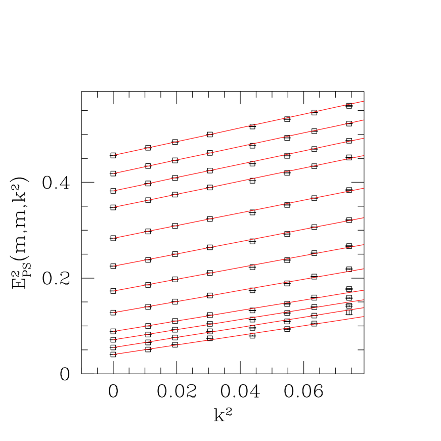
Figure 3: Dispersion relations of the pseudo-scalar meson at $\beta=2.4$, $0.85$. The data points show the pseudo-scalar meson energy squared $E^{2}_{PS}(m,m,\nu,{\mathbf{k}})$ at a given three-momentum ${\mathbf{k}}$ versus ${\mathbf{k}}^{2}$. The straight lines are the linear fits to the data with the fitting range starting from the low-momentum end and self-adjusted according to the minimum $\chi^{2}$ per degree of freedom. The slope of the lines then yield the desired $Z$ parameters. Different lines in the plot indicate the linear fits for different bare quark mass parameter $m$.

In Fig. 3, the linear fits of dispersion relations $E^{2}_{PS}(m,m,\nu,{\mathbf{k}}^{2})$ versus ${\mathbf{k}}^{2}$ for the pseudo-scalar meson with equal mass quark and anti-quark are shown for $\beta=2.4$, $\nu=0.85$. The straight lines in the plot represent the linear fits for $12$ values of bare quark parameter $m$. The linear fits utilize the low-momentum data points (including the zero-momentum point) according to Eq. (19) and the fitting range for each line is self-adjusted to yield the minimum $\chi^{2}$ for each degree of freedom. The slope of these lines then yield the parameters $Z_{PS}(m,m,\nu)$ for all bare quark mass parameter $m$. Fitting qualities for other $(\beta,\nu)$ are quite similar. We have also tried another (conventional) way of extracting the $Z$ parameters, namely by using only the zero-momentum point and the lowest non-vanishing momentum point (${\mathbf{n}}=(0,0,1)$ in this case). This is what has been done in the literature by many authors [12, 24, 25, 26]. We find that the $Z$ parameters are always better determined by using linear fits with more momentum points as compared with only two lowest momentum points. Therefore, we see the advantage of using asymmetric volumes for all our parameter sets.

3.4 Finding the optimal values of $\nu$

The optimal choice for the bare speed of light parameter $\nu$ in the quark action is determined from the corresponding pseudo-scalar meson dispersion relations, or more explicitly, from the $Z$ parameters $Z_{PS}(m,m,\nu)$ extracted from dispersion relations which is discussed the previous subsection. One requires that the dispersion relation of the pseudo-scalar meson made up of the same quark flavor reproduces its continuum counter-part in the low-momentum limit. That is to say, the optimal choice of $\nu$ has to be such that:

$$Z_{PS}[m,m,\nu_{opt}(m)]=1\;.$$ (20)

This yields the optimal value of $\nu$ as a function of the bare quark mass parameter: $\nu_{opt}(m)$.

In practice, we use the values of $Z_{PS}(m,m,\nu)$ at different $\nu$ and perform a linear extrapolation/interpolation in $\nu$ for every value of $m$.

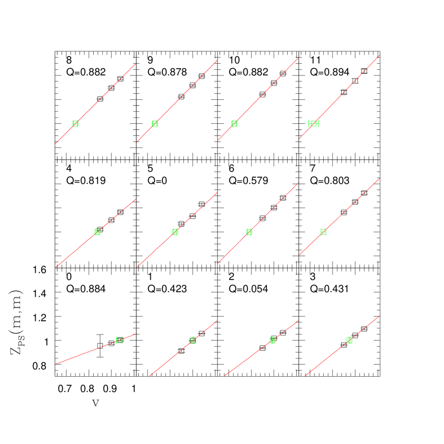
Figure 4: Determination of optimal speed of light parameter $\nu_{opt}(m)$ is shown for pseudo-scalar meson made of equal mass quark and anti-quark. Each small window corresponds to different values of bare quark mass parameter $m$. Data points in each window are the values of $Z_{PS}(m,m,\nu)$. They are fitted linearly versus $\nu$ and the optimal values of $\nu$ are determined by the condition: $Z_{PS}[m,m,\nu_{opt}(m)]=1$ for each given $m$. The results of $\nu_{opt}(m)$ are shown as green points in each window together with the corresponding error bar. In each window (corresponding to different $m$), the quality of the linear fit is also indicated.

This is shown in Fig 4 in the case of $\beta=2.4$. Each small window in this plot corresponds to different values of bare quark mass parameter $m$. Data points in each window are the values of $Z_{PS}(m,m,\nu)$ obtained from the pseudo-scalar dispersion relations. They are fitted linearly versus $\nu$ and the optimal values of $\nu$ are determined by the condition: $Z_{PS}[m,m,\nu_{opt}(m)]=1$. The results of $\nu_{opt}(m)$ for various $m$ are shown as green points together with the corresponding error bars. In each window (corresponding to different $m$), the quality of the linear fit is also shown.

3.5 Finding the physical bare quark mass parameters

Table 2: Extracted physical bare quark mass parameters for the charm and the strange quark and the optimal values for the bare speed of light parameter $\nu$ at physical quark masses for different $\beta$. Two sets of data (I) and (II) for $\beta=2.8$ corresponds to smaller ($6\cdot 9\cdot 12\cdot 50$) and larger ($8\cdot 12\cdot 16\cdot 50$) lattices, respectively.

$\beta$	$2.2$	$2.4$	$2.6$	$2.8(I)$	$2.8(II)$	$3.0$
$m^{(phy)}_{c}$	$1.879(2)$	$1.470(2)$	$1.194(1)$	$0.969(1)$	$0.978(5)$	$0.677(1)$
$m^{(phy)}_{s}$	$0.217(3)$	$0.163(1)$	$0.155(1)$	$0.120(2)$	$0.15(2)$	$0.073(2)$
$\nu_{opt}(m^{(phy)}_{c})$	$0.68(3)$	$0.71(3)$	$0.754(5)$	$0.75(1)$	$0.74(3)$	$0.84(1)$
$\nu_{opt}(m^{(phy)}_{s})$	$0.940(4)$	$0.933(3)$	$0.928(3)$	$0.98(2)$	$0.91(4)$	$0.99(1)$

For phenomenological reasons, one is particularly interested in the optimal parameters of $\nu$ near bare quark mass values that correspond to the physical interesting cases. In particular, we are interested in the values of $\nu_{opt}(m)$ at physical bare strange quark and bare charm quark mass, namely at $m=m^{(phy)}_{s}$ or $m=m^{(phy)}_{c}$. To find out this correspondence, one has to investigate the bare quark mass dependence of the meson mass and fix the bare quark mass parameter $m$ which corresponds to the physical case.

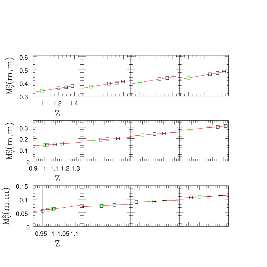
Figure 5: Linear extrapolations of $M^{2}_{V}(m,m,\nu)$ versus $Z_{PS}(m,m,\nu)$ for each value of $m$ at $\beta=2.4$. Different windows corresponds to different values of $m$. The linear extrapolations are shown by the straight lines in the windows.

To fix the physical bare quark mass parameters for the charm and the strange quark, we use the vector meson mass values. From the physical $J/\psi$ mass and the physical $\Phi$ meson mass, we can fix the bare quark mass parameters for the charm and the strange respectively. First, the vector meson mass squared at the optimal value of $\nu$: $M^{2}_{V}[m,m,\nu_{opt}(m)]$ is obtained by extrapolating to the optimal value of $\nu$. Once this quantity is at our disposal, we can perform extrapolation/interpolation in the bare quark mass $m$ to find out the physical bare quark mass for the charm and the strange quark. We therefore extrapolate $M^{2}_{V}(m,m,\nu)$ versus $Z_{PS}(m,m,\nu)$ linearly for each given value of $m$. The situation is shown in Fig 5 for $\beta=2.4$. Different small windows corresponds to different values of $m$. The linear extrapolations are shown by the straight lines in the windows. The extrapolated values of $M^{2}_{V}(m,m,\nu)$ at $Z_{PS}(m,m,\nu)=1$, then give the quantities $M^{2}_{V}[m,m,\nu_{opt}(m)]$. The results of $M^{2}_{V}[m,m,\nu_{opt}(m)]$ for all $m$ are then utilized in the quark mass interpolation/extrapolation.

In this work, we perform two quadratic fits for the meson mass versus the bare quark mass parameter $m$, one in the low quark mass region, the other in the heavy quark mass region. We always take the fitting form to be:

$$a^{2}_{t}M^{2}_{PS/V}[m,m,\nu_{opt}(m)]=A+Bm+Cm^{2}\;.$$ (21)

In all our cases, we find the fit parameter $A$ for the pseudo-scalar meson in the low quark mass region is always consistent with zero as it should be. In Fig. 6, we show this extrapolation for the vector meson mass at $\beta=2.4$.

Figure 6: Quadratic extrapolations of $M^{2}_{V}[m,m,\nu_{opt}(m)]$ versus the bare quark mass $m$ at $\beta=2.4$. The red line indicates a fit in the lower quark mass region. The green line is the corresponding fit in the heavy quark mass region. The corresponding fitting ranges are also shown in the figure. The fitting ranges are self-adjusted to yield minimum $\chi^{2}$ per degree of freedom. The blue horizontal line indicates the value for the physical $J/\psi$ meson while the pink horizontal line corresponds to the value of the physical $\Phi$ meson. The intersect with the green line and the red line then yields the estimate for $m^{(phy)}_{c}$ and $m^{(phy)}_{s}$, respectively.

The red line in the plot indicates a fit in the lower quark mass region. The green line is the corresponding fit in the heavy quark mass region. The corresponding fitting ranges are also shown in the figure. The fitting ranges are self-adjusted to yield minimum $\chi^{2}$ per degree of freedom. To obtain the physical charm quark mass parameter $m^{(phy)}_{c}$, we draw a horizontal line in this figure at the physical $J/\psi$ mass: $a^{2}_{t}M^{2}_{J/\psi}$. This is obtained by setting the scale using some physical quantity. In this work, we choose the hadronic scale $r_{0}=0.5$fm (the so-called Sommer scale) to set the physical scale. For different values of gauge coupling $\beta$, the values of $r_{0}/a_{s}$ are known from the literature [2, 3] which are also listed in Table 1 for reference. With this information, we know the physical meson masses in lattice unit. The blue horizontal line in the figure representing the value for physical $J/\psi$ intersects with the green line and the intersection point then yields the estimate for the physical charm quark mass parameter $m^{(phy)}_{c}$. Similarly, the pink horizontal line is at the value of physical $\Phi$ meson and the intersection point with the red line in the lower quark mass region yields the estimate for $m^{(phy)}_{s}$. The value of $m^{(phy)}_{c}$ and $m^{(phy)}_{s}$ thus obtained are listed in Table 2 for all $\beta$.

3.6 Optimal values of $\nu$ at physical quark mass parameters

After fixing the physical bare quark mass parameters for both the charm and the strange, we can obtain the optimal values of the speed of light parameter for these cases. In our notation, they correspond to $\nu_{opt}(m^{(phy)}_{c})$ and $\nu_{opt}(m^{(phy)}_{s})$, respectively. To get these values, we make interpolation/extrapolations of $\nu_{opt}(m)$ versus the bare quark mass parameter $m$ using quadratic functions in these parameters. We choose the appropriate range (heavy quark mass region and light quark mass region) for different cases.

In Fig 7 we show the extrapolation of $\nu_{opt}(m)$ versus $m$ in both the light and the heavy quark mass region at $\beta=2.4$. The red line is the quadratic fit to the data points in the low quark mass region while the green line is the fit in the heavy quark mass region. The final result of $\nu_{opt}(m^{(phy)}_{c})$ and $\nu_{opt}(m^{(phy)}_{s})$ are indicated by the blue and the pink solid point with errors at the position of the physical charm and strange quark mass respectively.

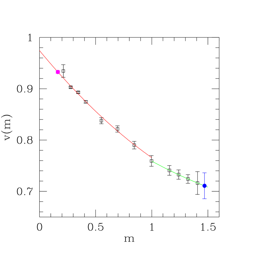
Figure 7: The result of $\nu_{opt}(m)$ is shown versus the bare quark mass $m$ for $\beta=2.4$. The red and the green line is a quadratic fit to the data points in the light and the heavy quark mass region respectively. At the position of the physical bare charm quark mass $m^{(phy)}_{c}$ and the physical bare strange quark mass $m^{(phy)}_{s}$, the result of $\nu_{opt}(m^{(phy)}_{c})$ and $\nu_{opt}(m^{(phy)}_{s})$ are shown by the blue and the pink solid point with errors, respectively.

The results for other values of $\beta$ are summarized in Table 2.

For the $\beta=2.8$ lattices, since the physical volume is somewhat small, one should check the size of finite size corrections. We therefore performed a low statistics run (about $120$ gauge field configurations) for this $\beta$. The final result is also tabulated in Table 2 labelled as $\beta=2.8(II)$. We see that the physical bare quark mass parameters changes, especially for the strange quark. However, the optimal value for the parameter $\nu$ at physical quark masses remain compatible within one or two standard deviations. Therefore, for the purpose of tuning the parameter $\nu$, this result seems to indicate that the finite size corrections are not large. Of course, if one would use the action to calculate physical quantities and compare with the experimental values, it would be safer to use larger volumes, which is what we will do in the future.

4 Conclusions

In this paper, we present a systematic numerical analysis on the tuning of the bare speed of light parameter $\nu$ in the tadpole improved anisotropic Wilson quark action. The tuning is done in a quark mass dependent way with quark mass values ranging from the strange to the charm. The optimal values of $\nu$ are obtained for various values of $\beta$ using the pseudo-scalar meson dispersion relations. With the help of the anisotropic lattices with asymmetric volumes, the dispersion relations can be measured with good accuracy. Using the tadpole improved anisotropic Wilson action with these optimized parameters, a quenched calculation can then be performed to study properties of hadrons made up of either light or heavy quarks. Therefore, with the same improved quark action one can study hadron spectrum and other physical properties in a wide range of quark masses. We hope to come to this issue in the near future.

References

- [1] C. Morningstar and M. Peardon. Phys. Rev. D, 56:4043, 1997.
- [2] C. Morningstar and M. Peardon. Phys. Rev. D, 60:034509, 1999.
- [3] C. Liu. Chinese Physics Letter, 18:187, 2001.
- [4] C. Liu. Communications in Theoretical Physics, 35:288, 2001.
- [5] C. Liu. In Proceedings of International Workshop on Nonperturbative Methods and Lattice QCD, page 57. World Scientific, Singapore, 2001.
- [6] C. Liu and J. P. Ma. In Proceedings of International Workshop on Nonperturbative Methods and Lattice QCD, page 65. World Scientific, Singapore, 2001.
- [7] C. Liu. Nucl. Phys. (Proc. Suppl.) B, 94:255, 2001.
- [8] A.X. El-Khadra, A.S. Kronfeld, and P.B. Mackenzie. Phys. Rev. D, 55:3933, 1997.
- [9] M. Alford, T. R. Klassen, and P. Lepage. Phys. Rev. D, 58:034503, 1998.
- [10] T. R. Klassen. Nucl. Phys. (Proc. Suppl.) B, 73:918, 1999.
- [11] J. Harada, A.S. Kronfeld, H. Matsufuru, N. Nakajima, and T. Onogi. Phys. Rev. D, 64:074501, 2001.
- [12] J. Harada, H. Matsufuru, T. Onogi, and A. Sugita. Phys. Rev. D, 66:014509, 2002.
- [13] P.B. Mackenzie, S.M. Ryan, and J.N. Simone. Nucl. Phys. (Proc. Suppl.) B, 63:305, 1998.
- [14] P. Chen. Phys. Rev. D, 64:034509, 2001.
- [15] R. Lewis, N. Mathur, and R.M. Woloshyn. Phys. Rev. D, 64:094509, 2001.
- [16] M. Okamoto et al. Phys. Rev. D, 65:094508, 2002.
- [17] A. Juettner and J. Rolf. Phys. Lett. B, 560:59, 2003.
- [18] Y. Nemoto, N. Nakajima, H. Matsufuru, and H. Suganuma. Phys. Rev. D, 68:094505, 2003.
- [19] C. Liu, J. Zhang, Y. Chen, and J.P. Ma. Nucl. Phys. B, 624:360, 2002.
- [20] G. Meng, C. Miao, X. Du, and C. Liu. hep-lat/0309048, 2003.
- [21] C. Miao, X. Du, G. Meng, and C. Liu. hep-lat/0403028, 2004.
- [22] X. Du, C. Miao, G. Meng, and C. Liu. hep-lat/0404017, 2004.
- [23] Junhua Zhang and C. Liu. Mod. Phys. Lett. A, 16:1841, 2001.
- [24] T. Umeda et al. Phys. Rev. D, 68:034503, 2003.
- [25] S. Hashimoto and M. Okamoto. Phys. Rev. D, 67:114503, 2003.
- [26] Justin Foley, Alan O Cais, Mike Peardon, and Sinead M. Ryan. hep-lat/0405030, 2004.
- [27] Junko Shigemitsu Stefan Groote. Phys. Rev. D, 62:014508, 2000.
- [28] H. Matsufuru, T. Onogi, and T. Umeda. Phys. Rev. D, 64:114503, 2001.
- [29] A. Frommer, S. Güsken, T. Lippert, B. Nöckel, and K. Schilling. Int. J. Mod. Phys. C, 6:627, 1995.
- [30] U. Glaessner, S. Guesken, T. Lippert, G. Ritzenhoefer, K. Schilling, and A. Frommer. hep-lat/9605008.
- [31] B. Jegerlehner. hep-lat/9612014.
- [32] X. Li and C. Liu. Phys. Lett. B, 587:100, 2004.
- [33] X. Feng, X. Li, and C. Liu. Phys. Rev. D, 70:014505, 2004.