Center Vortex Model for the Infrared Sector of $SU(3)$ Yang-Mills Theory – Vortex Free Energy

M. Quandt, H. Reinhardt^∗

Institut für Theoretische Physik, Universität Tübingen

D–72076 Tübingen, Germany.

M. Engelhardt

Physics Department, New Mexico State University

Las Cruces, NM 88003, USA

The vortex free energy is studied in the random vortex world-surface model of the infrared sector of $SU(3)$ Yang-Mills theory. The free energy of a center vortex extending into two spatial directions, which is introduced into Yang-Mills configurations when acting with the ’t Hooft loop operator, is verified to furnish an order parameter for the deconfinement phase transition. It is shown to exhibit a weak discontinuity at the critical temperature, corresponding to the weak first order character of the transition.

PACS: 12.38.Aw, 12.38.Mh, 12.40.-y
Keywords: Center vortices, infrared effective theory, ‘t Hooft loop, dual string tension

1 Introduction

Yang-Mills theory in four space-time dimensions undergoes a deconfinement phase transition at non-zero temperatures. One order parameter used in practice to characterize this transition is the Polyakov loop, which can be interpreted as representing a single static quark, immersed in a thermal Yang-Mills background. Since the confining phase is characterized by the free energy $F_{q}$ of such a quark being infinite, the Polyakov loop $\langle P\rangle=\exp(-F_{q})$ is expected to vanish below the critical temperature $T_{c}$ , while it should be non-zero in the deconfined (high temperature) phase. The Polyakov loop is closely related to the so-called center symmetry, which is broken at high temperatures $T>T_{c}$. Physically, this critical behavior is counterintuitive; usually, e.g. in most spin models, the high temperature phase is maximally symmetric and the symmetries are broken below the critical temperature. Furthermore, when formulated on a compact space with periodic boundary conditions (such as used in lattice calculations), Yang-Mills theory strictly speaking does not admit a single quark as a physical excitation, regardless of whether confinement is realized or not.

Not least due to these issues, it is instructive to consider an alternative dual (dis-)order parameter to characterize the deconfinement phase transition, namely the free energy associated with a center vortex world-surface. Center vortices are defined by the property that they contribute a center phase to a Wilson loop when piercing an area spanned by the latter. The center vortex free energy is expected to behave in a manner which is dual to the behavior of Wilson loops:

• The free energy of vortex world-surfaces extending into one space direction and the (Euclidean) time direction is expected to exhibit no area-law dependence on the vortex world-surface area at all temperatures $T$, if the corresponding dual (spatial) Wilson loops exhibit an area law for all $T$ (this is the case for pure $SU(N)$ Yang-Mills theory).

• The free energy of vortex world-surfaces extending into two spatial directions is expected to behave in a manner dual to the behavior of corresponding (temporal) Wilson loops: No area-law dependence of the free energy on the vortex world-surface area at temperatures below the deconfinement transition temperature $T_{c}$, but behavior according to an area law above the critical temperature.

The latter observation permits the definition of a (temperature-dependent) dual string tension $\tilde{\sigma}$ through the leading behavior of the excess free energy $F_{P}$ in the presence of asymptotically large vortex world-surfaces $P$,

$$F_{P}\equiv-\ln(Z_{P}/Z_{0})\,\,\longrightarrow\,\,\tilde{\sigma}(T)\,\mathrm{Area}(P)\,,\qquad T>T_{c}$$ (1)

which can serve as an order parameter for the deconfinement phase transition. Here, $Z_{0}$ denotes the conventional Yang-Mills partition function, whereas $Z_{P}$ denotes the partition function in the presence of the additional vortex $P$.

Using the vortex free energy as a confinement order parameter was first suggested by ‘t Hooft [1], who, initially working in the Schrödinger picture (using the Weyl gauge), defined a magnetic loop operator $\mathsf{M}(\mathscr{C})$ in the continuum [1] via equal-time commutation relations with all spatial Wilson loops $\mathsf{W}(\mathscr{C}^{\prime})$,

$$\mathsf{M}(\mathscr{C})\,\mathsf{W}(\mathscr{C}^{\prime})\,\mathsf{M}(\mathscr{C})^{\dagger}=z(\mathscr{C},\mathscr{C}^{\prime})\,\mathsf{W}(\mathscr{C}^{\prime})\,.$$ (2)

Here, $z(\mathscr{C},\mathscr{C}^{\prime})$ is an element of the center of the gauge group related to the integral linking number $\nu(\mathscr{C},\mathscr{C}^{\prime})$ of the two loops $\mathscr{C}$ and $\mathscr{C^{\prime}}$ in three space dimensions,

$$z(\mathscr{C},\mathscr{C}^{\prime})=\exp\left(i\frac{2\pi}{N}\,\nu(\mathscr{C},\mathscr{C}^{\prime})\right)\qquad\qquad(\,SU(N)\,\mbox{gauge group}\,).$$ (3)

The loop operator $\mathsf{M}$ of course is only defined implicitly by the commutation relation eq. (2). An explicit realization of this formal construction was recently derived and discussed in detail in ref. [2], cf. also [3]. Also in the dual language, the change of behavior of the vortex free energy across the deconfinement phase transition can be associated with a (magnetic) center symmetry [1, 4], which is broken in the low-temperature phase.

Subsequent to ‘t Hooft’s suggestion, realizations of the ‘t Hooft loop operator within the framework of lattice gauge theory formulated in 3+1-dimensional (Euclidean) space-time were discussed and schemes of measuring the free energies of the vortices thus introduced into the gauge configurations were devised [5, 6, 7, 8]. On this basis, sufficient conditions for confinement via vortex condensation were established [5, 9]. While the construction given in [5] admits the introduction of vortices of a large variety of shapes into gauge configurations (by imposing suitable boundary conditions on “vortex containers” within the lattice), in practice a particularly clean way to investigate the center vortex free energy is to consider specifically a vortex world-surface which occupies a complete two-dimensional plane in space-time. On a compact space-time, such as used in lattice Yang-Mills theory, such a world-surface is closed by virtue of the periodic boundary conditions; furthermore, its introduction corresponds to adopting twisted boundary conditions in the directions orthogonal to the vortex [10]. This is reflected in the fact that configurations with such a vortex are not connected to the conventional vacuum by the dynamics. The dynamics of Yang-Mills theory and also of the random vortex world-surface model considered in this work, cf. [11, 12], can create at most pairs of vortices occupying complete two-dimensional (parallel) planes in space-time; a single such vortex is topologically stable. Also, its free energy is not contaminated by ancillary effects such as the ones which occur, e.g., when one considers open vortex world-surfaces; these are bounded by center monopole world-lines, and their free energies thus contain additional contributions stemming from monopole self-energies and interactions, which need to be disentangled from the vortex free energy itself.

A number of measurements of vortex free energies have been carried out within lattice Yang-Mills theory, in a variety of guises. The excess free energy in the presence of twisted boundary conditions compared to periodic boundary conditions was evaluated in [13, 14, 15, 16, 17, 18, 19, 20, 21]. Also the free energy of more varied vortex configurations, including open vortex world-surfaces [8, 17, 22, 23] and intersecting planar vortices [18] was investigated. Partition functions in the presence of twists can furthermore be related to electric flux free energies via $Z(N)$ Fourier transforms [10]; a thorough discussion of this together with detailed measurements can be found in [18], cf. also [24, 25] for earlier work with this focus. In addition, in the case of a system with a first order deconfinement transition, as found, e.g., for $SU(3)$ color, the vortex free energy in the deconfined phase is related to the $Z(3)$ order-order interface tension [3]; for an evaluation of this interface tension using a different method, cf. [26]. With auxiliary information about wetting properties [26, 27], the order-order interface tension can in turn be connected to the order-disorder interface tension at the critical temperature. Direct measurements of the order-disorder interface tension at the $SU(3)$ deconfinement transition were reported in [27, 28, 29, 30, 31, 32, 33, 34]; for a recent comparison with data obtained using a new calculational method based on the vortex free energy, cf. [21]. The results obtained in the present work will be put in relation to the survey presented in [21] in section 4.

2 Vortex free energy in the random vortex world-surface model

The main purpose of the work presented here is to compute the dual string tension $\tilde{\sigma}(T)$ by evaluating the free energy of appropriate vortex world-surfaces within the $SU(3)$ random vortex world-surface model. This model was first defined and studied for the gauge group $SU(2)$ in refs. [11, 35] and later extended to the $SU(3)$ case in refs. [12, 36]. It describes the infrared sector of Yang-Mills theory as an ensemble of random (thick) center vortex world-surfaces. On a space-time lattice dual to the one Yang-Mills lattice links are defined on, the vortex world-surfaces are composed of elementary squares, and can thus link with the Wilson loops of the original lattice. As described and motivated in detail in [11, 12], since the model is not intended to describe the structure of the theory at arbitarily short distances, it has a fixed lattice spacing $a$ representing the vortex thickness. Continuity of the magnetic flux forces the vortex world-surfaces to be closed, and the statistical weight of a (closed) vortex world-surface is determined by a model action inspired by a gradient expansion of the Yang-Mills action of a center vortex [37]:

$$S = \epsilon\sum_{x}\sum_{\mu,\nu\atop\mu<\nu}|q_{\mu\nu}(x)|+c\sum_{x}\sum_{\mu}\Bigg{[}\sum_{\nu<\lambda\atop\nu\neq\mu,\lambda\neq\mu}\Big{(}|q_{\mu\nu}(x)\,q_{\mu\lambda}(x)|+|q_{\mu\nu}(x)\,q_{\mu\lambda}(x-e_{\lambda})|+$$ (4)

$$\qquad\qquad\qquad\qquad+|q_{\mu\nu}(x-e_{\nu})\,q_{\mu\lambda}(x)|+|q_{\mu\nu}(x-e_{\nu})\,q_{\mu\lambda}(x-e_{\lambda})|\Big{)}\Bigg{]}$$

Here, the (dual) lattice elementary square extending from the dual lattice site $x$ into the positive $\mu$ and $\nu$ directions is associated with a triality $q_{\mu\nu}(x)\in\{-1,0,1\}$ (in the case of an underlying $SU(3)$ gauge group), labeling the center flux carried by that elementary square. The value $q_{\mu\nu}(x)=0$ indicates that the square is not part of a vortex world-surface, whereas the other two values are associated with the two types of center flux a vortex surface can carry. The two terms in eq. (4) correspond to a Nambu-Goto and a curvature term, respectively. They implement the notion that vortices, on the one hand, may be associated with a surface tension such that it costs a certain action increment $\epsilon$ to add an elementary square to the surface. On the other hand, vortices are stiff, such that an action increment $c$ is incurred for each pair of elementary squares in the vortex surface which share a link but do not lie in the same plane (i.e., vortex curvature is penalised). For details on the physical foundations of the model, and the determination of the couplings $\epsilon$ and $c$, the reader is referred to refs. [11, 12]. In practice, physical ensembles which reproduce the gross features of the corresponding Yang-Mills theory in the infrared can be achieved with $\epsilon=0$. In the case of an underlying $SU(2)$ gauge group, the value $c=0.24$ generates a physical ensemble, whereas in the case of the $SU(3)$ gauge group, the appropriate value is $c=0.21$. These values were determined by requiring the models to correctly reproduce the ratio of the deconfinement temperature $T_{c}$ to the square root of the zero-temperature string tension $\sqrt{\sigma}$ found in the corresponding Yang-Mills theory.

Since the random vortex world-surface model was proposed as an effective description of the long-range properties of Yang-Mills theory, including its deconfinement phase transition, the temperature dependence of $\tilde{\sigma}(T)$ near the transition is a non-trivial and important test of the model. In the random vortex world-surface model, the elementary squares $q_{\mu\nu}(x)$ of the dual lattice represent the building blocks for the dynamical center vortex degrees of freedom; in this framework, it is thus particularly simple to introduce an additional vortex world-surface into the configurations. One simply needs to replace

$$q_{\mu\nu}(x)\longrightarrow(q_{\mu\nu}(x)+\bar{q})\,\mbox{mod}\,3$$ (5)

for all elementary squares $q_{\mu\nu}(x)$ making up the world-surface in question, with a fixed value of $\bar{q}\in\{-1,1\}$. The two possible values of $\bar{q}$ are related by a space-time inversion which reverses the direction of magnetic flux (and leaves the action invariant); one can therefore restrict oneself to $\bar{q}=1$ without loss of generality.

The dual string tension is obtained in this work specifically by calculating the excess free energy in the presence of a vortex world-surface $P$ occupying an entire lattice plane extending into two spatial directions. The plane $P$ is composed of elementary squares $p_{i}$ with $1\leq i\leq I$, where $I$ is the number of elementary squares in $P$. Let $Q$ denote collectively a vortex world-surface configuration $\{q_{\mu\nu}(x)\}$, and $S[Q]$ the corresponding action (4). It will be useful for the following to introduce a notation for introducing additional elementary vortex squares $p_{i}$ into configurations; this is best done recursively: Starting with a configuration $Q_{0}$ from the conventional random vortex world-surface ensemble, without any additional vortex surfaces introduced, define the configuration $Q_{i}$ as the configuration obtained by effecting the transformation (5) specifically on the elementary square $p_{i}$ of the configuration $Q_{i-1}$. One can also define corresponding partition functions $Z_{i}$ as

$$Z_{i}=\int[dQ_{i}]\exp(-S[Q_{i}])=\int[dQ_{0}]\exp(-S[Q_{i}])\ .$$ (6)

In the notation of eq. (1), $Z_{P}\equiv Z_{I}$. To obtain the dual string tension, it is thus necessary to evaluate

$$\frac{Z_{I}}{Z_{0}}=\frac{\int[dQ_{0}]\exp(-S[Q_{0}])\exp(-(S[Q_{I}]-S[Q_{0}]))}{\int[dQ_{0}]\exp(-S[Q_{0}])}\equiv\left\langle\exp(-(S[Q_{I}]-S[Q_{0}]))\right\rangle_{0}\ .$$ (7)

However, this expression is of little practical use as it suffers from a serious overlap problem: The quantity being averaged varies over many orders of magnitude, so that most configurations only give an exponentially small contribution to the average. The resulting numerical noise precludes extracting a useful signal. This problem is addressed by using an algorithm introduced by de Forcrand et al [17]. By decomposing

$$\frac{Z_{I}}{Z_{0}}=\frac{Z_{I}}{Z_{I-1}}\cdot\frac{Z_{I-1}}{Z_{I-2}}\cdots\frac{Z_{1}}{Z_{0}}\ ,$$ (8)

the problem is separated into the calculation of a (sizeable) number of independent expectation values with good overlap; namely, one evaluates the effect of introducing just one additional elementary square $p_{i}$ into the configurations at a time,

$$\frac{Z_{i}}{Z_{i-1}}=\frac{\int[dQ_{0}]\exp(-S[Q_{i-1}])\exp(-(S[Q_{i}]-S[Q_{i-1}]))}{\int[dQ_{0}]\exp(-S[Q_{i-1}])}\equiv\left\langle\exp(-(S[Q_{i}]-S[Q_{i-1}]))\right\rangle_{i-1}\ .$$ (9)

Note that the classes of configurations $Q_{i}$, excepting $Q_{0}$ and $Q_{I}$, contain open vortex world-surfaces, bounded by center monopoles, which violate the Bianchi identity. As already discussed further above, these are unphysical objects which are introduced here merely as intermediate mathematical constructs. If one implemented the Bianchi constraint in terms of an infinite action term penalizing center monopoles, all intermediate partition functions $Z_{i}$ (apart from $Z_{0}$ and $Z_{I}$) strictly speaking would vanish. These $Z_{i}$ thus really are calculated with a modified weight in which the infinite self-energies of the center monopoles introduced explicitly into the configurations are left out (all other center monopoles are of course still completely suppressed; the integration $\int[dQ_{0}]$ is over the conventional ensemble which respects the Bianchi identity). Of course, the final result for the dual string tension ultimately depends only on the physical partition functions $Z_{I}$ and $Z_{0}$; all intermediate partition functions cancel out in the product (8).

In practice, it is possible to improve the measurement of the individual expectation values (9) further by using a multi-hit procedure. The quantity $S[Q_{i}]-S[Q_{i-1}]$ depends only on the configuration in the neighborhood of the elementary square $p_{i}$; thus, by performing multiple configuration updates and measurements in that neighborhood before carrying out the next global update of the configuration, statistics can be improved considerably without spoiling detailed balance or ergodicity.

As the plane $P$ is filled up one elementary square $p_{i}$ at a time, one can record the free energies

$$F_{i}=-\ln(Z_{i}/Z_{0})$$ (10)

of the partial vortex surfaces, up to the free energy $F_{I}$ of the full plane $P$. The dual string tension is extracted as

$$\tilde{\sigma}(T)=\frac{F_{I}}{Ia^{2}}$$ (11)

where $a$ denotes the lattice spacing. As already mentioned above, the lattice spacing in the random vortex world-surface model is a fixed physical quantity related to the transverse thickness of the vortices; for a detailed discussion, cf. [11, 12]. At the physical point $\epsilon=0,c=0.21$ of the $SU(3)$ model, its value is $a=0.39\,\mbox{fm}$, where the scale was fixed by equating the zero-temperature string tension with $(440\,\mbox{MeV})^{2}$. Besides the dual string tension, which is the principal quantity of interest in this work, below also the partial free energies $F_{i}$ will be discussed.

3 Numerical results

3.1 General remarks

Since the lattice spacing $a$ of the random vortex world-surface model is taken to be a fixed quantity that is not scaled towards a continuum limit, the temperature in the model can only be changed in rather large steps if the coupling constants are kept fixed. However, by employing an interpolation method, a continuous range of temperatures can be explored [11, 12]: For all measurements in this work, $\epsilon=0$ is fixed and only variations in the curvature coupling $c$ are considered. For several temporal extensions $N_{0}=1,2,3$ of the lattice, one can vary the coupling $c$ until the deconfinement phase transition is observed at critical couplings $c_{i}^{\ast}\equiv c^{\ast}(N_{0}=i)$. The critical couplings for the gauge group $SU(3)$ on lattices of extension $N_{0}\times 30^{3}$ are

$$N_{0}=i$$ 1 2 3

0.0872 0.2359 0.335

From the critical temperature $aT_{c}=1/N_{0}$ for the three values $c=c_{i}^{\ast}$, the function $a\,T_{c}(c)$ can be determined for all relevant couplings $c$ by interpolation. This, in turn, specifies the temperature in units of the deconfinement transition temperature for any $c$ and $N_{0}$ via

$$\frac{T}{T_{c}}=\frac{1}{N_{0}\cdot aT_{c}(c)}\,.$$

In particular, this permits carrying out measurements at a given $T/T_{c}$ for different $N_{0}$ and the corresponding $c$. Combining these measurements, the quantity in question, at the given $T/T_{c}$, can then also be obtained for the physical value $c=0.21$ by interpolation in $c$. This procedure is used to arrive at the last two columns of Table 1 below.

To be consistent with this determination of the temperature, and also in order to minimize finite-size effects, the evaluation of the dual string tension in this work was likewise carried out on $N_{0}\times 30^{3}$ lattices. To check for finite-size effects, control measurements were performed on lattices with spatial extensions of $10$, $12$ and $16$ lattice spacings; in all cases, the discrepancies between measurements of the dual string tension at spatial extensions $16$ and $30$, respectively, were smaller than the statistical errors of the measurements.

3.2 Boundary effects on open vortex world-surfaces

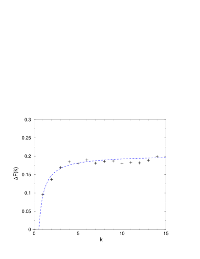
Figure 1: Left panel: Free energies $F_{i}$, cf. eq. (10), of partial vortex world-surfaces, as a function of the number $i$ of elementary squares included in the surface. Measurements were taken on a $30^{3}\times 2$ lattice at $\epsilon=0$ and $c=0.2550$, which corresponds to $T/T_{c}$ = 1.093 (deconfined phase). Right panel: The residual magnetic monopole correlation $\Delta F(k)=F_{kN_{s}}-F_{I}\cdot kN_{s}/I$ as a function of the monopole pair separation in lattice units $k$, from the same measurement. The curve represents a fit by a (self-energy) constant plus a Yukawa potential, $\Delta F(k)=V_{0}+\exp(-\mu k)/k$.

The left-hand panel of Fig. 1 shows a typical result for the free energies $F_{i}$ of partial vortex world-surfaces in the deconfined phase, at $T/T_{c}=1.093$. The area of the surfaces in units of $a^{2}$ is $i$, and the approximate linear rise with $i$ thus indicates an area law, as expected in the deconfined phase. However, there are also systematic deviations from a behavior purely proportional to the area, in particular for small $i$, and for large $i$, when the surface almost completely covers the lattice plane it is located in.

These deviations can be formally attributed to self-energies and residual interactions of the center monopole world-lines which necessarily bound the intermediate open vortex world-surfaces. They are the most transparent when considering surfaces made up of full rows of elementary squares, i.e., when $i$ is an integer multiple of the spatial extension of the lattice, $i=kN_{s}$. In this case, there are two parallel center monopole world-lines winding along a spatial dimension of the lattice at a distance $k\cdot a$ and the deviations from the area law formally correspond to self-energies and residual interactions of the two monopoles. The right-hand panel in Fig. 1 displays the deviation $\Delta F(k)=F_{kN_{s}}-F_{I}\cdot kN_{s}/I$ from an area law as a function of the center monopole separation in lattice units $k$. It should again be noted that this quantity does not have an immediate physical interpretation. Apart from the monopoles propagating into a spatial instead of the temporal direction, they strictly speaking are associated with an infinite self-energy preventing their appearance in the physical vortex ensemble. An additional finite contribution to this infinite self-energy is physically inconsequential.

3.3 The dual string tension

Approaching the deconfinement phase transition temperature $T_{c}$ from below, one can verify that the dual string tension is compatible with zero. Corresponding measurements on $30^{3}\times 2$ lattices at couplings $c$ below the critical coupling $c=0.2359$, which realize the confining phase, yield:

$$c$$

0.21

0.23

0.235

Also, for comparison, a measurement on a $16^{3}\times 2$ lattice at $c=0.21$ resulted in $\tilde{\sigma}\,a^{2}=-0.000205\pm 0.000271$.

Above the phase transition temperature, measurements were carried out for a sequence of temperatures $T/T_{c}$. As displayed in Table 1, for each temperature, measurements were performed both on a $30^{3}\times 2$ and a $30^{3}\times 1$ lattice with the appropriate couplings $c$ realizing the given temperature. Thus, for a fixed temperature $T/T_{c}$, the dual string tension $\tilde{\sigma}$ for the two values $c_{1}$ ($N_{0}=1$) and $c_{2}$ ($N_{0}=2$) is obtained. To arrive at the physical value, those two results are then interpolated linearly to the physical coupling $c_{\rm phys}=0.21$. Since the lattice spacing at the physical point is known in absolute units, the physical value of the dual string tension can also be given in absolute units. This is shown in the last column of Table 1. These results are also presented graphically in Fig. 2.

$T/T_{c}$ $c$ $\tilde{\sigma}\,(30a)^{2}$ $\tilde{\sigma}_{\rm phys}\,(30a)^{2}$ $\sqrt{\tilde{\sigma}_{\rm phys}}$ / MeV $N_{0}=1$ 0.08753 4.9 1.0015 $N_{0}=2$ 0.2362 6.6 6.3 42.3 $N_{0}=1$ 0.0884 14.4 1.0052 $N_{0}=2$ 0.2370 10.8 11.5 57.1 $N_{0}=1$ 0.0899 29.3 1.0118 $N_{0}=2$ 0.2384 25.5 26.2 86.2 $N_{0}=1$ 0.0905 35.6 1.0147 $N_{0}=2$ 0.2390 28.7 30.0 92.2 $N_{0}=1$ 0.0916 46.7 1.0195 $N_{0}=2$ 0.2400 30.0 33.4 97.3 $N_{0}=1$ 0.0969 98.1 1.044 $N_{0}=2$ 0.2450 57.3 66.9 138 $N_{0}=1$ 0.1021 144 1.068 $N_{0}=2$ 0.2500 80.2 97.5 166 $N_{0}=1$ 0.1073 188 1.093 $N_{0}=2$ 0.2550 110 134 195 $N_{0}=1$ 0.1123 226 1.118 $N_{0}=2$ 0.2600 133 164 216 $N_{0}=1$ 0.1495 437 1.326 $N_{0}=2$ 0.3000 308 385 330 $N_{0}=1$ 0.1756 513 1.500 $N_{0}=2$ 0.3350 387 486 371 $N_{0}=1$ 0.1929 548 1.629 $N_{0}=2$ 0.4500 435 540 391 $N_{0}=1$ 0.2100 579 1.770 $N_{0}=2$ — — 579 405

Table 1: Dual string tension $\tilde{\sigma}$ measured on $30^{3}\times N_{0}$ lattices with $\epsilon=0$. The curvature couplings $c$ were chosen such that the corresponding measurements for $N_{0}=1$ and $N_{0}=2$ implement the same temperature $T/T_{c}$. The results in the last two columns represent the interpolation to the physical value $c=0.21$. Since the lattice spacing at this point is fixed to $a=0.39\,\mathrm{fm}$, the value of the physical dual string tension $\tilde{\sigma}_{\rm phys}$ can be given in absolute numbers.

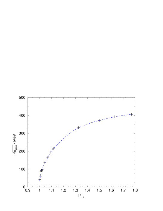
Figure 2: Dual string tension $\tilde{\sigma}$ as a function of the temperature $T$ in the deconfined phase, taken from Table 1.

As can be seen from the data, the dual string tension $\tilde{\sigma}$ rises with increasing temperature in the deconfined phase. As the phase transition is approached from above, the dual string tension $\tilde{\sigma}$ quickly vanishes as is expected for an order parameter. Since the phase transition in the $SU(3)$ case is weakly first order [12], a weak discontinuity is expected in the dual string tension $\tilde{\sigma}(T)$. The discontinuity can be obtained by using the two data points nearest to $T_{c}$ and extrapolating linearly to $T=T_{c}$. The statistical uncertainty for the dimensionless combination $\tilde{\sigma}_{\rm phys}\,(30a)^{2}$ (the second to last column in Tab. 1) is $6.3\pm 0.4$ at $T/T_{c}=1.0015$ and $11.5\pm 0.5$ at $T/T_{c}=1.0052$. Varying the slope of the extrapolation line within these error bounds, the resulting value at $T=T_{c}+$ is

$$\left.\sqrt{\tilde{\sigma}_{\rm phys}}\right|_{T=T_{c}+}=(34.5\pm 3.3)\,\mathrm{MeV}\,.$$ (12)

As a cross-check, a spline extrapolation through the five data points nearest to the transition (up to $T/T_{c}=1.0195$) yields $\sqrt{\tilde{\sigma}_{\rm phys}}|_{T=T_{c}+}\approx 36.8\,\mathrm{MeV}$, whereas using only the three nearest data points leads to $\sqrt{\tilde{\sigma}_{\rm phys}}|_{T=T_{c}+}\approx 36.5\,\mathrm{MeV}$, both consistent with (12). Also, linear regression through the nearest three data points yields $\sqrt{\tilde{\sigma}_{\rm phys}}|_{T=T_{c}+}\approx 35.5\,\mathrm{MeV}$. The data thus provide a clear signal for the discontinuity of the dual string tension $\tilde{\sigma}$ at $T=T_{c}$, in accordance with the first order character of the phase transition previously verified for the $SU(3)$ random vortex world-surface model via the action density distribution at the critical temperature [12]. The small value of the discontinuity compared with typical strong interaction scales again demonstrates the weak first order character of the transition.

4 Discussion

The dual string tension in the framework of the $SU(3)$ random vortex world-surface model was verified in this investigation to represent an order parameter for the deconfinement phase transition, and to furthermore reflect the weak first order character of the transition. Quantitatively, the result (12) for the discontinuity at the transition,

$$\left.\sqrt{\tilde{\sigma}}\right|_{T=T_{c}+}=(34.5\pm 3.3)\,\mathrm{MeV}\,,$$

is smaller than one would expect from measurements of the order-disorder interface tension in $SU(3)$ lattice Yang-Mills theory assuming perfect wetting. The available data for the order-disorder tension [21] indicate a value of $\sigma_{od}\approx 0.015\,T_{c}^{2}$, which translates to $\sigma_{od}\approx(34\,\mbox{MeV})^{2}$, if the scale is set by equating the zero-temperature string tension with $(440\,\mbox{MeV})^{2}$. Assuming perfect wetting, the order-order interface tension, equivalent to the dual string tension, would be expected to take the value $2\sigma_{od}\approx(48\,\mbox{MeV})^{2}$.

There are, however, caveats to this comparison. On the one hand, though wetting has been observed in $SU(3)$ lattice Yang-Mills theory [26, 27], there remains an uncertainty as to its quantitative extent. On the other hand, there are also still significant uncertainties involved in extrapolating the aforementioned measurements of the order-disorder tension from the lattice spacings they were obtained at to the continuum limit. Current efforts to accurately determine the dual string tension at the deconfinement transition in $SU(3)$ lattice Yang-Mills theory [21] actually indicate significantly higher values of the tension at coarse lattice spacings; however, also in this case, no conclusive statement concerning the extrapolation to the continuum limit can be made on the basis of the preliminary data presently available. These data display a substantial downward trend for the dual string tension as the lattice spacing is reduced.

In view of the current status, it seems premature to draw a final conclusion as to whether the result obtained here within the random vortex world-surface model quantitatively reflects the behavior of full $SU(3)$ Yang-Mills theory or not. On the other hand, it should be noted that it is possible to significantly enhance the first-order character of the deconfinement phase transition in the vortex model by introducing an additional term into the action (4) which favors vortex branchings; the latter are presumably instrumental in establishing first-order behavior, since they represent the feature which qualitatively distinguishes $SU(3)$ vortex configurations from $SU(2)$ vortex configurations. Introducing such a mechanism has indeed proven to be efficacious in preliminary investigations of the $SU(4)$ random vortex world-surface model, which will be reported in a separate publication. Whether it will ultimately be necessary to invoke this type of mechanism in the $SU(3)$ case is as yet unclear in view of the current status of the data discussed above; however, in the $SU(4)$ case, such an additional term in the action will certainly play a role.

References

- [1] G. ’t Hooft, Nucl. Phys. B138 (1978) 1.
- [2] H. Reinhardt, Phys. Lett. B557 (2003) 317.
- [3] C. Korthals-Altes, A. Kovner and M. A. Stephanov, Phys. Lett. B469 (1999) 205.
- [4] C. Korthals-Altes and A. Kovner, Phys. Rev. D 62 (2000) 096008.
-
[5]
G. Mack and V. B. Petkova, Ann. Phys. (NY) 123
(1979) 442;
G. Mack and V. B. Petkova, Ann. Phys. (NY) 125 (1980) 117. - [6] A. Ukawa, P. Windey and A. H. Guth, Phys. Rev. D21 (1980) 1013.
- [7] E. T. Tomboulis, Phys. Rev. D 23 (1981) 2371.
- [8] L. Del Debbio, A. Di Giacomo and B. Lucini, Nucl. Phys. B594 (2001) 287.
- [9] T. G. Kovacs and E. T. Tomboulis, Phys. Rev. D 65 (2002) 074501.
- [10] G. ’t Hooft, Nucl. Phys. B153 (1979) 141.
- [11] M. Engelhardt and H. Reinhardt, Nucl. Phys. B585 (2000) 591.
- [12] M. Engelhardt, M. Quandt, H. Reinhardt, Nucl. Phys. B685 (2004) 227.
-
[13]
G. Mack and E. Pietarinen, Phys. Lett. B94
(1980) 397;
G. Mack and E. Pietarinen, Nucl. Phys. B205 [FS5] (1982) 141. - [14] K. Kajantie, L. Kärkkäinen and K. Rummukainen, Nucl. Phys. B357 (1991) 693.
-
[15]
T. G. Kovacs and E. T. Tomboulis,
Nucl. Phys. Proc. Suppl. 83 (2000) 553;
T. G. Kovacs and E. T. Tomboulis, Phys. Rev. Lett. 85 (2000) 704. - [16] A. Hart, B. Lucini, Z. Schram and M. Teper, JHEP 0006 (2000) 040.
-
[17]
P. de Forcrand, M. D’Elia and M. Pepe,
Phys. Rev. Lett. 86 (2001) 1438;
P. de Forcrand, M. D’Elia and M. Pepe, Nucl. Phys. Proc. Suppl. 94 (2001) 494. -
[18]
P. de Forcrand and L. von Smekal, Phys. Rev. D66
(2002) 011504;
P. de Forcrand and L. von Smekal, Nucl. Phys. Proc. Suppl. 106 (2002) 619. - [19] L. von Smekal and P. de Forcrand, Nucl. Phys. Proc. Suppl. 119 (2003) 655.
- [20] P. de Forcrand and O. Jahn, Nucl. Phys. Proc. Suppl. 119 (2003) 649.
- [21] P. de Forcrand, B. Lucini and M. Vettorazzo, hep-lat/0409148.
-
[22]
C. Hoelbling, C. Rebbi and V. A. Rubakov,
Nucl. Phys. Proc. Suppl. 73 (1999) 527;
C. Hoelbling, C. Rebbi and V. A. Rubakov, Nucl. Phys. Proc. Suppl. 83 (2000) 485;
C. Hoelbling, C. Rebbi and V. A. Rubakov, Phys. Rev. D 63 (2001) 034506. - [23] L. Del Debbio, A. Di Giacomo and B. Lucini, Phys. Lett. B500 (2001) 326.
- [24] A. Hasenfratz, P. Hasenfratz and F. Niedermayer, Nucl. Phys. B329 (1990) 739.
- [25] A. González-Arroyo and P. Martínez, Nucl. Phys. B459 (1996) 337.
- [26] R. Brower, S. Huang, J. Potvin, C. Rebbi and J. Ross, Phys. Rev. D 46 (1992) 4736.
- [27] B. Grossmann, M. L. Laursen, T. Trappenberg and U.-J. Wiese, Nucl. Phys. B396 (1993) 584.
- [28] K. Kajantie, L. Kärkkäinen and K. Rummukainen, Nucl. Phys. B333 (1990) 100.
- [29] R. Brower, S. Huang, J. Potvin and C. Rebbi, Phys. Rev. D 46 (1992) 2703.
-
[30]
B. Grossmann, M. L. Laursen, T. Trappenberg and U.-J. Wiese,
Nucl. Phys. Proc. Suppl. 30 (1993) 869;
B. Grossmann and M. L. Laursen, Nucl. Phys. B408 (1993) 637. - [31] Y. Iwasaki, K. Kanaya, L. Kärkkäinen, K. Rummukainen and T. Yoshie, Phys. Rev. D 49 (1994) 3540.
- [32] Y. Aoki and K. Kanaya, Phys. Rev. D 50 (1994) 6921.
- [33] B. Beinlich, F. Karsch and A. Peikert, Phys. Lett. B390 (1997) 268.
- [34] A. Papa, Phys. Lett. B420 (1998) 91.
-
[35]
M. Engelhardt, Nucl. Phys. B585 (2000) 614;
M. Engelhardt, Nucl. Phys. B638 (2002) 81. - [36] M. Engelhardt, Phys. Rev. D 70 (2004) 074004.
- [37] M. Engelhardt and H. Reinhardt, Nucl. Phys. B567 (2000) 249.