The speed of sound and specific heat in the QCD plasma:
hydrodynamics, fluctuations and conformal symmetry

Abstract

We report the continuum limits of the speed of sound, $C_{s}$, and the specific heat at constant volume, $C_{\scriptscriptstyle V}$, in quenched QCD at temperatures of $2T_{c}$ and $3T_{c}$. At these temperatures, $C_{s}$ is within 2-$\sigma$ of the ideal gas value, whereas $C_{\scriptscriptstyle V}$ differs significantly from the ideal gas. However, both are compatible with results expected in a theory with conformal symmetry. We investigate effective measures of conformal symmetry in the high temperature phase of QCD.

I Introduction

It is now a well-established fact that the pressure, $P$, and the energy density, $\epsilon$, deviate boyd in the high temperature phase of QCD by about 25% from their ideal gas values at a temperature of about $3T_{c}$, where $T_{c}$ is the transition temperature. Early expectations that $\epsilon$ would count the number of degrees of freedom in the QCD plasma through the Stefan-Boltzmann law are belied by the fact that perturbation theory has had great difficulty in reproducing these lattice results pert . There have been many suggestions for the physics implied by the lattice data, the inclusion of various quasi-particles peshier ; shuryak , the necessity of large resummations bir , and effective models pisarski , Interestingly, there has been a suggestion that conformal field theory comes closer to the lattice result gubser . This assumes more significance in view of the fact that a bound on the ratio of the shear viscosity and the entropy density, $s$, conjectured from the AdS/CFT correspondence son lies close to that inferred from analysis of RHIC data teaney1 and its direct lattice measurement naka as well as the lattice results of a different transport coefficient phot .

In this paper we go beyond the measurement of the equation of state (EOS) to thermodynamic fluctuation measures. In the pure gluon gas there is only one fluctuation measure, the specific heat at constant volume, $C_{\scriptscriptstyle V}$. Related to this is a kinetic variable, the speed of sound, $C_{s}$. We report measurements of both of these in the high temperature phase of the pure glue plasma, through a continuum extrapolation of results obtained with successively finer lattices. Not only do these quantities provide further tests of all the models and expansions which try to explain the lattice data on the EOS, they also have direct physical relevance to ongoing experiments at the RHIC in Brookhaven.

The speed of sound governs the evolution of the fire-ball produced in the heavy-ion collision and hence plays a crucial role in the hydrodynamic study of the signatures of QGP. Elliptic flow is one of the most important quantity that has been suggested for the signature of QGP formation in the heavy-ion collision experiments. It has been shown ollitrault ; sorge ; kolb ; teaney that elliptic flow is sensitive to the value of $C_{s}$.

In recent years, event-by-event fluctuation of quantities has been of immense interest as signatures of quark-hadron phase transition. In order to use fluctuations as a probe of the plasma phase, one has to identify observables whose fluctuations survive the freeze-out of the fireball. The evolution of these fluctuations is sensitive to the values of $C_{s}$, as shown in mohanty for the case of net baryon number fluctuation. In gazdzicki it has been claimed that, within the regime of thermodynamics, the ratio of the event-by-event fluctuations of entropy and energy is given by

$$R_{e}=\frac{(\delta S)^{2}/S^{2}}{(\delta E)^{2}/E^{2}}=\frac{1}{(1+C_{s}^{2})^{2}},$$ (1)

and hence provides an estimate of the speed of sound, if $R_{e}$ turns out to be measurable in heavy-ion collisions.

The specific heat is, of course, directly a measure of fluctuations. It was suggested in stodolsky that event-by-event temperature fluctuation in the heavy-ion collision experiments be used to measure $C_{\scriptscriptstyle V}$. Also it has been shown in korus that $C_{\scriptscriptstyle V}$ is directly related to the event-by-event transverse momentum ($p_{\scriptscriptstyle T}$) fluctuations.

The measurement of $C_{\scriptscriptstyle V}$ and $C_{s}$ also directly test the relevance of conformal symmetry to finite temperature QCD. It is common knowledge that QCD generates a scale, $\Lambda_{QCD}$, microscopically, and thus breaks conformal invariance. The strength of the breaking of this symmetry at any scale is parametrized by the $\beta$-function. A recent suggestion is that an effective theory which reproduces the results of thermal QCD at long-distance scales may somehow be close to a conformal theory. The result of gubser for the entropy density, $s$, in a Yang-Mills theory with four supersymmetry charges (${\cal N}=4$ SYM) and large number of colours, $N_{c}$, at strong coupling, is

$$\frac{s}{s_{0}}=f(g^{2}N_{c}),\quad{\rm where}\quad f(x)=\frac{3}{4}+\frac{45}{32}\zeta(3)(2x^{-3/2})+\cdots\quad{\rm and}\quad s_{0}=\frac{2}{3}\pi^{2}N_{c}^{2}T^{3},$$ (2)

where $g$ is the Yang-Mills coupling. For the $N_{c}=3$ case at hand, the well-known result for the ideal gas, $s_{0}=4(N_{c}^{2}-1)\pi^{2}T^{3}/45$ takes into account, through the factor $N_{c}^{2}-1$, the relatively important difference between a $SU(N_{c})$ and an $U(N_{c})$ theory.

Of course, at finite temperature there is a scale, $T$, which appears in, for example, $\epsilon$ as a factor of $T^{4}$. However, the strength of the breaking of conformal symmetry must be measured as always, through the trace of the stress-tensor. After subtracting the ultraviolet divergent ($T=0$) pieces, this is given by the so-called interaction measure, $\Delta=\epsilon-3P$. Thus the ratio, ${\cal C}=\Delta/\epsilon$, which we call the conformal measure, parametrizes the departure from conformal invariance at the long-distance scale . We shall present data for this quantity in this paper. Note that when $\Delta=0$ one has $C_{s}^{2}=1/3$ and $C_{\scriptscriptstyle V}/T^{3}=4\epsilon/T^{4}$. In addition, if the gas is ideal, then one obtains $\epsilon/T^{4}=(N_{c}^{2}-1)\pi^{2}/15$.

The paper is organized as follows. In the next section we present the formalism and lead up to the measurement of $C_{\scriptscriptstyle V}$ and $C_{s}^{2}$ on the lattice in Section II.2. Some details are given in the appendices. In Section III we give details of our simulations and our results. Finally, in Section IV we present a discussion of the results. Those who are interested only in the results may read the initial part of Section II and then jump to Section IV.

II Formalism

For any theory on the lattice one may compute derivatives of the partition function, ${\cal Z}(V,T)$, where $V$ is the volume and $T$ the temperature. In particular the energy density, $\epsilon$, and the pressure, $P$, are given by the first derivatives of $\ln{\cal Z}$,

$$\epsilon=\frac{T^{2}}{V}\left.\frac{\partial\ln{\cal Z}(V,T)}{\partial T}\right|_{V},\qquad{\rm and}\qquad P=T\left.\frac{\partial\ln{\cal Z}(V,T)}{\partial V}\right|_{T}.$$ (3)

The second derivatives are measures of fluctuations. For a relativistic gas, where particles may be created and destroyed, there is only one second derivative in the absence of chemical potentials, the specific heat at constant volume—

$$C_{\scriptscriptstyle V}=\left.\frac{\partial\epsilon}{\partial T}\right|_{V}.$$ (4)

A quantity such as the compressibility is not defined in the absence of a chemical potential, since a gas may adapt to a change in volume without change in pressure by simply creating or destroying particles. Nevertheless, the speed of sound is a well defined quantity. One can see this by using thermodynamic identities to recast the definition in the form

$$C_{s}^{2}\equiv\left.\frac{\partial P}{\partial\epsilon}\right|_{s}=\left.\frac{\partial P}{\partial T}\right|_{V}\left(\left.\frac{\partial\epsilon}{\partial T}\right|_{V}\right)^{-1}=\frac{s/T^{3}}{C_{\scriptscriptstyle V}/T^{3}},$$ (5)

where we have used the thermodynamic identity

$$\left.\frac{\partial P}{\partial T}\right|_{V}=\left.\frac{\partial S}{\partial V}\right|_{T}\quad{\rm and}\quad\left.\frac{\partial S}{\partial V}\right|_{T}=s=\frac{\epsilon+P}{T},$$ (6)

in conjunction with the definition of the entropy density, $s$, above. Although this work deals exclusively with the pure gauge theory, this seems to be a good place to remark that in full QCD without quark chemical potentials all these relations go through. However, in the presence of a chemical potential, compressibility is a well defined concept, and the speed of sound may be affected by this new physics. We shall deal with this elsewhere.

II.1 Energy density and pressure

In order to set up our notation, and for the sake of completeness, we write down some results which have been known since the beginning of lattice thermodynamics. For the pure gauge $SU(N_{c})$ theory with the Wilson action, the partition function is

$${\cal Z}(V,T)=\int{\cal{D}}Ue^{-S[U]},\qquad{\rm where}\qquad S[U]=2N_{c}\left[K_{s}P_{s}+K_{\tau}P_{\tau}\right],$$ (7)

periodic boundary conditions are assumed, $P_{s}$ denotes the sum of spatial plaquettes over all lattice sites, and $P_{\tau}$ is the corresponding sum of mixed space-time plaquettes. If the lattice spacings, $a_{i}$ ($i=s,\tau$) along spatial ($s$) and temporal ($\tau$) directions, are related by the anisotropy parameter $\xi=a_{s}/a_{\tau}$, then the coupling may be written as $K_{s}=1/\xi g_{s}^{2}$, and $K_{\tau}=\xi/g_{\tau}^{2}$. $\xi=1$ corresponds to the usual case of symmetric lattice spacings, i.e., $a_{s}=a_{\tau}$. In the weak coupling limit, $g_{i}^{-2}$ ’s can be expanded Has around their symmetric lattice value $g^{-2}(a)$,

$$g_{i}^{-2}(a_{s},\xi)=g^{-2}(a)+c_{i}(\xi)+O[g^{2}(a)],$$ (8)

with the condition $c_{i}(\xi=1)=0$.

The computation of the first derivatives of the couplings requires $b(a_{s})=a_{s}\partial g^{-2}/\partial a_{s}$. With the usual definition of the $\beta$-function-

$$B(\alpha_{s})=\frac{\mu}{2}\,\frac{\partial\alpha_{s}}{\partial\mu}=-\,\frac{33-2N_{f}}{12\pi}\alpha_{s}^{2}+\cdots,\qquad{\rm where}\qquad\alpha_{s}=g^{2}/4\pi,$$ (9)

one finds $b(a_{s})=B(\alpha_{s})/2\pi\alpha_{s}^{2}$. Then,

$$a_{s}\frac{\partial K_{s}}{\partial a_{s}}=\frac{B(\alpha_{s})}{2\pi\alpha_{s}^{2}\xi},\quad K_{s}^{\prime}=-\frac{g_{s}^{-2}}{\xi^{2}}+\frac{c_{s}^{\prime}}{\xi},\qquad{\rm and}\qquad a_{s}\frac{\partial K_{\tau}}{\partial a_{s}}=\frac{\xi B(\alpha_{s})}{2\pi\alpha_{s}^{2}},\quad K_{\tau}^{\prime}=g_{\tau}^{-2}+\xi c_{\tau}^{\prime},$$ (10)

where primes denote derivative with respect to $\xi$. The quantities $c_{s}^{\prime}$ and $c_{\tau}^{\prime}$ have been computed to one-loop order in the weak coupling limit for $SU(N_{c})$ gauge theories Kar .

If the number of lattice sites in the two directions are $N_{\tau}$ and $N_{s}$, then $T=1/N_{\tau}a_{\tau}$ and $V=(N_{s}a_{s})^{3}$. The partial derivatives with respect to $T$ and $V$ can be written in terms of the two lattice parameters $\xi$ and $a_{s}$, keeping $N_{s}$ and $N_{\tau}$ fixed,

$$T\left.\frac{\partial}{\partial T}\right|_{V}\equiv\xi\left.\frac{\partial}{\partial\xi}\right|_{a_{s}},\qquad{\rm and}\qquad 3V\left.\frac{\partial}{\partial V}\right|_{T}\equiv a_{s}\left.\frac{\partial}{\partial a_{s}}\right|_{\xi}+\xi\left.\frac{\partial}{\partial\xi}\right|_{a_{s}}.$$ (11)

Using these derivatives, one obtains EKS1

$$a_{s}^{4}\epsilon=-6N_{c}\xi^{2}\left[\frac{\partial K_{s}}{\partial\xi}D_{s}+\frac{\partial K_{\tau}}{\partial\xi}D_{t}\right],\quad{\rm and}\quad a_{s}^{4}\Delta\equiv a_{s}^{4}\left(\epsilon-3P\right)=6N_{c}\xi a_{s}\left[\frac{\partial K_{s}}{\partial a_{s}}D_{s}+\frac{\partial K_{\tau}}{\partial a_{s}}D_{t}\right].$$ (12)

A subtraction of the corresponding vacuum ($T=0$) quantities lead to $D_{i}=\langle\bar{P_{i}}\rangle-\langle\bar{P_{0}}\rangle$ above, where $\langle\bar{P_{0}}\rangle$ is the average plaquette value at $T=0$, and the bar denotes division by $3N_{s}^{3}N_{\tau}$. The $T=0$ quantities are evaluated by simulations on symmetric lattices with $N_{\tau}=N_{s}\to\infty$. In the isotropic limit, $\xi=1$, one obtains

$$\frac{\epsilon}{T^{4}}=6N_{c}N_{\tau}^{4}\left[\frac{D_{s}-D_{t}}{g^{2}}-(c_{s}^{\prime}D_{s}+c_{\tau}^{\prime}D_{t})\right],\qquad{\rm and}\qquad\frac{\Delta}{T^{4}}=6N_{c}N_{\tau}^{4}\frac{B(\alpha_{s})}{2\pi\alpha_{s}^{2}}\biggl{[}D_{s}+D_{t}\biggr{]}.$$ (13)

Note that $\Delta$ contains $B(\alpha_{s})$ as a factor, but this explicit breaking of conformal symmetry may be compensated by the vanishing of the factor $D_{s}+D_{t}$. To determine the coupling $g^{2}$, throughout this work, we use the method suggested in sgupta , where the one-loop order renormalized couplings have been evaluated by using $V$-scheme LM and taking care of the scaling violations due to finite lattice spacing errors using the method in EHK .

II.2 The specific heat and speed of sound

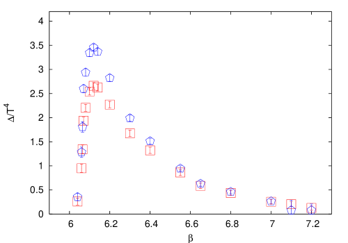
Figure 1: $\Delta/T^{4}$ as a function of the bare coupling $\beta$ using a non-perturbative (squares) and one-loop order perturbative (pentagons) $\beta$-function, $B(\alpha_{s})$. The results agree for $\beta\geq 6.5$. The data of boyd for $N_{\tau}=8$ has been used in this analysis.

Direct application of the derivatives in eq. (11) to the expression for $\epsilon$ in eq. (12) would give an incorrect result for $C_{\scriptscriptstyle V}$, i.e., $C_{\scriptscriptstyle V}/T^{3}$ would not give the correct ideal gas value ($4\epsilon/T^{4}$) in the limit $g\rightarrow 0$. This is because we have chosen to work with the variables $\xi$ and $a_{s}$, whereby the dimensions of both $T$ and $V$ come from powers of $a_{s}$. Application of the derivative formulæ therefore see false scalings of these quantities. We solve this problem by choosing to work in terms of a dimensionless ratio so that the scaling is automatically taken care of. We define

$${\cal C}=\frac{\Delta}{\epsilon}\qquad{\rm and}\qquad\Gamma=T\left.\frac{\partial{\cal C}}{\partial T}\right|_{V},$$ (14)

where ${\cal C}$ is the conformal measure already discussed. Then, using eqs. (6, 14) one can proceed straightaway to write

$$\frac{C_{\scriptscriptstyle V}}{T^{3}}=\left(\frac{\epsilon/T^{4}}{P/T^{4}}\right)\left[\frac{s}{T^{3}}+\frac{\Gamma}{3}\frac{\epsilon}{T^{4}}\right],\qquad{\rm and}\qquad C_{s}^{2}=\left(\frac{P/T^{4}}{\epsilon/T^{4}}\right)\left[1+\frac{\Gamma\epsilon/T^{4}}{3s/T^{3}}\right]^{-1}.$$ (15)

In order to complete these expression, one needs to express $\Gamma$ in terms of quantities computable on the lattice.

We lighten the subsequent formulæ by defining the two functions

$$F(\xi,a_{s})=\frac{\Delta a_{s}^{4}}{6N_{c}\xi}=a_{s}\left[\frac{\partial K_{s}}{\partial a_{s}}D_{s}+\frac{\partial K_{\tau}}{\partial a_{s}}D_{t}\right],\qquad{\rm and}\qquad G(\xi,a_{s})=\frac{-\epsilon a_{s}^{4}}{6N_{c}\xi}=\xi\left[\frac{\partial K_{s}}{\partial\xi}D_{s}+\frac{\partial K_{\tau}}{\partial\xi}D_{t}\right].$$ (16)

Since ${\cal C}=-F/G$, one finds that

$$\Gamma=-\frac{T}{G}\left.\frac{\partial F}{\partial T}\right|_{V}+\frac{TF}{G^{2}}\left.\frac{\partial G}{\partial T}\right|_{V}.$$ (17)

The derivatives of $F$ and $G$ involve the variances and covariances of the spatial and temporal plaquettes. The complete expressions are given in Appendix A. We also need to write down the second derivatives of the couplings—

$$a_{s}\frac{\partial K_{s}^{\prime}}{\partial a_{s}}=-\frac{B(\alpha_{s})}{2\pi\alpha_{s}^{2}\xi^{2}},\quad K_{s}^{\prime\prime}=\frac{2g_{s}^{-2}}{\xi^{3}}-\frac{2c_{s}^{\prime}}{\xi^{2}}+\frac{c_{s}^{\prime\prime}}{\xi},\qquad a_{s}\frac{\partial K_{\tau}^{\prime}}{\partial a_{s}}=\frac{B(\alpha_{s})}{2\pi\alpha_{s}^{2}},\quad K_{\tau}^{\prime\prime}=2c_{\tau}^{\prime}+\xi c_{\tau}^{\prime\prime}.$$ (18)

Details of the evaluation of the second order Karsch coefficients $c_{s,\tau}^{\prime\prime}$ are given in Appendix B. For $N_{c}=3$ their numerical values are $c_{s}^{\prime\prime}=-0.298193$ and $c_{\tau}^{\prime\prime}=0.333670$.

It is known Heller that in the weak-coupling limit, i.e., for $g\to 0$, the dominant contribution to all plaquettes varies as $g^{2}$. So the $D_{i}$’s also vary as $g^{2}$. Hence in this limit $\Delta/T^{4}\propto g^{2}$ and can be neglected in comparison with $\epsilon/T^{4}$ which is $(N_{c}^{2}-1)\pi^{2}/15+{\cal O}(g^{2})$. As shown in Appendix A, $\Gamma\to 0$ in this limit. As a result, $C_{\scriptscriptstyle V}/T^{3}\to 4\epsilon/T^{4}$ and $C_{s}^{2}\to 1/3$. Note that in any conformal invariant theory in $d+1$ dimensions one has $\epsilon=dP$, i.e., ${\cal C}=\Gamma=0$, and hence, by eq. (15), $C_{s}^{2}=1/d$ and $C_{\scriptscriptstyle V}/T^{3}=(d+1)\epsilon/T^{4}$.

II.3 On the method

The formalism outlined in Section II.1 corresponds to the so-called “differential” method. On the other hand, about a decade back a new method called the “integral” method was employed boyd to find the equation of state of QCD matter. This consists of using the expression for $\Delta/T^{4}$ in eq. (13) while eschewing the expression for $\epsilon/T^{4}$ in favour of a totally different method for determining $P/T^{4}$. This proceeds from the observation that $P=(T/V)\ln{\cal Z}$ for a homogeneous system. Since lattice computations do not determine the absolute normalization of ${\cal Z}$, use of this formula requires fixing an additive constant. In boyd this constant was fixed by setting $P=0$ in the low temperature phase of QCD, slightly below $T_{c}$.

This leads to a conceptual problem. Since the pure gauge phase transition in QCD is of first order, the system is not homogeneous at $T_{c}$ and the method is not strictly applicable there. One makes an unknown systematic error in integrating through $T_{c}$. This is in addition to a small systematic error due to setting $P=0$ just below $T_{c}$ and the numerical integration errors. However, a decade ago, these errors were deemed to be smaller than the scale errors in the “differential” method which could give rise even to negative pressure in computations with coarse lattice spacings, $a=1/TN_{\tau}$, which were the only ones possible then.

The two methods must agree in the continuum limit. A reanalysis of the data of boyd showed that the two methods agreed to within 5% (i.e., within statistical errors) for $T\geq 2T_{c}$ sgupta already for $N_{\tau}=8$, i.e., for $a=1/16T_{c}$. In fact a criterion for the agreement is straightforward, and follows from the fact the expression for $\Delta/T^{4}$ is common to the two methods. Since the integral method does not need the Karsch coefficients, it allows one to use a non-perturbatively determined $\beta$-function $B(\alpha_{s})$. On the other hand, the differential method requires, for internal consistency, that the Karsch coefficients and $B(\alpha_{s})$ be obtained at the same order, i.e., at one-loop order in the present state of the art.

Thus, a comparison between the values of $\Delta/T^{4}$ extracted for a given $N_{\tau}$ using the two techniques would reveal at what $T$ the two methods become identical. Then, using asymptotic scaling, one could also give the minimum value of $N_{\tau}$ which would be required for the same level of agreement as a function of $T$. Such a comparison is shown in Figure 1 and demonstrates that a bare coupling of $\beta\geq 6.55$ already suffices.

The use of the “differential” method does require small lattice spacings, but this is currently quite feasible with modern computers. The advantage is that the formalism of Section II.2 can be used to compute second derivatives of the free energy as operator expectation values. If the EOS were to be evaluated by the “integral” method, then these quantities could only be evaluated by numerical differentiation iitk , which is a less attractive solution.

$T/T_{c}$	$\beta$	Asymmetric Lattice		Symmetric Lattice
		size	stat.	size	stat.
2.0	6.0625	$4\times 8^{3}$	60000	$22^{4}$	38000
		$~{}\times 10^{3}$	56000
		$~{}\times 12^{3}$	50000
		$~{}\times 14^{3}$	51000
		$~{}\times 16^{3}$	51000
	6.5500	$8\times 18^{3}$	1100000	$12^{4}$	800000
				$16^{4}$	626000
				$18^{4}$	802000
				$22^{4}$	552000
				$32^{4}$	330000
	6.7500	$10\times 22^{3}$	1100000	$22^{4}$	969000
	6.9000	$12\times 26^{3}$	1040000	$26^{4}$	550000
	7.0000	$14\times 30^{3}$	425000	$30^{4}$	146000
3.0	6.3384	$4\times 10^{3}$	220000	$22^{4}$	75000
		$~{}\times 12^{3}$	200000
		$~{}\times 16^{3}$	200500
		$~{}\times 20^{3}$	210000
		$~{}\times 22^{3}$	150000
	7.0500	$10\times 32^{3}$	560000	$32^{4}$	146000
	7.2000	$12\times 38^{3}$	315000	$38^{4}$	58000

Table 1: The coupling ($\beta$), lattice sizes ($N_{\tau}\times N_{s}^{3}$), statistics and symmetric lattice sizes ($N_{s}^{4}$) are given for each temperature. Statistics means number of sweeps used for measurement of plaquettes after discarding for thermalization.

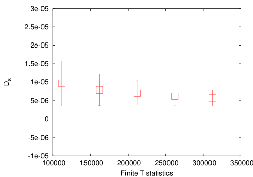
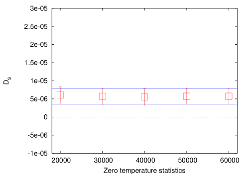
Figure 2: Stability of $D_{s}$ against the statistics in $T>0$ (first panel) and $T=0$ (second panel) simulations. The coupling corresponds to $3T_{c}$ on a $12\times 38^{3}$ lattice and the corresponding $T=0$ simulation was performed on a $38^{4}$ lattice. In both the figures we have also plotted the 1-$\sigma$ error band of the final errors.

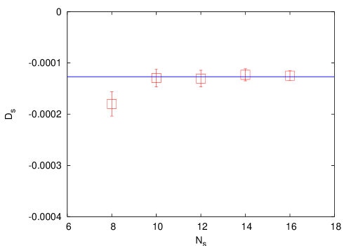
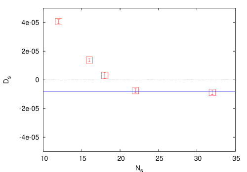
Figure 3: Dependence of $D_{s}$ against the spatial size, $N_{s}$, of the $T>0$ lattice for $2T_{c}$ and $22^{4}$ lattice for the $T=0$ computation (left panel). We have shown a fit to a constant through the three largest lattices. Dependence of $D_{s}$ on $N_{s}$ for the $T=0$ lattice when the $2T_{c}$ computation is performed on an $8\times 18^{3}$ lattice (right panel). A fit to a constant with the two largest sizes is also shown.

$N_{\tau}$	$36N_{c}^{2}N_{\tau}^{4}V\sigma_{s,s}$	$36N_{c}^{2}N_{\tau}^{4}V\sigma_{\tau,\tau}$	$36N_{c}^{2}N_{\tau}^{4}V\sigma_{s,\tau}$
10	$(0.2\pm 1.0)\times 10^{-5}$	$(0.2\pm 1.0)\times 10^{-5}$	$(0.1\pm 1.0)\times 10^{-5}$
12	$(0.7\pm 4.1)\times 10^{-4}$	$(0.7\pm 4.1)\times 10^{-4}$	$(0.4\pm 3.5)\times 10^{-4}$
14	$(0.1\pm 1.4)\times 10^{-3}$	$(0.1\pm 1.5)\times 10^{-3}$	$(0.1\pm 1.3)\times 10^{-3}$

Table 2: Contributions of different covariances, with their respective errors, are tabulated for different $N_{\tau}$ at $2T_{c}$. This shows all the contributions are totally negligible.

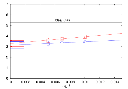
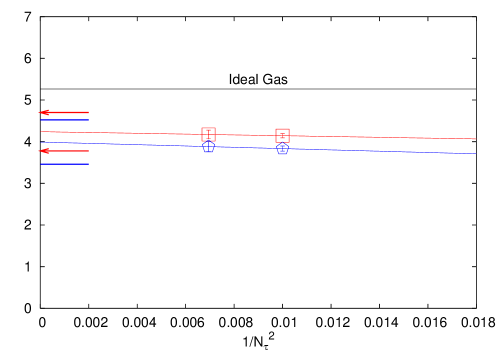
Figure 4: Dependence of $\epsilon/T^{4}$ (squares) and $3P/T^{4}$ (pentagons) on $1/N_{\tau}^{2}$ for $T=2T_{c}$ (left panel) and $T=3T_{c}$ (right panel). The 1-$\sigma$ error band of the continuum values has been indicated by arrows (for $\epsilon/T^{4}$) and lines (for $3P/T^{4}$).

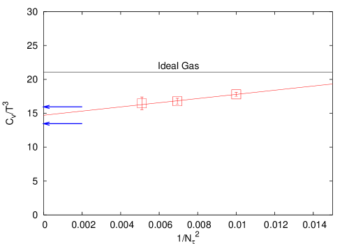
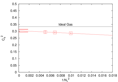
Figure 5: Dependence of $C_{\scriptscriptstyle V}/T^{3}$ (left panel) and $C_{s}^{2}$ (right panel) on $1/N_{\tau}^{2}$ at $T=2T_{c}$. The 1-$\sigma$ error band of the continuum values has been indicated by the arrows.

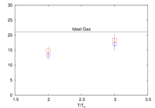
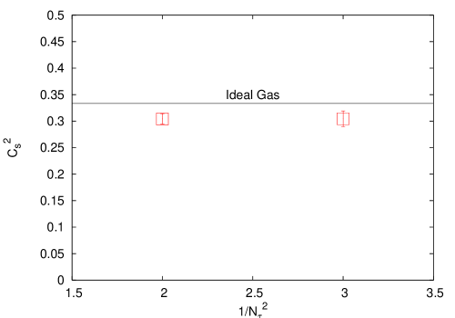
Figure 6: In the left panel we show the continuum values of $4\epsilon/T^{4}$ (pentagons) and $C_{\scriptscriptstyle V}/T^{3}$ (squares) against $T/T_{c}$. In the right panel we show the temperature dependence of the continuum extrapolated values of $C_{s}^{2}$.

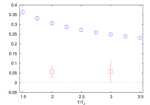
Figure 7: Continuum values of the conformal measure, ${\cal C}$, (squares) and the one-loop order $\beta$-function (circles) evaluated at the scale $2\pi T$. For the $T=0$ gluon condensate see the text.

III Simulations and results

The simulations have been performed using the Cabbibo-Marinari pseudo-heatbath algorithm with Kennedy-Pendleton updating of three $SU(2)$ subgroups on each sweep. Plaquettes were measured on each sweep. For each simulation we discarded around 5000 initial sweeps for thermalization. We found that integrated autocorrelation time for the plaquettes never exceeded $3$ sweeps. In Table 1 we give the details of our runs. All errors were calculated by the jack-knife method, where the length of each deleted block was chosen to be at least six times the maximum integrated autocorrelation time of all the simulations used for that calculation.

Of all the quantities which go into determining the equation of state, namely $D_{s}$, $D_{t}$ and $D_{s}-D_{t}$, we found that $D_{s}$ was the smallest. Hence control over the errors of $D_{s}$ was the most stringent requirement on the amount of statistics needed. In Figure 2 we show the stability of $D_{s}$ against the finite temperature and zero temperature statistics for the case where we have minimum statistics, namely for the $3T_{c}$ run on the $12\times 38^{3}$ lattice and the run at the same coupling on the $38^{4}$ lattice. Note that the plaquette values are of the order of unity, and the first four digits cancel in computing $D_{s}$. Thus, the control over errors shown in Figure 2 was due to our reducing the errors in the plaquette variables to a few parts per million.

We checked the stability of $D_{s}$ against the spatial size of the $T>0$ lattice. The left panel of Figure 3 displays the dependence of $D_{s}$ on $N_{s}$ for $N_{\tau}=4$ when the temperature is $2T_{c}$ and the symmetric lattice size is $22^{4}$. We have also shown a fit to a constant using the data on the three largest lattices. These fits pass through the data collected on the $N_{s}=(T/T_{c})N_{\tau}+2$ lattice. We have checked that this condition holds for $3T_{c}$ also. This observation is consistent with the results of earlier investigation of finite size effects for $T>0$ saumen and motivated our choice of $N_{s}=(T/T_{c})N_{\tau}+2$.

We also investigated the dependence of $D_{s}$ on the size of the symmetric $N_{s}^{4}$ lattice used for the $T=0$ subtraction. The right panel of Figure 3 exhibits the dependence of $D_{s}$ on $N_{s}$ for a run at $2T_{c}$ on a $8\times 18^{3}$ lattice. $D_{s}$ is seen to be constant for $N_{s}\geq 22$. In view of this we have used $22^{4}$ as our minimum $T=0$ lattice size, and scaled this up with changes in the lattice spacing.

We evaluated the contributions of the terms containing different covariances of the plaquettes and found them to be totally negligible, as shown in Table 2. It is worth noting that a previous computation in $SU(2)$ pure gauge theory close to $T_{c}$ found significantly larger, and clearly non-vanishing, variances of the plaquettes gavai . This suggests that the variance terms might make significant contributions to the specific heat and speed of sound closer to the softest point of the EOS.

Following the observation illustrated in Figure 1, all our continuum extrapolations have been done with lattice spacings which are at least as small as that at $\beta=6.55$. For $T=2T_{c}$ this leaves three values of $N_{\tau}$ from which an continuum extrapolation linear in $a^{2}\propto 1/N_{\tau}^{2}$ can be performed. However, at $T=3T_{c}$, the continuum extrapolation has been performed with two values of $N_{\tau}$. This completely fixes the two parameters of the linear extrapolation to the continuum and the error in the continuum extrapolated value is by definition zero. In this case the error in the continuum value was estimated by three methods. Two of these consisted of first making the best fit using two parameters, and then keeping one fixed while allowing the other to vary in order to make an estimate of the error in that parameter. We also made extrapolations using the upper end of one error bar and the lower end of the other. This last procedure gave the maximum errors in the continuum extrapolated values, and we choose to quote this, since it is the most conservative error estimate.

In Figure 4 we present our results for $\epsilon$ and $P$. At $3T_{c}$ the continuum limit values of $\epsilon/T^{4}$ and $P/T^{4}$ differ from their respective ideal gas values ($8\pi^{2}/15$ and $8\pi^{2}/45$ respectively) by about 24%, and by about 40% at $2T_{c}$. This is consistent with previous measurements of the equation of state at these temperatures. At $2T_{c}$ our results differ from the ideal gas value by almost 7-$\sigma$. The actual results are also collected in Table 3.

Similar continuum extrapolation of $C_{\scriptscriptstyle V}/T^{3}$ and $C_{s}^{2}$ are shown in Figures 5 and Figures 6 respectively. Continuum extrapolated values of different quantities for two temperatures are tabulated in Table 3. It can be seen that although $\epsilon/T^{4}$ and $P/T^{4}$ differ significantly from their ideal gas values, $C_{s}^{2}$ is quite close to $1/3$, being within 2-3 $\sigma$. Similarly, it can be seen that $C_{\scriptscriptstyle V}/T^{3}$ is completely compatible with $4\epsilon/T^{4}$, a fact also illustrated in Figure 7. However, its deviation from the ideal gas value is seen to be more significant.

The generation of a scale and the consequent breaking of conformal invariance at short distances in QCD is quantified by the $\beta$-function of QCD, and at long distance in the finite temperature plasma by the conformal measure ${\cal C}$. In Figure 7 we plot these two together. The $T=0$ gluon condensate, $\langle F^{2}\rangle_{0}$ gives a measure of the non-perturbative strength of the breaking of conformal invariance at $T=0$. A recent estimate badalian gives $\langle F^{2}\rangle_{0}/\Lambda_{\overline{\scriptscriptstyle MS}}^{4}=10.5\pm 0.5$, where $\Lambda_{\overline{\scriptscriptstyle MS}}$ is compatible with the value used to set the temperature scale. It is clear that conformal invariance is better respected in the finite temperature effective long-distance theory than at the microscopic scale.

An alternative measure of conformal symmetry breaking for $T>0$ could be the dimensionless quantity

$${\cal C}^{\prime}\equiv\frac{\Delta}{\langle F^{2}\rangle_{0}}={\cal C}\frac{\epsilon}{\langle F^{2}\rangle_{0}}={\cal C}\left(\frac{\epsilon}{T^{4}}\right)\left(\frac{T}{\Lambda_{\overline{\scriptscriptstyle MS}}}\right)^{4}\left(\frac{\langle F^{2}\rangle_{0}}{\Lambda_{\overline{\scriptscriptstyle MS}}^{4}}\right)^{-1}.$$ (19)

Clearly its use is limited to making the trivial point that the scale $T$ breaks conformal symmetry explicitly, reflected by the $T^{4}$ growth of ${\cal C}^{\prime}$. This misses physics on both the weak-coupling and the strong coupling AdS/CFT sides. On one side is the likelihood that the weak coupling expansion, which is conformal, becomes more accurate at sufficiently high temperature— although $\Delta$ increases with $T$, $\Delta/T^{4}$ becomes a small part of $\epsilon/T^{4}$, $P/T^{4}$ or $s/T^{4}$. On the other hand is the possibility that AdS/CFT is accurate because the $T$ dependence can be taken into the dimension of operators, and the CFT shows up in non-trivial dimensionless quantities such as the function $f$ in eq. (2). ${\cal C}$ allows us to test the accuracy of these possibilities, thereby capturing the interesting facts shown in Figure 6, whereas ${\cal C}^{\prime}$ misses them.

$T/T_{c}$	$g^{2}N_{c}$	$\epsilon/T^{4}$	$P/T^{4}$	$s/T^{3}$	$C_{\scriptscriptstyle V}/T^{3}$	$C_{s}^{2}$
2.0	8.1 (1)	3.3 (3)	1.0 (1)	4.2 (3)	15 (1)	0.30 (1)
3.0	7.0 (1)	4.2 (5)	1.3 (2)	5.6 (6)	18 (2)	0.30 (2)

Table 3: Continuum values of some quantities at the two temperatures we have explored. The numbers in brackets are the error on the least significant digit. The value of the t’Hooft coupling $N_{c}g^{2}$ is computed at the scale $2\pi T$ using the $T_{c}/\Lambda_{\overline{\scriptscriptstyle MS}}$ quoted in sgupta .

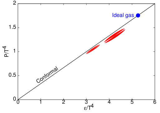
Figure 8: The equation of state of QCD matter. The diagonal line denotes possible EOS for theories with conformal symmetry. The circle on the diagonal denotes the ideal gluon gas, whose EOS in this form is temperature independent. The ellipses denote 66% error bounds on the measured EOS. The ratio of the axes is a measure of the covariance in the measurements of $\epsilon/T^{4}$ and $P/T^{4}$, which is about 90%. The wedges piercing these ellipses have average slope $C_{s}^{2}$, and the opening half-angle of these wedges indicate the error in $C_{s}^{2}$.

IV Discussion

In this paper we have determined the continuum limits of the specific heat at constant volume, $C_{\scriptscriptstyle V}$, and the speed of sound, $C_{s}$, in the continuum limit of the pure gluon plasma. In the process we have also recomputed the EOS, i.e., the pressure, $P$, and the energy density, $\epsilon$, by a method which has not been used earlier to obtain the continuum limit. Our results are collected together in Table 3. It is clear from this that the plasma phase is not far from the conformal symmetric limit, in which $C_{s}^{2}=1/3$ and $C_{\scriptscriptstyle V}/T^{3}=4\epsilon/T^{4}$. This is also illustrated in Figures 6 and 7. The latter figure further shows that conformal symmetry is more nearly realized on length scale of order $T$ than one would expect either from the $\beta$-function of QCD or from the gluon condensate $\langle F^{2}\rangle_{0}$.

We have extended the operator method for the EOS in order to obtain these results. We have limited our computations to lattice spacings where the method is guaranteed to work because of the observed scaling of results with the correct QCD beta function, as shown in Figure 1. The main advantage of this method is the relatively noise-free determination of $C_{s}$ and $C_{\scriptscriptstyle V}$.

There is as yet no unambiguous determination of these quantities from experiments. Hydrodynamic analyses of RHIC data routinely use $C_{s}^{2}=1/3$ in the plasma phase; our results show that this receives a correction of up to 10% in QCD. It would be interesting to check the sensitivity of the RHIC data to the variation in $C_{s}^{2}$ and compare the bounds there with our lattice results. Little is known yet about $C_{\scriptscriptstyle V}$. The only estimate that we are aware of korus uses the data on $p_{\scriptscriptstyle T}$ fluctuations from appelshauser to obtain $C_{\scriptscriptstyle V}/T^{3}=60\pm 100$ for $T=180$ MeV.

Our data on the entropy density, $s/T^{3}$, shown in Table 3 can be used to test the quantitative predictions of the strong-coupling expansion of the ${\cal N}=4$ supersymmetric Yang-Mills theory in gubser . Eq, (2) should interpolate the ratio $s/s_{0}$ between the strong-coupling limit of 3/4 and the weak-coupling limit of 1. It is clear that at $T=2T_{c}$ this ratio is below 3/4, and hence cannot be described by the computation in gubser . At $3T_{c}$, the ratio is above 3/4 and there is quantitative agreement with the formula of gubser using the value of the t’Hooft coupling quoted in Table 3. It is interesting that this particular strong-coupling theory fails at temperatures where weak coupling theories also break down.

A partial summary of our results is illustrated by plotting the equation of state as $P/T^{4}$ against $\epsilon/T^{4}$, as in Figure 8. In this plot, the ideal gas for fixed number of colours is represented by a single point which is independent of $T$, and theories with conformal symmetry by the line $\epsilon=3P$. Pure gauge QCD lies close to the conformal line at high temperature, as shown. One expects the EOS to drop well below this line near $T_{c}$, since the theory then contains massive hadrons (glueballs in pure gluon QCD) with masses in excess of $T_{c}$. Thus one expects the origin to be approached almost horizontally as $T\to 0$. We will present data closer to, and below, $T_{c}$ in a forthcoming paper.

SG would like to thank Jean-Paul Blaizot, Kari Eskola, Rajesh Gopakumar, Pasi Huovinen, Toni Rebhan and Vesa Ruuskanen for discussions. RVG would like to thank the Alexander von Humboldt Foundation for financial support and the members of the Theoretical Physics Department of Bielefeld university for their kind hospitality. SM would like to thank Rajarshi Ray for discussions and for his help in calculating the derivatives of Karsch Coefficients. SM would also like to thank TIFR Alumni Association for partial financial support.

Appendix A Derivatives of F and G

From the definition of $F$ in eq. (16) we obtain

$$\left.\frac{\partial F}{\partial\xi}\right|_{a_{s}}=a_{s}\left[\frac{\partial K_{s}^{\prime}}{\partial a_{s}}D_{s}+\frac{\partial K_{\tau}^{\prime}}{\partial a_{s}}D_{t}\right]+a_{s}\left[\frac{\partial K_{s}}{\partial a_{s}}D_{s}^{\prime}+\frac{\partial K_{\tau}}{\partial a_{s}}D_{t}^{\prime}\right].$$ (20)

Since the plaquette operators do not explicitly depend on $\xi$ (or $a_{s}$), we can easily take the derivative—

$$D_{i}^{\prime}=D_{i}\langle S^{\prime}\rangle-\langle(P_{i}-P_{0})S^{\prime}\rangle=-6N_{c}N_{\tau}N_{s}^{3}\left[K_{s}^{\prime}\sigma_{s,i}+K_{\tau}^{\prime}\sigma_{\tau,i}\right],$$ (21)

where $\sigma_{s,i}=\langle D_{s}D_{i}\rangle-\langle D_{s}\rangle\langle D_{i}\rangle$ and $\sigma_{\tau,i}=\langle D_{t}D_{i}\rangle-\langle D_{t}\rangle\langle D_{i}\rangle$ are the variances and covariances of the plaquettes. Next, using Eq (10) and Eq (18), the $\xi\rightarrow 1$ limit becomes

$$\left.\frac{\partial F}{\partial\xi}\right|_{a_{s}}=\frac{B(\alpha_{s})}{2\pi\alpha_{s}^{2}}\left[D_{t}-D_{s}\right]-6N_{c}N_{\tau}N_{s}^{3}\frac{B(\alpha_{s})}{2\pi\alpha_{s}^{2}}\left[\frac{\sigma_{\tau,\tau}-\sigma_{s,s}}{g^{2}}+c_{s}^{\prime}\sigma_{s,s}+c_{\tau}^{\prime}\sigma_{\tau,\tau}+(c_{s}^{\prime}+c_{\tau}^{\prime})\sigma_{s,\tau}\right].$$ (22)

Similarly we find

$$\left.\frac{\partial G}{\partial\xi}\right|_{a_{s}} = \frac{D_{s}+D_{t}}{g^{2}}-c_{s}^{\prime}D_{s}+3c_{\tau}^{\prime}D_{t}+c_{s}^{\prime\prime}D_{s}+c_{\tau}^{\prime\prime}D_{t}-6N_{c}N_{\tau}N_{s}^{3}\times$$ (23)

$$\qquad\left[\frac{\sigma_{s,s}+\sigma_{\tau,\tau}-2\sigma_{s,\tau}}{g^{4}}+\frac{2(c_{\tau}^{\prime}\sigma_{\tau,\tau}+c_{s}^{\prime}\sigma_{s,\tau}-c_{s}^{\prime}\sigma_{s,s}-c_{\tau}^{\prime}\sigma_{s,\tau})}{g^{2}}+{c_{s}^{\prime}}^{2}\sigma_{s,s}+{c_{\tau}^{\prime}}^{2}\sigma_{\tau,\tau}+2c_{s}^{\prime}c_{\tau}^{\prime}\sigma_{s,\tau}\right].$$

Since $D_{i}\sim g^{2}$ and $\sigma_{i,j}\sim g^{4}$ in the limit $g\to 0$, $\partial F/\partial\xi\to 0$ but $\partial G/\partial\xi$ remains finite. As a result, $\Gamma\to 0$, in this limit, as it should, even when the variances of the plaquettes are taken into account.

Appendix B Second order Karsch coefficients

Expressions for $c_{s}(\xi)$ and $c_{\tau}(\xi)$ as given in Kar are

$$c_{s}(\xi) = 4N_{c}\left[\frac{N_{c}^{2}-1}{24N_{c}^{2}}\left(I_{1}(\xi)-\frac{3}{4}\right)-\frac{5}{288}I_{2a}(\xi)+\frac{1}{48}I_{3}(\xi)+\frac{1}{128}I_{4}(\xi)+\frac{11}{12}FIN(\xi)+0.010245\right],$$

$$c_{\tau}(\xi) = 4N_{c}\left[\frac{N_{c}^{2}-1}{24N_{c}^{2}}\left(\frac{1}{3\xi^{2}}I_{1}(\xi)+\frac{1}{\xi}I_{5}(\xi)-\frac{1}{2}\right)+\frac{1}{64}I_{3}(\xi)-\frac{5}{576}I_{2a}(\xi)\right]$$ (24)

$$\qquad+4N_{c}\left[\frac{1}{256\xi^{2}}I_{4}(\xi)-\frac{1}{48\xi^{2}}I_{6}(\xi)-\frac{1}{192\xi^{2}}I_{7}(\xi)+\frac{11}{12}FIN(\xi)+0.010245\right].$$

Here $b^{2}=\sin^{2}x_{1}+\sin^{2}x_{2}+\sin^{2}x_{3}$, and

$$I_{1}(\xi) = \xi\left(\frac{2}{\pi}\right)^{3}\int d^{3}xb(\xi^{2}+b^{2})^{-1/2},$$

$$I_{2a}(\xi) = \xi\left(\frac{2}{\pi}\right)^{3}\int d^{3}xb^{-1}(\xi^{2}+2b^{2})(\xi^{2}+b^{2})^{-3/2},$$

$$I_{2b}(\xi) = \xi^{3}\left(\frac{2}{\pi}\right)^{3}\int d^{3}x\left[b(\xi^{2}+b^{2})^{1/2}\left(b+(\xi^{2}+b^{2})^{1/2}\right)^{2}\right]^{-1},$$

$$I_{3}(\xi) = \xi\left(\frac{2}{\pi}\right)^{3}\int d^{3}x\sin^{2}x_{1}\sin^{2}x_{2}\frac{\xi^{2}+2b^{2}}{b^{3}(\xi^{2}+b^{2})^{3/2}},$$

$$I_{4}(\xi) = \xi\left(\frac{2}{\pi}\right)^{3}\int d^{3}x\sin^{2}2x_{1}\frac{\xi^{2}+2b^{2}}{b^{3}(\xi^{2}+b^{2})^{3/2}},$$

$$I_{5}(\xi) = \xi^{2}\left(\frac{2}{\pi}\right)^{3}\int d^{3}x(\xi^{2}+b^{2})^{-1/2}\left[b+(\xi^{2}+b^{2})^{1/2}\right]^{-1},$$

$$I_{6}(\xi) = \xi^{3}\left(\frac{2}{\pi}\right)^{3}\int d^{3}xb^{-1}(\xi^{2}+b^{2})^{-3/2}\cos^{2}x_{1},$$

$$I_{7}(\xi) = \xi^{3}\left(\frac{2}{\pi}\right)^{3}\int d^{3}xb^{-1}(\xi^{2}+b^{2})^{-3/2},$$ (25)

Limits of all the above integrals are $[0,\pi/2]$. And :

$$DIV(\xi) = \frac{1}{(2\pi)^{4}}\int\int_{-\pi/2}^{\pi/2}\int d^{3}x\int_{-\pi\xi/2}^{\pi\xi/2}dx_{4}\left[b^{2}+\xi^{2}\sin^{2}(x_{4}/\xi)\right]^{-2},$$

$$FIN(\xi) = DIV(\xi)-DIV(1).$$ (27)

The integral $DIV(\xi)$ is infrared divergent. However, what actually needed here is $FIN(\xi)$. $FIN(\xi)$ is not divergent as it is constructed by subtracting the integral $DIV(1)$, having the same infrared divergence as that of $DIV(\xi)$, from $DIV(\xi)$. The derivatives of $FIN(\xi)$ are just the derivatives of $DIV(\xi)$ which are not divergent. We calculated $FIN^{\prime\prime}(1)$ by direct numerical integration and also by taking a derivative of $FIN^{\prime}(\xi)$, at $\xi=1$, numerically. We found that values obtained from both the methods are consistent.

	$I_{1}$	$I_{2a}$	$I_{2b}$	$I_{3}$	$I_{4}$	$I_{5}$	$I_{6}$	$I_{7}$	$FIN$
Integrals	0.750000	0.929600	0.119734	0.103289	0.478934	0.250000	0.206578	0.309867	0.0
$1$-st derivatives	0.440133	0.208546	0.190133	0.033774	0.065779	0.309867	0.238384	0.411188	0.003166
$2$-nd derivatives	-0.518412	-0.663270	0.030921	-0.088777	-0.262319	-0.101321	-0.146561	-0.159106	-0.014471

Table 4: Values of the integrals $I_{x}(\xi)$ ’s and $FIN(\xi)$ and their derivatives with respect to $\xi$ at $\xi=1$.

The numerical values of all these above integrals and their derivatives with respected to $\xi$, at $\xi=1$, are tabulated in Table 4. Using these values we can obtain $\xi$ derivatives of the Karsch coefficients at $\xi=1$

$$c_{s}^{\prime}=4N_{c}\left[\frac{N_{c}^{2}-1}{32N_{c}^{2}}0.586844+0.000499\right],$$

$$c_{s}^{\prime\prime}=4N_{c}\left[\frac{1-N_{c}^{2}}{32N_{c}^{2}}0.691216-0.005649\right],$$

$$c_{\tau}^{\prime}=4N_{c}\left[\frac{1-N_{c}^{2}}{32N_{c}^{2}}0.586844+0.005306\right],$$

$$c_{\tau}^{\prime\prime}=4N_{c}\left[\frac{N_{c}^{2}-1}{32N_{c}^{2}}1.038595-0.001044\right].$$ (28)

The values of all the integrals and their first derivatives as well as the regular Karsch coefficients match with their respective values mentioned in Kar .

References

-
(1)
G. Boyd et al, Phys. Rev. Lett., 75 (1995) 4169;
G. Boyd et al, Nucl. Phys., B 469 (1996) 419. -
(2)
P. Arnold and C. Zhai, Phys. Rev., D 50 (1994) 7603, ibid., D 51 (1995) 1906;
E. Braaten and A. Nieto, Phys. Rev., D 53 (1996) 3421;
K. Kajantie et al., Phys. Rev. Lett., 86 (2001) 10, J. H. E. P., 0304 (2003) 036. - (3) S. S. Gubser, I. R. Klebanov and A. A. Tseytlin, Nucl. Phys., B 534 (1998) 202.
- (4) G. Policastro, D. T. Son and A. Starinets, Phys. Rev. Lett.87 (2001) 081601.
- (5) D. Teaney, Phys. Rev., C 68 (2003) 034913.
- (6) A. Nakamura and S. Sakai, hep-lat/0406009.
- (7) S. Gupta, Phys. Lett., B 597 (2004) 57.
- (8) A. Peshier, Nucl. Phys.A 702 (2002) 128.
- (9) E. Shuryak, Prog. Nucl. Part. Phys., 53 (2004) 273.
-
(10)
J. O. Anderson et al., Phys. Rev., D 66 (2002) 085016;
J.-P. Blaizot, E. Iancu and A. Rebhan, Phys. Rev., D 63 (2001) 065003. - (11) A. Dumitru, J. Lenaghan and R. D. Pisarski, hep-ph/0410294.
- (12) J. Ollitrault, Phys. Rev., D 46 (1992) 229.
- (13) H. Sorge, Phys. Rev. Lett., 82 (1999) 2048.
-
(14)
P. F. Kolb et al., Phys. Lett., B 459 (1999) 667;
P. F. Kolb et al., Nucl. Phys., A 661 (1999) 346. -
(15)
D. Teaney et al., Phys. Rev. Lett., 86 (2001) 4783;
D. Teaney et al., nucl-th/0110037. - (16) B. Mohanty et al., Phys. Rev.C 67 (2003) 024904.
- (17) M. Gaździcki et al., Phys. Lett., B 585 (2004) 115.
- (18) L. Stodolsky, Phys. Rev. Lett.75 (1995) 1044.
- (19) R. Korus et al., Phys. Rev., C 64 (2001) 054908.
- (20) J. Engels et al, Nucl. Phys., B 205 [FS5] (1982) 545.
- (21) Y. Deng, Nucl. Phys., B (Proc. Suppl.) 9 (1989) 334.
- (22) S. Gupta, Phys. Rev., D 64 (2001) 034507.
- (23) S. Gupta, Pramana, 61 (2003) 877.
- (24) A. Hasenfratz et al, Nucl. Phys., B 193 (1981) 210.
- (25) J. Engels et al, Nucl. Phys., B 205 [FS5] (1982) 239.
- (26) F. Karsch, Nucl. Phys.B 205 [FS5] (1982) 285.
- (27) G. P. Lepage et al, Phys. Rev., D 48 (1993) 2250.
- (28) R. G. Edwards et al, Nucl. Phys., B 517 (1998) 377.
- (29) U. Heller et al, Nucl. Phys., B 251 [FS13] (1985) 254.
- (30) S. Datta and S. Gupta, Phys. Lett., B471 (2000) 382.
- (31) S. Datta and R. V. Gavai, Phys. Rev.D 60 (1999) 034505.
- (32) H. Appelshäuser et al, Phys. Lett., B 459 (1999) 679.
- (33) A. M. Badalian and B. L. G. Bakker, hep-ph/0412030.