The monopole content of topological clusters :
have KvB calorons been found?

Abstract

Using smearing of equilibrium lattice fields generated at finite temperature in the confined phase of $SU(2)$ lattice gauge theory, we have investigated the emerging topological objects (clusters of topological charge). Analysing their monopole content according to the Polyakov gauge and the maximally Abelian gauge, we characterize part of them to correspond to nonstatic calorons or static dyons in the context of Kraan-van Baal caloron solutions with non-trivial holonomy. The behaviour of the Polyakov loop inside these clusters and the (model-dependent) topological charges of these objects support this interpretation.

I Introduction

The space-time distribution of topological charge in the Euclidean vacuum, as it can be made visible in lattice gauge theory (LGT), has continued to be an interesting topic, being the source of chiral symmetry breaking and a manifestation of the $U_{A}(1)$ anomaly. In this context, the relation to the confining property of the vacuum has been mostly left out of consideration. The guiding line of this activity was the instanton liquid model ILM , originally motivated by the semiclassical approximation, which then has turned into a successful and sufficiently rich model of the gluonic background of hadron physics.  The inability of the instanton model to describe confinement was not considered as an essential disadvantage. The semiclassical background of the model itself has suggested to employ (limited) cooling as the method of choice to detect the background fields which actually revealed themselves as consisting of lumps of action and topological charge.

The main problem was to find the density and size distribution of these topological objects. Such studies have relied on very subjective tools of smoothing the UV gauge field fluctuations (cooling ILMPSS ; Teper ; PV ; dFGPS , cycles of blocking and inverse blocking smoothing-1 ; smoothing-2 ; smoothing-3 , four-dimensional smearing smearing ). Whereas the existence of “hot spots” by themselves (very localized regions of strong field strength, where the field turns out to be approximately selfdual or antiselfdual) was undoubtedly an outstanding feature of smoothing, the number of these lumps and (less strongly) their sizes were depending on details and prejudices.

Recent developments lead to the impression that this might not be the final word:

• The notion of calorons (instantons at finite temperature) has been extended to more complicated solutions (KvB calorons) in a background of non-trivial holonomy KvB-1 ; KvB-2 ; LL . An important part of the moduli space corresponds to calorons dissociated into constituents (BPS monopoles or dyons). The instability with respect to dissociation has been discussed in the context of the transition from deconfinement to confinement Brower ; Diakonov1 ; Diakonov2 . Moreover, during the last years it has been found that on asymmetric lattices, starting from lattice ensembles in the confinement phase, cooling leads to configurations which resemble single KvB calorons or a gas of calorons and caloron constituents IMMPSV ; IMMPV4 ; FBIMPvB .

• There is a strong desire to built models for fully non-Abelian gauge fields (opposed to models relying on an Abelian or center projection Engelhardt ) which would be able to describe confinement together with chiral symmetry breaking based on topologically charged objects (in order to realize the $U_{A}(1)$ anomaly). This has recently led to a reconsideration of the instanton liquid model, in this case starting from gauge field configurations with topological charge spread out over large portions of space, giving rise to colour correlations over large distances Negele .

A systematic consideration of ensembles of KvB calorons in the respective holonomy background would also be motivated by this objective and is hoped finally to provide a semiclassically motivated model Diakonov1 working in the neighbourhood of the confinement/deconfinement phase transition.

In our previous papers IMMPSV ; IMMPV4 ; FBIMPvB we mainly concentrated on almost classical lattice configurations, calorons and constituent dyons and antidyons, obtained by cooling. Of course, the non-trivial holonomy necessary to find the most interesting new types of classical solutions has changed during cooling compared with the holonomy of the corresponding Monte Carlo configuration, but sufficiently manifold configurations (with various topological charges $Q$) have been found which should be typical for calorons corresponding to a confining background.

In this paper we want to analyse lattice configurations closer to the equilibrium (Monte Carlo) ensemble by gluonic observables. This requires to replace cooling, usually minimizing the action down to the level of classical configurations, by four-dimensional smearing smearing . At this level of smoothing the distribution of topological charge becomes visible in the form of more general clusters of topological charge. It should be said that, even without any smoothing, the low-lying eigenmodes of sufficiently chirally improved fermions are a valuable tool to decipher the topological structure of individual gauge field configurations. Restricting the attention to $SU(3)$ configurations with $Q=\pm 1$, the corresponding single fermionic zero mode (with boundary conditions manipulated at will) has been demonstrated Gattringer to be an ideal tool for localizing (possibly dyonic) caloron constituents. In a joint attempt to confirm this interpretation Lattice2003 we have applied smearing to a set of lattice configurations from this study and have used the gluonic topological density in order to prove that the zero mode jumps indeed between clusters of topological charge. The exact dyonic nature of the clusters, however, remained inconclusive.

In this paper we apply smearing to an ensemble of finite temperature confining $SU(2)$ configurations. In the line of our previous studies IMMPSV and similar observations for $SU(3)$ calorons Peschka we will classify the clusters of topological charge with respect to the content of Abelian monopoles, both in the Polyakov gauge and in the maximally Abelian gauge. We give evidence that this classification can be understood as identification of some clusters as dissociated (charge $|Q_{cluster}|\approx 1/2$) and undissociated (charge $|Q_{cluster}|\approx 1$) ones with an internal structure of the Polyakov loop resembling the corresponding limiting cases of KvB caloron solutions.

We recall that correlations between Abelian monopoles and topological density have been studied already in the past, both without correl1 and with smoothing correl2 ; correl3 ; Gubarev . Here we go a step further and use the location and number of Abelian monopoles in order to see the correlation with the Polyakov loop variable inside topological clusters.

The paper is organized as follows. In Section II we describe the sample of lattice configurations, smearing and basic local features of the Polyakov loop. In Section III we describe the cluster analysis which allows us to extract specific statistical properties of clusters interpreted as caloron constituents and undissociated calorons. In Section IV we draw our conclusions.

II Description of the method

By the Monte Carlo method we have generated 500 configurations on a $20^{3}\times 6$ lattice at $\beta=2.3$. This sample characterizes finite temperature still in the confined phase. The ensemble further underwent smoothing by four-dimensional smearing smearing . The fixed smearing parameter was $\alpha=0.45$, whereas various numbers $N$ of iterations have been investigated. One iteration of smearing corresponds to replacing each $j$-level smeared link of the lattice by the $(j+1)$-level smeared link which is obtained as the normalized superposition of the $j$-level link (with weight $1-\alpha$) and the surrounding 6 staples of $j$-level links (each with weight $\alpha/6$). Typical numbers of iterations were $N=50$ and $N=100$ smearing steps upon which the action of an initially thermalized configuration became reduced by a factor $1/150$ and $1/300$ to values $S\approx(30\ldots 50)S_{inst}$ and $S\approx(15\ldots 25)S_{inst}$, respectively. $S_{inst}$ is the action of an instanton or caloron with one unit of topological charge. In this stadium of smearing the initially uniformly noisy configurations have developed into configurations containing clusters of topological charge. Near the maxima of action density the field strength is approximately (anti-)selfdual. For the smeared configurations we have recorded the profiles of the action density, the topological charge density, the Polyakov loop, and have located the trajectories of Abelian monopoles dGT obtained after Abelian projection, either in Polyakov gauge (PG) or in the maximal Abelian gauge (MAG) tHooft ; Schierholz . The Polyakov gauge is characterized by diagonalizing the Polyakov loops (and, consequently, by diagonal time-like links).

Employing these observables we have searched for signatures of KvB solutions among the clusters of topological charge. We have mostly concentrated on those configurations that have maximally non-trivial holonomy, i.e. the trace of the Polyakov loop should behave as $L(\vec{x})\to H\simeq 0~{}$ for $~{}|\vec{x}-\vec{x}_{i}|\gg|\vec{x}_{1}-\vec{x}_{2}|$, where $~{}\vec{x}_{i},i=1,2~{}$ denote the positions of the two centers of the $SU(2)$ KvB calorons. Moreover, we were searching for the two limiting cases of well-separated dyon pairs and undissociated calorons characterized as follows KvB-1 ; KvB-2 ; IMMPSV :

• Static calorons dissociate into two separate lumps, BPS monopoles or dyons with approximately half-integer topological charge each. The Polyakov loop has an equal, but opposite sign throughout each of the two lumps of topological charge and is peaking very close to the positions of local maxima of the action or topological charge density with $L(\vec{x}_{i})=\pm 1$. Each static dyon contains a (static) Abelian (anti)monopole world line at the center closing through the periodic boundary condition in the imaginary time direction.

• Undissociated calorons are seen as connected clusters of topological charge. The Polyakov loop changes sign within the cluster and has peaks $L\to\pm 1$ in the neighbourhood of the center of action density, i.e. it exhibits a dipole-like structure inside the cluster. On the other hand the Abelian monopole world lines close within the cluster and not via the periodic boundary condition. The overall magnetic charge in the part of 3-space where it is intersecting the cluster is expected to cancel. The occurence of Abelian monopoles in any case is taken as an indicator for the local positions of the non-Abelian caloron constituents.

Our first observation was the correlation between values of the Polyakov loop and Abelian monopoles. The distribution of the Polyakov loop values in the points where Abelian monopole currents on timelike dual links (i.e. spacelike cubes occupied by Abelian magnetic charge) have been observed is shown in Fig. 1a after 100 smearing steps. The solid and dashed histograms refer to monopoles in the Abelian projection corresponding to PG and MAG, respectively. The distribution is compared with the Polyakov loop distribution over all lattice points (dotted histogram) which is well described by the maximally random distribution derivable from the Haar measure, $P(L)=\sqrt{1-L^{2}}/(3\pi)$.

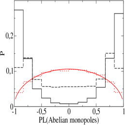
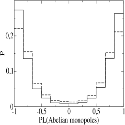
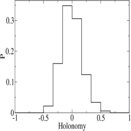
(a)                                                (b)                                                (c)

Figure 1: For confining configurations on a $20^{3}\times 6$ lattice at $\beta=2.3$ after $4D$ smearing, we show in: (a) the distribution of the Polyakov loop in lattice points where time-like Abelian monopole currents are present after 100 smearing steps (solid histogram for the Polyakov gauge, dashed histogram for MAG) compared with the overall distribution of the Polyakov loop (dotted histogram) which is well described by the Haar measure (solid curve). All distributions are normalized. (b) the distributions of the Polyakov loop in points where time-like Abelian monopole currents are present in Polyakov gauge comparing 100 and 50 smearing steps (solid and dashed histograms correspondingly). (c) the distribution of “asymptotic holonomy” (as defined in the text) after 100 smearing steps.

In Fig. 1b we compare the above mentioned distributions for lattice points with monopole currents (in the case of PG) obtained with respect to the number (100 and 50) of smearing steps. In order to facilitate a comparison of the clusters to analytical solutions with nontrivial holonomy, we define a so-called “asymptotic holonomy” for each lattice configuration. We consider the points on the lattice with the absolute value of topological charge density less than the averaged absolute value of topological charge density . We take the average of the Polyakov loop over this set of “asymptotic” points. The resulting distribution of the “asymptotic holonomy” $H$ for 500 smeared configurations (after 100 smearing steps) is shown in Fig. 1c. It can be seen from the last figure that the “asymptotic holonomy” $H$ is peaked at zero (understood as maximally nontrivial holonomy) and is still rather narrowly distributed. We will restrict further analysis to a subset of 330 smeared configurations with $|H|<1/6$, i.e. with maximally nontrivial holonomy.

III Cluster analysis of smeared configurations

For each of the $4D$ smeared configurations satisfying the cut $|H|<1/6$ we have looked for clusters of topological charge. The topological density is assigned to the lattice sites according to the plaquette definition. We take the points where the absolute value of the topological charge density exceeds some threshold value. This threshold has been varied between the average absolute value of the topological charge density and a value taken $10$ times larger. The link-connected points above the threshold value (below minus the threshold value) form what we call the positive (negative) clusters of topological charge. The precise threshold itself for each smeared configuration was chosen (within the above range) in such a way as to have the maximal number of disconnected clusters of topological charge for this configuration.

In this way we obtained $4684$ clusters, i.e. on average approximately 14 clusters per configuration. From these clusters we have selected $3464$ ($3107$) clusters that contain time-like Abelian monopole currents in PG (in MAG) as possible signatures for KvB monopole constituents. The remaining $1220$ ($1577$) clusters were free of time-like monopole currents. Although all clusters together occupy on average only $3.5\%$ of the 4-d volume they contain $39.5\%$ of the time-like Abelian monopole currents detected on the lattice.

Thus, time-like Abelian magnetic currents are about $18$ times more dense inside clusters of topological charge than outside. In order to select clusters containing either a single (more or less) static Abelian (anti)monopole, or monopole charges cancelling each other inside a topological cluster we determine an average monopole charge $~{}\overline{m}_{cluster}~{}$ for clusters containing timelike Abelian monopole currents. It is defined as the difference between the number of dual links with time-like currents going in the positive time direction (carrying positive magnetic charge) and the number of those with time-like currents going in the negative time direction (negative magnetic charge) divided by the total number of time-like monopole currents inside the cluster.

In $60\%$ of clusters with Abelian monopoles we observed only equal-sign monopole currents (i.e. all time-like Abelian monopole currents going in the same direction) resulting in $~{}\overline{m}_{cluster}=\pm 1$. On the other hand in approximately $8\%$ of clusters the numbers of positive and negative time-like Abelian monopole currents were equal to each other, i.e. $~{}\overline{m}_{cluster}=0$. Further, from the first group of clusters with $~{}\overline{m}_{cluster}=\pm 1~{}$ we have selected those with a number of time-like Abelian monopole currents larger than or equal to $N_{\tau}=6$ ($N_{\tau}$ is the number of time slices in the lattice), such that the Abelian monopole loop can close by periodicity in the time direction. Let us call them conditionally “static” clusters. In this way, finally, we have identified 547 (359) clusters with “conditionally static” monopoles in PG (MAG). Tentatively we labeled them as static dyons (eventually being part of a KvB caloron). The other 268 (638) clusters with a monopole-antimonopole pair are tentatively considered as undissociated KvB calorons.

In order to seek further support for this interpretation we have averaged the Polyakov loop inside the selected clusters over all points where time-like Abelian monopole currents of either sign are observed. We call this quantity the averaged Polyakov loop of the monopole “skeleton” of the given cluster, $\langle PL(\mathrm{Abelian~{}monopoles})\rangle_{cluster}$. From KvB calorons we expect this average for “static monopole clusters” ($~{}\overline{m}_{cluster}=\pm 1~{}$) to be close to $~{}\pm 1~{}$, whereas for “monopole-antimonopole pair clusters” ($~{}\overline{m}_{cluster}=0~{}$) it should be close to $~{}0~{}$, the latter because of the mentioned above dipole structure for the spatial Polyakov loop distribution inside the undissociated caloron. Indeed, the measured distributions of the Polyakov loop averaged over the monopole skeletons of the selected clusters are shown in Figs. 2 are peaking around $\pm 0.75$ for clusters classified as static dyons and around zero for clusters tentatively identified as undissociated KvB calorons. With fewer smearing steps the histogram for static dyons becomes less pronounced.

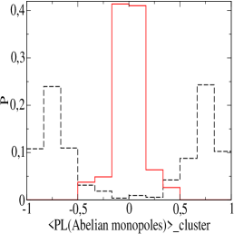
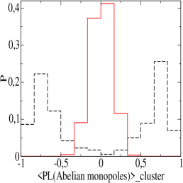
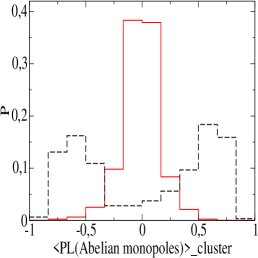
(a)                                                (b)                                                (c)

Figure 2: (a) The distribution of the Polyakov loop averaged over the monopole skeleton of topological clusters with static monopoles (dashed histogram) and for clusters with monopole-antimonopole pairs (solid histogram) (both according to the Polyakov gauge after 100 smearing steps). (b) The same for the maximally Abelian gauge and 100 smearing steps. (c) The same for the Polyakov gauge after only 50 smearing steps.

Next we would like to get some information also about the topological charge of objects tentatively identified as static dyons and undissociated KvB calorons. Since the clusters have been defined by means of a threshold for the density, some (uncertain) part of the cluster charge is residing in the tail of the density and has to be appended to the charge integral over the cluster. First we need some (model dependent) estimates for the actual size of the clusters of both kinds before we are able to define the total cluster charge by including the (observed) tail of the charge distribution as well. These estimates are different for the two types of clusters.

For a static dyon we know from the analytic KvB caloron solution that its size depends on the holonomy according to $~{}\bar{r}={b}/{4\pi\omega}~{}$ ($\omega~{}$ is the holonomy parameter, $H=\cos(2\pi\omega)$ and $b$ is the inverse temperature, the period in time direction). The topological charge density in the center, $q_{max}$, scales with the size in the following way:

$$q_{max}=\frac{1}{24\pi^{2}\bar{r}^{4}}~{}~{}.$$ (1)

(see the Appendix for some details). Fitting clusters classified as static dyons to this equation we can infer the cluster size from the observed maximum of the topological charge density inside the cluster. Then we sum the topological charge of all points that have a spatial distance from the point of maximum less than some radius $~{}R~{}$ related to $~{}\bar{r}$. This distance $~{}R~{}$ should not be too large in order to avoid double counting of topological charge density (by assigning points to more than one cluster) and not too small (in order not to underestimate the topological charge of the cluster considered). We use $R=3\bar{r}$ which would give for an isolated cluster (with an ideal, exponential profile of the topological charge density) the total charge within $7\%$ accuracy (there is no need to correct for the tail). In this way we assign a topological charge to all clusters classified as static dyon clusters.

An undissociated KvB caloron has a topological charge profile like that of an isolated ordinary instanton solution. For them the maximum of the topological charge density is related to the instanton size $~{}\rho~{}$ as follows (see Appendix)

$$q_{max}=\frac{6}{\pi^{2}\rho^{4}}~{}~{}.$$ (2)

Assuming that the clusters classified as undissociated calorons have this charge profile we can obtain the instanton size $~{}\rho~{}$ from the measured $~{}q_{max}~{}$ of the cluster. Then we sum the topological charge over all points that have a 4-dimensional distance less than $1.5\rho$ from the maximum position. The result needs to be multiplied by a correction factor $~{}1.29~{}$ as for the exact instanton solution (see Appendix). In this way we define an estimated topological charge also for clusters identified as undissociated calorons.

At this point we wish to explain why 100 smearing steps are more suitable than 50 for the detection of KvB dyons. Indeed, we will show later that the signal becomes more clear with more smearing steps. For an isolated dyon the topological density in the maximum is equal to $|q|_{max}=\pi^{2}/(24\times 6^{4})~{}~{}$ as it can be seen from Eq. (1) with $\omega=1/4$ (the case of maximally nontrivial holonomy) and $b=6$. Requiring the maximum of topological density in a cluster to exceed the threshold value (i.e. the averaged modulus of the topological density over the configuration), $|q|_{max}>\overline{|q|}$, we get an upper limit for $\overline{|q|}$ of a smeared configuration in order for an isolated dyon with maximally nontrivial holonomy to be recognized as a cluster by our cluster finding algorithm. This would give an action value $|q|_{max}\times 6\times 20^{3}\approx 15$ as an upper limit for the smeared action (given in instanton units). This value is close to the action of smeared configurations after 100 smearing steps as mentioned before.

As for the PG, we can present the two sorts of topological clusters ($547$ topological clusters seen after 100 smearing steps classified as static (anti)monopoles and $268$ clusters interpreted as monopole-antimonopole pairs) in a scatter plot with respect to the maximal value $~{}q_{max}~{}$ on one hand and the averaged Polyakov loop of the monopole skeleton ($\langle PL(\mathrm{Abelian~{}monopoles})\rangle_{cluster}$) on the other in Fig. 3a. The same for MAG is shown in Fig. 3b. The dependence on the number of smearing steps for the PG case can be concluded from Fig. 3c which refers to 50 smearing steps. The average size of single (anti)monopoles after 100 smearing steps is $~{}\bar{r}\approx(1\ldots 1.5)~{}a~{}$, whereas the most probable size of undissociated calorons is $~{}\rho\approx 3~{}a$ corresponding to a distance between constituents $d\approx 4.5~{}a$. The lattice spacing $~{}a~{}$ can be related to the deconfining temperature according to $~{}\beta=2.30\approx\beta_{c}(N_{\tau}=4)=2.29~{}$, resulting in $~{}a\approx 1/(4T_{c})$ . Less smearing results (on average) in a smaller size of both types of clusters (causing problems due to the finite resolution of the lattice).

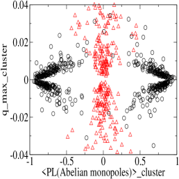
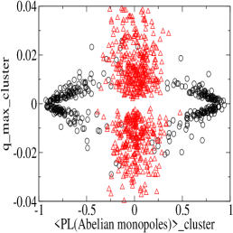
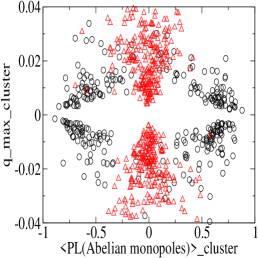
(a)                                                (b)                                                (c)

Figure 3: (a) The scatter plot shows the concentration of topological clusters after 100 smearing steps in the ${(q_{max})}_{cluster}$-$~{}\langle PL(\mathrm{Abelian~{}monopoles})\rangle_{cluster}$ plane, depending on the monopole content in the Polyakov gauge: clusters with static monopoles (circles) and clusters with monopole-antimonopole pairs (triangles) are forming different clusters in this plot. (b) The same for the maximally Abelian gauge. (c) The same for the Polyakov gauge after only 50 smearing steps.

The corresponding scatter plots with the estimated topological charge of each cluster $~{}Q_{cluster}~{}$ on one hand and the averaged Polyakov line of the monopole skeleton ($\langle PL(\mathrm{Abelian~{}monopoles})\rangle_{cluster}$) on the other are presented in Fig. 4. As it can be seen from this Figure the two sorts of topological clusters are clustering on the scatter plot either near the points $~{}\langle PL(\mathrm{Abelian~{}monopoles})\rangle_{cluster}=\pm 1,~{}Q_{cluster}=\pm 1/2~{}$ (dissociated) or $~{}\langle PL(\mathrm{Abelian~{}monopoles})\rangle_{cluster}=0,~{}Q_{cluster}=\pm 1~{}$ (undissociated).

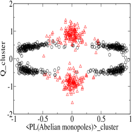
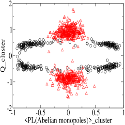
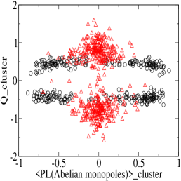
(a)                                                (b)                                                (c)

Figure 4: Scatter plots as in Figs. 3 (a), (b) and (c), respectively, but for the $Q_{cluster}$-$~{}\langle PL(\mathrm{Abelian~{}monopoles})\rangle_{cluster}$ plane.

The existence and interpretation of these two sorts of topological clusters can also be concluded from the corresponding reduced distributions shown on Fig. 2a and Fig. 5a focussing on $\langle PL(\mathrm{Abelian~{}monopoles})\rangle_{cluster}$ and $Q_{cluster}$, respectively, all for PG. Figs. 4b, 2b and 5b refer to MAG, while Figs. 4c, 2c and 5c describe PG after only 50 smearing steps, in order to demonstrate the effect of smearing.

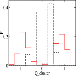
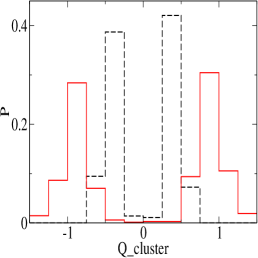
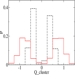
(a)                                                (b)                                                (c)

Figure 5: (a) The distribution of the topological charge per cluster, $Q_{cluster}$, of topological clusters after 100 smearing steps with static monopoles (dashed histogram) and for clusters with monopole-antimonopole pairs (solid histogram) in the Polyakov gauge. (b) The same for the maximally Abelian gauge. (c) The same for the Polyakov gauge after only 50 smearing steps.

That is what we expected for isolated dyons from KvB solutions in a background of maximally nontrivial holonomy and for undissociated KvB calorons in the same background. In order to check our picture we generated artificial topological clusters by discretizing analytical single KvB caloron solutions with maximally non-trivial holonomy also on a $20^{3}\times 6$ lattice. They were subjected to a few improved cooling steps in order to adapt them to the 3-dimensional periodicity of the lattice. The distance of the constituents was randomly varied from zero to the maximal possible value of $10\cdot\sqrt{3}$, in order to create both dissociated and non-dissociated calorons  We investigated these artificial clusters with the same instruments as described above. The results of this model calculation using MAG for detecting the Abelian monopoles are visualized in Figs. 6 and agree nicely with our findings before.

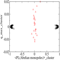
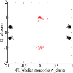
(a)                                               (b)

Figure 6: Scatter plots as in Figs. 3 and 4   but for $O(100)$ of artificially and randomly generated single caloron configurations. The monopole content is defined in the maximally Abelian gauge.

Thus, we can conclude to have found a clear signal (in smeared $SU(2)$ lattice configurations in the confining phase) of topological objects falling under the classification offered by extreme cases of the KvB solutions. One may wonder why only $~{}547+268=815~{}$ clusters (in PG) from $~{}4684~{}$ clusters in total are distinguished by their discernible monopole and topological content. It should be taken into account that the above signal could be clearly seen only for well isolated clusters, and we have selected clusters according to extreme cases of well separated constituents and instanton-like calorons. Generically, the clusters are just mutually disconnected, and there is no such clear relation between the maximal action density and the size of the cluster.

IV Conclusion

Investigating equilibrium lattice fields obtained at finite temperature in $SU(2)$ gluodynamics we have demonstrated that among the topological objects (observed in the confined phase after suitable smearing) there are both static dyons and nonstatic calorons. Static dyons are correlated with static Abelian monopoles obtained from Abelian projection in Polyakov gauge or maximally Abelian gauge. Nonstatic calorons are correlated with nonstatic loops of Abelian monopole-antimonopole pairs. The behaviour of the local Polyakov loop inside these objects and the (model-dependent) estimates of their topological charges favour the interpretation as KvB calorons with nontrivial holonomy, or as constituent dyons into which such KvB calorons can dissociate.

Appendix

The purpose of this appendix is to explain the method used to estimate the topological charge of objects first detected as clusters. The estimate depends on whether they have been classified as static dyons or undissociated KvB calorons.

Undissociated KvB calorons have an action profile like an ordinary instanton. For the latter the action density is equal to

$$s(x)=\frac{48\rho^{4}}{(x^{2}+\rho^{2})^{4}}~{}.$$ (3)

The value $~{}s(0)~{}$ normalized to the total instanton action of $~{}S_{inst}=8\pi^{2}~{}$ is presented in the text (see Eq. (2)). If one integrates the above action density over the 4-dimensional volume bounded by a sphere around the center with the radius $~{}1.5\rho~{}$ the result is equal to $~{}S_{inst}/1.29$. Therefore, in order to get the total action (topological charge) of an undissociated caloron we have to correct the above restricted integral (sum over lattice points) by the factor $~{}1.29$.

The other extreme case of an isolated dyon is more involved 0404210 . The action density for the general caloron solution with nontrivial holonomy is given by the following formulae KvB-1

$$s(x) = -\frac{1}{2}\partial^{2}_{\mu}\partial^{2}_{\nu}\log\psi(x)\,$$

$$\psi(x) = \cosh(4\pi r\omega)\cosh(4\pi s\bar{\omega})$$

$$+ \frac{(r^{2}\!+\!s^{2}\!+\!\pi^{2}\rho^{4})}{2rs}\sinh(4\pi r\omega)\sinh(4\pi s\bar{\omega})$$

$$+ \pi\rho^{2}\left(s^{-1}\sinh(4\pi s\bar{\omega})\cosh(4\pi r\omega)\right.$$

$$+\left.r^{-1}\sinh(4\pi r\omega)\cosh(4\pi s\bar{\omega})\right)$$

$$- \cos(2\pi t)~{},$$

where the period in time direction is set equal to $b=1$ (in other words, all distances are measured in $b$). The holonomy parameters $\omega$ and $\bar{\omega}$ are related to each other $\bar{\omega}=1/2-\omega,~{}~{}0\leq\omega\leq 1/2$. The distances $~{}r=|\vec{x}-\vec{x}_{1}|~{}$ and $~{}s=|\vec{x}-\vec{x}_{2}|~{}$ are the 3-dimensional distances from the locations of the two centers of the caloron solution. The distance between the centers $~{}d\equiv|\vec{x}_{1}-\vec{x}_{2}|~{}$ is connected with the scale size and the width of the time periodicity strip $~{}b~{}$ through

$$\pi\rho^{2}/b=d\,.$$ (5)

Now if we remove the second center (the dyon at $~{}\vec{x}_{2}~{}$) to infinity $~{}s\approx d\rightarrow\infty~{}$ we can find the potential $~{}\psi~{}$ for an isolated dyon, which obviously is static

$$\psi(x)=A\frac{\sinh(4\pi r\omega)}{r}~{},$$ (6)

where $~{}A~{}$ is some (infinite) constant not important for the calculation of the action density. Invoking the inverse temperature $~{}b~{}$ again, $~{}\bar{r}={b}/{4\pi\omega}~{}$ can be called the size of the dyon. In order to obtain the action density at the position $~{}\vec{x}_{1}~{}$ we expand $~{}\log\psi(x)~{}$ up to the fourth power in $~{}r~{}$

$$\log\psi(x)=A^{\prime}+\frac{1}{6}\frac{r^{2}}{\bar{r}^{2}}-\frac{1}{180}\frac{r^{4}}{\bar{r}^{4}}+...$$ (7)

and calculate the fourth derivative

$$s(\vec{x}_{1})=\frac{1}{3~{}\bar{r}^{4}}~{}.$$ (8)

Eq. (1) in the text is obtained by normalization of $~{}s(\vec{x}_{1})~{}$ to the total instanton action $~{}S_{inst}=8\pi^{2}$.

References

- (1)
- (2)
- (3) For a recent review see T. Schäfer and E. V. Shuryak, Rev. Mod. Phys. 70, 323 (1998).
- (4) I. Horvath et al., Phys. Rev. D66, 034501 (2002).
- (5) E.-M. Ilgenfritz et al., Nucl. Phys. B268, 693 (1986).
- (6) J. Hoek, M. Teper, and J. Waterhouse, Nucl. Phys. B288, 589 (1987).
- (7) M. I. Polikarpov and A. I. Veselov, Nucl. Phys. B297, 34 (1988).
- (8) P. de Forcrand, M. Garcia Perez, and I.-O. Stamatescu, Nucl. Phys. B499, 409 (1997).
- (9) T. DeGrand, A. Hasenfratz, and De-cai Zhu, Nucl. Phys. B475, 321 (1996); Nucl. Phys. B478, 349 (1996).
- (10) T. DeGrand, A. Hasenfratz, and T. G. Kovacs, Nucl. Phys. B505, 417 (1997).
- (11) M. Feurstein, E.-M. Ilgenfritz, M. Müller-Preussker, and S. Thurner, Nucl. Phys. B511, 421 (1998).
- (12) T. DeGrand, A. Hasenfratz, and T. G. Kovacs, Nucl. Phys. B520, 301 (1998).
- (13) T. C. Kraan and P. van Baal, Phys. Lett. B435, 389 (1998).
- (14) T. C. Kraan and P. van Baal, Nucl. Phys. B533, 627 (1998).
- (15) K. Lee and C. Lu, Phys. Rev. D58, 025011 (1998).
- (16) R. C. Brower et al., Nucl. Phys. Proc. Suppl. 73, 557 (1999).
- (17) D. Diakonov, Prog. Part. Nucl. Phys. 51, 173 (2003).
- (18) D. Diakonov, N. Gromov, V. Petrov, and S. Slizovskiy, Phys. Rev. D70, 036003 (2004).
- (19) E.-M. Ilgenfritz, B. V. Martemyanov, A. I. Veselov, M. Müller-Preussker, and S. Shcheredin, Phys. Rev. D66, 074503 (2002).
- (20) E.-M. Ilgenfritz, M. Müller-Preussker, B. V. Martemyanov, and A. I. Veselov, Phys. Rev. D69, 114505 (2004).
- (21) F. Bruckmann, E.-M. Ilgenfritz, B. V. Martemyanov, and P. van Baal, Phys. Rev. D70, 105013 (2004) .
- (22) See e.g. M. Engelhardt, plenary talk given at Latice 2004, e-Print Archive: hep-lat/0409023.
- (23) J. W. Negele, F. Lenz, and M. Thies, talk given at Lattice 2004, e-Print Archive: hep-lat/0409083.
- (24) C. Gattringer and S. Schaefer, Nucl. Phys. B654, 30 (2003).
- (25) C. Gattringer et al., talks by C. Gattringer and E.-M. Ilgenfritz at Lattice 2003, Nucl. Phys. Proc. Suppl. 129, 653 (2004).
- (26) D. Peschka, E.-M. Ilgenfritz, and M. Müller-Preussker, in preparation.
- (27) V. Bornyakov and G. Schierholz, Phys. Lett. B384, 190 (1996).
- (28) H. Markum, W. Sakuler, and S. Thurner, Nucl. Phys. Proc. Suppl. 47, 254 (1996).
- (29) E.-M. Ilgenfritz, H. Markum, M. Müller-Preussker, and S. Thurner, Phys. Rev. D58, 094502 (1998).
- (30) M. N. Chernodub, F. V. Gubarev, and M. I. Polikarpov, Nucl. Phys. Proc. Suppl. 63, 516 (1998); JETP Letters 69, 169 (1999).
- (31) T. A. DeGrand and D. Toussaint, Phys. Rev. D22, 2478 (1980).
- (32) G. ’t Hooft, Nucl. Phys. B190, 455 (1981).
- (33) A. S. Kronfeld, G. Schierholz, and U. J. Wiese, Nucl. Phys. B293, 461 (1987); A. S. Kronfeld, M. L. Laursen, G. Schierholz, and U. J. Wiese, Phys. Lett. B198, 516 (1987).
- (34) see also: F. Bruckmann, D. Nogradi, and P. van Baal, Nucl. Phys. B698, 233 (2004).