Anisotropic lattice with nonperturbative accuracy

Abstract

We determine the nonperturbative anisotropic parameter of the gauge action in the quenched approximation with less than 1% accuracy using the Sommer scale measured by the Lüscher-Weisz algorithm or smearing technique. We also study the nonperturbative O(a)-improvement of the quark action. The bare quark anisotropy is determined using the masses from the temporal and spatial directions. For the determination of the $O(a)$ improvement coefficients, we apply the Schrödinger functional method.

1 Introduction

Anisotropic lattices whose temporal lattice spacing $a_{\tau}$ is finer than the spatial one $a_{\sigma}$ have become a powerful tool in various subjects of lattice QCD simulations. Among these applications, computations of heavy-light matrix elements [1, 2, 3, 4] require the most accurate parameter tuning, which should be performed nonperturbatively. In this paper, we report the status of our project to develop the anisotropic lattice framework for such precision computations with accuracy of a few percent level [5].

Here we briefly summarize our strategy. For precise computations of heavy-light matrix elements, we need a framework of the heavy quark in which one should be able to (i) take the continuum limit, (ii) compute the parameters in the action and the operators nonperturbatively, (iii) and compute the matrix elements with a modest computational cost. The anisotropic lattice is a candidate of such framework, if a method which fulfills the above condition (ii) is provided. Our expectation is that on anisotropic lattices the mass dependence of the parameters becomes so mild that one can adopt coefficients determined nonperturbatively at massless limit. We also need to control all the systematic errors in the continuum extrapolations. Feasibility studies performed so far for the level of $O(10\%)$ computations are encouraging for further development [3, 4]. We therefore investigate calibration procedures at the accuracy less than one percent, both for the gauge and quark actions in the quenched approximation at $\xi=4$ [5].

2 Calibration of gauge field

To achieve a few percent accuracy in the final results, the tuning of parameters must be performed at much less than this accuracy. As the goal of present work, we intend to determine the anisotropy parameters at $O(0.2\%)$ level. The elaborated work by Klassen [6], the $O(1\%)$ level calibration for the Wilson action, is therefore no longer meets the present condition. For more precise calibration of the gauge field, we need to measure the static quark potential very accurately. For this purpose, we adopt the Lüscher-Weisz noise reduction technique [9] as well as the standard smearing technique while applied in the anisotropic plane. The former method can drastically reduce the statistical errors while requires larger memory resources than the latter.

We define the renormalized anisotropy $\xi_{G}$ through the hadronic radii $r_{0}$ measured in the coarse and fine directions. Since we carry out the continuum extrapolation in terms of the lattice scale set by $r_{0}$, the renormalized anisotropy is kept fixed during the extrapolation. This avoids the systematic uncertainties due to the anisotropy which may remain in the continuum limit.

Figure 1 shows a result of calibration at $\beta=5.75$. The top panel shows the result for the static potential determined with the Lüscher-Weisz technique at $\gamma_{G}=3.072$. The renormalized anisotropy $\xi_{G}$ is determined with 0.2% accuracy. A linear fit of the results at several values of $\gamma_{G}$ determines $\gamma_{G}^{*}$ for which $\xi_{G}=4$ holds with 0.2% accuracy as displayed in the bottom panel.

Figure 1: Determination of the gauge field anisotropy at $\beta=5.75$.

In Figure 2, the results at several values of $\beta$ are collected. Although the precisions of the result with potential determined with the standard smearing technique are still not enough, sufficient precision is achieved at $\beta\leq 6$ where we used the L-W method. Improvement of calculation at $\beta>6$ and global fit analysis are in progress.

Figure 2: Result of calibration of gauge field.

3 Calibration of quark field

Our heavy quark formulation basically follows the Fermilab approach [7] but is formulated on the anisotropic lattices [1, 8]. The quark action is represented as

$$S_{F} = \sum_{x,y}\bar{\psi}(x)K(x,y)\psi(y),$$ (1)

$$K(x,y)\!\!\! = \!\!\!\delta_{x,y}-\kappa_{\tau}\left[\ \ (1-\gamma_{4})U_{4}(x)\delta_{x+\hat{4},y}\right.$$ (2)

$$\hskip 28.45274pt+\left.(1+\gamma_{4})U_{4}^{{\dagger}}(x-\hat{4})\delta_{x-\hat{4},y}\right]$$

$$-\kappa_{\sigma}{\textstyle\sum_{i}}\left[\ \ (r-\gamma_{i})U_{i}(x)\delta_{x+\hat{i},y}\right.$$

$$\hskip 28.45274pt+\left.(r+\gamma_{i})U_{i}^{{\dagger}}(x-\hat{i})\delta_{x-\hat{i},y}\right]$$

$$-\kappa_{\sigma}c_{E}{\textstyle\sum_{i}}\sigma_{4i}F_{4i}(x)\delta_{x,y}$$

$$-r\kappa_{\sigma}c_{B}{\textstyle\sum_{i>j}}\sigma_{ij}F_{ij}(x)\delta_{x,y},$$

where $\kappa_{\sigma}$ and $\kappa_{\tau}$ are the spatial and temporal hopping parameters, $r$ the spatial Wilson parameter and $c_{E}$ and $c_{B}$ the clover coefficients. For a given $\kappa_{\sigma}$, in principle, the four parameters $\gamma_{F}\equiv\kappa_{\tau}/\kappa_{\sigma}$, $r$, $c_{E}$ and $c_{B}$ should be tuned. We can set $r=1/\xi$ without loss of generality [1, 7].

Figure 3: Tuning of $c_{E}$ at $\beta=6.1$.

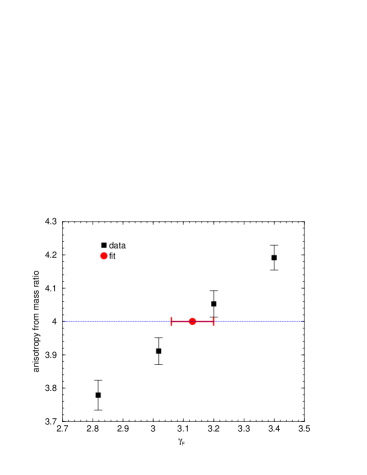
Figure 4: Determination of $\gamma_{F}^{*}$ at $\beta=5.75$.

We must calibrate $\gamma_{F}$, $c_{E}$, and $c_{B}$ to the level which enables computations of matrix elements within a few percent accuracy. We also need to perform the nonperturbative renormalization of the operators such as the heavy-light axial current. The nonperturbative renormalization technique [10] is one of the most powerful methods to perform such a program. Following our strategy, this technique can also be applied with a little modification for the anisotropic lattice.

We perform the calibration of $\gamma_{F}$, $c_{E}$, $c_{B}$, and the renormalization coefficients of the axial current along the following steps. (1) Tuning of $c_{E}$ by Schrödinger functional method. (2) Calibration of $\gamma_{F}$ (and $c_{B}$ if possible) by requiring the physical isotropy conditions for $m_{PS}$ and $m_{V}$ in the coarse and fine directions on lattices with $T$,$L$ $\stackrel{{\scriptstyle>}}{{\scriptstyle\sim}}$ 2 fm. (3) Determination of $c_{B}$, $\kappa_{c}$ and the renormalization coefficients of the axial current by Schrödinger functional method. We also need to verify that the systematic errors are under control by calculating the hadron spectra and the dispersion relations and by taking the continuum limit. It is also necessary to verify that the tuned parameters in the massless limit is also available in the heavy quark mass region.

To verify the feasibility of the step (1), we determine $c_{E}$ with fixed values of $\gamma_{F}$ and $c_{B}$. At $\beta=9.5$, the method is successfully applicable, and the result for $c_{E}$ is close to the 1-loop mean-field value. Figure 3 shows the result at $\beta=6.1$ ($a_{\sigma}\simeq 2$ GeV). The tuned value of $c_{E}$ is obtained as the value at which $\Delta M$, the difference of the quark mass defined through the axial Ward identity under different kinematical conditions, vanishes up to $O(a^{2})$ effects. The result of $c_{E}$ is larger than the tadpole improved tree level value. It is also found that $\Delta M$ is not sensitive to the change of $c_{B}$.

Figure 4 shows the result for the step (2) at $\beta=5.75$ on a $12^{2}\times 24\times 96$ lattice. The values of $\xi_{F}$ is determined from the meson masses in the fine and coarse directions. We note that the result for $\gamma_{F}^{*}$ is consistent with that from the dispersion relation [2]. At this stage, the precision of $\gamma_{F}^{*}$ is still not sufficient, while several techniques to reduce the statistical noise are yet to be tested. For the determination of $c_{B}$, the ratio of the hyperfine splittings in the fine and coarse directions is not feasible because of large statistical noise. Other procedures, such as Schrödinger functional method with boundaries in the coarse direction, are under investigation.

References

- [1] J. Harada et al., Phys. Rev. D 64 (2001) 074501.
- [2] H. Matsufuru, T. Onogi and T. Umeda, Phys. Rev. D 64 (2001) 114503.
- [3] J. Harada, H. Matsufuru, T. Onogi and A. Sugita, Phys. Rev. D 66 (2002) 014509.
- [4] H. Matsufuru et al., Nucl. Phys. B (Proc. Suppl.) 119 (2003) 601.
- [5] H. Matsufuru et al., Nucl. Phys. B (Proc. Suppl.) 129 (2004) 370.
- [6] T. R. Klassen, Nucl. Phys. B 533 (1998) 557.
- [7] A. X. El-Khadra, A. S. Kronfeld and P. B. Mackenzie, Phys. Rev. D 55 (1997) 3933.
- [8] T. Umeda et al., Int. J. Mod. Phys. A 16 (2001) 2215.
- [9] M. Lüscher and P. Weisz, JHEP 0109 (2001) 010.
- [10] M. Lüscher et al., Nucl. Phys. B478 (1996) 365; Nucl. Phys. B491 (1997) 323.