DESY 04-213, FTUV-04-1106, IFIC/04-66,
INT-Pub 04-29, LPT-Orsay/04-114, NT@UW-04-025,
ROMA-1392/04, RM3-TH/04-23, SHEP 0434, UW/PT 04-22

An exploratory lattice study of $\Delta I=3/2$ $K\rightarrow\pi\pi$ decays at next-to-leading order in the chiral expansion

Philippe Boucaud^a, Vicent Giménez^b, C.-J. David Lin^c, Vittorio Lubicz^d, Guido Martinelli^e, Mauro Papinutto^f, Chris T. Sachrajda^g

^a Université de Paris Sud, LPT (Bât. 210), Centre d’Orsay, 91405 Orsay-Cedex, France
^b Dep. de Física Teòrica and IFIC, Univ. de València, Dr. Moliner 50, E-46100, Burjassot, València, Spain
^c Department of Physics, University of Washington, Seattle, WA-98195-1550, USA & Institute for Nuclear Theory, University of Washington, Seattle, WA-98195-1560, USA
^d Dipartimento di Fisica, Universitá di Roma Tre and INFN, Sezione di Roma III,
Via della Vasca Navale 84, I-00146 Roma, Italy
^e Dipartimento di Fisica, Universitá di Roma “La Sapienza” and
INFN, Sezione di Roma, P.le A. Moro 2, I-00185 Roma, Italy
^f NIC/DESY Zeuthen, Platanenalle 6, D-15738 Zeuthen, Germany
^g School of Physics and Astronomy, University of Southampton,
Southampton SO17 1BJ, England

We present the first direct evaluation of $\Delta I=3/2$ $K\rightarrow\pi\pi$ matrix elements with the aim of determining all the low-energy constants at NLO in the chiral expansion. Our numerical investigation demonstrates that it is indeed possible to determine the $K\to\pi\pi$ matrix elements directly for the masses and momenta used in the simulation with good precision. In this range however, we find that the matrix elements do not satisfy the predictions of NLO chiral perturbation theory. For the chiral extrapolation we therefore use a hybrid procedure which combines the observed polynomial behaviour in masses and momenta of our lattice results, with NLO chiral perturbation theory at lower masses. In this way we find stable results for the quenched matrix elements of the electroweak penguin operators (${}_{I=2}\langle\pi\pi|{\mathcal{O}}_{8}|K^{0}\rangle=(0.68\pm 0.09)\mbox{ GeV}^{3}$ and ${}_{I=2}\langle\pi\pi|{\mathcal{O}}_{7}|K^{0}\rangle=(0.12\pm 0.02)\mbox{ GeV}^{3}$ in the NDR-$\overline{\textrm{MS}}$ scheme at the scale 2 GeV), but not for the matrix elements of ${\cal O}_{4}$ (for which there are too many Low-Energy Constants at NLO for a reliable extrapolation). For all three operators we find that the effect of including the NLO corrections is significant (typically about 30%). We present a detailed discussion of the status of the prospects for the reduction of the systematic uncertainties.

1 Introduction

The importance of a theoretical understanding of $K\to\pi\pi$ decays is underlined by the recent measurements of a non-zero value for the $\varepsilon^{\prime}/\varepsilon$ parameter [1, 2] (the first confirmed observation of direct CP violation) as well as the long-standing puzzle of the $\Delta I=1/2$ rule. Within the Standard Model of particle physics, the major difficulty is to quantify the non-perturbative QCD effects. Lattice simulations are being used in attempts to overcome this problem, but the results obtained in this way currently have large systematic errors. A major source of uncertainty is induced by the chiral extrapolation. Lattice simulations are performed with $u$- and $d$-quark masses typically in the range $m_{s}/2\leq m_{u,d}\leq m_{s}$ (where $m_{s}$ is the strange-quark mass), and the physical amplitudes are obtained by combining the lattice measurements with Chiral Perturbation Theory ($\chi$PT). Previous calculations of $K\to\pi\pi$ matrix elements were performed at leading-order (LO) in the chiral expansion. Following some early attempts to evaluate $K\to\pi\pi$ matrix elements directly [3, 4, 5, 6], lattice estimates of the $\Delta I=3/2$ $K\to\pi\pi$ matrix elements $\langle\pi^{+}\pi^{0}|{\mathcal{O}}^{3/2}_{7,8}|K^{+}\rangle$ [7, 8, 9, 10, 11] have generally been obtained by calculating the $K\to\pi$ matrix elements $\langle\pi^{+}|{\mathcal{O}}^{3/2}_{7,8}|K^{+}\rangle$ and using the soft-pion theorem $(-i)\langle\pi|{\mathcal{O}}|K\rangle/f_{\pi}\sim\langle\pi\pi|{\mathcal{O}}|K\rangle$ [12]. An exception to this has been the computation of the $K\to\pi\pi$ matrix element of the operator ${\cal O}_{+}$ (defined in eq. (4) below), with all three mesons at rest [13].

We have previously proposed improving the precision of lattice determinations of the decay amplitudes by computing directly $K\to\pi\pi$ matrix elements at unphysical kinematics and combining them with $\chi$PT at next-to-leading order (NLO) [14, 15]. By comparing the behaviour of the computed matrix elements as functions of the mesons’ masses and momenta with the predictions of chiral perturbation theory at NLO, we can, at least in principle, determine the low-energy constants and hence evaluate the physical amplitudes. In this paper we perform an exploratory numerical study to investigate the extent to which such a programme can be carried out in practice. In particular, we evaluate the matrix elements $\langle\pi^{+}\pi^{0}|{\mathcal{O}}_{i}|K^{+}\rangle$ for the following $\Delta I=3/2$ operators ${\mathcal{O}}_{i}$:

$${\mathcal{O}}_{4} = (\bar{s}_{\alpha}d_{\alpha})_{L}\left[(\bar{u}_{\beta}u_{\beta})_{L}-(\bar{d}_{\beta}d_{\beta})_{L}\right]+(\bar{s}_{\alpha}u_{\alpha})_{L}(\bar{u}_{\beta}d_{\beta})_{L},$$ (1)

$${\mathcal{O}}^{3/2}_{7} = (\bar{s}_{\alpha}d_{\alpha})_{L}\left[(\bar{u}_{\beta}u_{\beta})_{R}-(\bar{d}_{\beta}d_{\beta})_{R}\right]+(\bar{s}_{\alpha}u_{\alpha})_{L}(\bar{u}_{\beta}d_{\beta})_{R},$$ (2)

$${\mathcal{O}}^{3/2}_{8} = (\bar{s}_{\alpha}d_{\beta})_{L}\left[(\bar{u}_{\beta}u_{\alpha})_{R}-(\bar{d}_{\beta}d_{\alpha})_{R}\right]+(\bar{s}_{\alpha}u_{\beta})_{L}(\bar{u}_{\beta}d_{\alpha})_{R},$$ (3)

where $\alpha$ and $\beta$ are colour indices and $(\bar{\psi}_{1}\psi_{2})_{L,R}=\bar{\psi}_{1}\gamma_{\mu}(1\mp\gamma_{5})\psi_{2}$.

The matrix elements of the $\Delta I=3/2$ operator ${\mathcal{O}}_{4}$, first introduced in ref. [16], give dominant contributions to CP-conserving $K\rightarrow\pi\pi$ decays. ${\mathcal{O}}_{4}$ is proportional to the $\Delta I=3/2$ component of the operator

$${\mathcal{O}}_{+}=\frac{1}{2}\left[\left(\bar{s}_{\alpha}d_{\alpha}\right)_{L}\left(\bar{u}_{\alpha}u_{\alpha}\right)_{L}+\left(\bar{s}_{\alpha}u_{\alpha}\right)_{L}\left(\bar{u}_{\alpha}d_{\alpha}\right)_{L}\right],$$ (4)

whose matrix element, $\langle\pi^{+}\pi^{0}|{\mathcal{O}}_{+}|K^{+}\rangle=\langle\pi^{+}\pi^{0}|{\mathcal{O}}_{4}|K^{+}\rangle/3$, is an important theoretical input to the study of the $\Delta I=1/2$ rule. A consequence of chiral symmetry is that this matrix element can be related to $\langle K^{0}|(\bar{s}d)_{L}(\bar{s}d)_{L}|\bar{K}^{0}\rangle$ [17], which contains the non-perturbative QCD effects in $K^{0}{-}\bar{K}^{0}$ mixing (i.e. the two matrix elements are given in terms of the same low-energy constants).

${\mathcal{O}}^{3/2}_{7}$ and ${\mathcal{O}}^{3/2}_{8}$ are proportional to the $\Delta I=3/2$ component of the electroweak penguin operators,

$${\mathcal{O}}_{7}=\frac{3}{2}(\bar{s}_{\alpha}d_{\alpha})_{L}\sum_{q}e_{q}(\bar{q}_{\beta}q_{\beta})_{R}\qquad\textrm{and}\qquad{\mathcal{O}}_{8}=\frac{3}{2}(\bar{s}_{\alpha}d_{\beta})_{L}\sum_{q}e_{q}(\bar{q}_{\beta}q_{\alpha})_{R}\ .$$ (5)

These operators, although suppressed by a factor of $\alpha_{\mathrm{em}}/\alpha_{s}$ compared to QCD penguin operators, can contribute significantly in the theoretical prediction of $\varepsilon^{\prime}/\varepsilon$ [18, 19]. Recent estimates [20, 21, 22, 23, 24] suggest that ${\mathcal{O}}_{8}$ has a significant negative contribution to $\varepsilon^{\prime}/\varepsilon$.

In principle, by using finite-volume techniques, it is possible to calculate $K\rightarrow\pi\pi$ amplitudes directly from lattice QCD [25, 26], without using chiral perturbation theory. However, in order to obtain the physical amplitude from simulations with periodic boundary conditions for the fields, one requires lattice sizes of order 6 fm or larger, which is numerically very demanding . In addition for $\Delta I=1/2$ decays, the lack of unitarity and enhanced long-distance effects in quenched and partially quenched QCD suggest that one needs to use full QCD to determine these matrix elements [29, 30, 31]. This problem is much less severe for the $\Delta I=3/2$ decays studied in this paper. For matrix elements as complicated as those contributing to $K\to\pi\pi$ decay amplitudes, unquenched simulations on sufficiently large volumes and on fine lattices are unlikely in the near future. It will therefore continue to be necessary to combine $\chi$PT with lattice simulations for the foreseeable future.

In this paper we present the first lattice study of the matrix elements $\langle\pi^{+}\pi^{0}|{\mathcal{O}}_{i}|K^{+}\rangle$ (${\mathcal{O}}_{i}={\mathcal{O}}_{4},{\mathcal{O}}^{3/2}_{7,8}$) at next-to-leading order (NLO) in the chiral expansion. We follow the strategy proposed in refs. [14, 15]. Under the $SU(3)_{\mathrm{L}}\times SU(3)_{\mathrm{R}}$ flavour transformation, the operator ${\mathcal{O}}_{4}$ is in the $(27_{\mathrm{L}},1_{\mathrm{R}})$ irreducible representation and ${\mathcal{O}}_{7,8}$ (and hence ${\mathcal{O}}^{3/2}_{7,8}$) are in the $(8_{\mathrm{L}},8_{\mathrm{R}})$ irreducible representation. This means that the chiral expansion for the matrix elements of ${\mathcal{O}}_{4}$ starts at ${\mathcal{O}}(p^{2})$, while that for ${\mathcal{O}}_{7,8}$ and ${\mathcal{O}}^{3/2}_{7,8}$ starts at ${\mathcal{O}}(p^{0})$. In sec. 2 we recall the demonstration that by allowing one of the pions to carry non-zero spatial momentum we are able, in principle at least, to determine these matrix elements at NLO in the chiral expansion [14, 15].

Although we were able to determine the matrix elements $\langle\pi^{+}\pi^{0}|{\mathcal{O}}_{4}|K^{+}\rangle$ at the quark masses at which the simulations were performed, we were unable to perform the chiral extrapolation with any degree of confidence. For this matrix element there is one low-energy constant at lowest order and six more at NLO and it was not possible to determine so many parameters with sufficient precision by using our lattice data. Nevertheless, our study already reveals some qualitative feature of this matrix element, which will be discussed in detail in sec. 5. For $\langle\pi^{+}\pi^{0}|{\mathcal{O}}^{3/2}_{7,8}|K^{+}\rangle$ there are fewer low-energy constants and we were able to estimate the physical matrix elements. Our best estimates for these matrix elements renormalized in the NDR-$\overline{\mbox{MS}}$ scheme at $2\mbox{ GeV}$ are (see sec. 7),

$${}_{I=2}\langle\pi\pi|{\mathcal{O}}_{8}|K^{0}\rangle^{\textrm{\scriptsize{NLO}}}_{\textrm{\scriptsize{phys}}} = 0.68\,(6)\,(4)\,(5)\mbox{ GeV}^{3}$$

$${}_{I=2}\langle\pi\pi|{\mathcal{O}}_{7}|K^{0}\rangle^{\textrm{\scriptsize{NLO}}}_{\textrm{\scriptsize{phys}}} = 0.12\,(1)\,(1)\,(1)\mbox{ GeV}^{3}\,.$$ (6)

The first error is statistical, the second is due to the uncertainties in the non-perturbative matching to the continuum renormalization scheme and the third is due to the chiral extrapolations. In addition to the errors quoted above, there are uncertainties due to quenching, possible scaling violations and finite-volume effects which are more difficult to estimate reliably. We discuss these in sec. 6.

The plan for the remainder of the paper is as follows. In the next section we explain our strategy for the determination of all the low-energy constants which are required for the evaluation of the physical amplitudes at NLO in the chiral expansion. The parameters and details of our simulation are presented in sec. 3. In sec. 4 we explain our procedure for the non-perturbative renormalization of the lattice operators. The details of our analysis and a discussion of the systematic uncertainties are presented in secs. 5 and 6 respectively. Section 7 contains the main numerical results of this study and a comparison with those from previous calculations. Preliminary reports on this work have been presented in refs. [32, 33]. We present our conclusions in sec. 8. There is one appendix in which we study the chiral behaviour of the $K\to\pi$ matrix elements obtained by the CP-PACS collaboration [11] and argue that different choices of ansatz for the chiral extrapolation can lead to significantly different results.

2 Strategy for the Determination of the Physical Amplitudes

In this study we follow the strategy presented in refs. [14, 15] for the determination of the physical amplitudes from lattice simulations combined with $\chi$PT at NLO. In order to be able to extract all the low-energy constants at NLO, we must evaluate $K\to\pi\pi$ matrix elements for a range of unphysical masses and momenta. We choose to use the SPQR kinematics, in which one of the final-state pions has a non-zero spatial momentum and the other two mesons are at rest.

The chiral expansion for the matrix elements ${\mathcal{M}}^{(4)}_{\mathrm{SPQR}}\equiv\langle\pi^{+}\pi^{0}|{\mathcal{O}}_{4}|K^{+}\rangle$ and ${\mathcal{M}}^{(7,8)}_{\mathrm{SPQR}}\equiv\langle\pi^{+}\pi^{0}|{\mathcal{O}}^{3/2}_{7,8}|K^{+}\rangle$ in the SPQR kinematics, to NLO and in infinite volume is:

$${\mathcal{M}}^{(4)}_{\mathrm{SPQR}} = -\frac{6\sqrt{2}}{f_{K}\,f_{\pi}^{2}}\Bigg{\{}\alpha\Big{(}E_{\pi}M_{\pi}+\frac{1}{2}M_{K}\,(E_{\pi}+M_{\pi})+[\textrm{chiral logs}]^{(4)}_{\mathrm{SPQR}}\Big{)}$$ (7)

$$+4\beta_{2}M^{4}_{\pi}+(4\beta_{4}+2\beta_{7})E_{\pi}M^{3}_{\pi}+(\beta_{4}-\beta_{5}+\beta_{7})M^{3}_{\pi}M_{K}$$

$$+(\beta_{4}-\beta_{5}+\beta_{7}+2\beta_{22})E_{\pi}M^{2}_{\pi}M_{K}+(-4\beta_{2}+8\beta_{24})M^{2}_{\pi}M^{2}_{K}+(\beta_{4}+2\beta_{7})E_{\pi}M^{3}_{K}$$

$$+(-2\beta_{5}+4\beta_{7}+4\beta_{22})E_{\pi}M_{\pi}M^{2}_{K}+(\beta_{4}+2\beta_{7})M_{\pi}M^{3}_{K}$$

$$+(-16\beta_{24})E^{2}_{\pi}M^{2}_{\pi}+2\beta_{22}E^{2}_{\pi}M_{\pi}M_{K}+8\beta_{24}E^{2}_{\pi}M^{2}_{K}\,\Bigg{\}}\,$$

$$= -\frac{6\sqrt{2}}{f^{3}}\Bigg{\{}$$

$$\alpha\Big{\{}\Big{[}E_{\pi}M_{\pi}+\frac{1}{2}M_{K}\,(E_{\pi}+M_{\pi})\Big{]}[\textrm{chiral logs}]_{f^{3}}(M_{\pi},M_{K})+[\textrm{chiral logs}]^{(4)}_{\mathrm{SPQR}}\Big{\}}$$

$$+4\beta_{2}M^{4}_{\pi}+\left(4\beta_{4}+2\beta_{7}-\frac{24L_{4}}{f^{2}}-\frac{16L_{5}}{f^{2}}\right)E_{\pi}M^{3}_{\pi}$$

$$+\left(\beta_{4}-\beta_{5}+\beta_{7}-\frac{12L_{4}}{f^{2}}-\frac{8L_{5}}{f^{2}}\right)M^{3}_{\pi}M_{K}$$

$$+\left(\beta_{4}-\beta_{5}+\beta_{7}+2\beta_{22}-\frac{12L_{4}}{f^{2}}-\frac{8L_{5}}{f^{2}}\right)E_{\pi}M^{2}_{\pi}M_{K}+(-4\beta_{2}+8\beta_{24})M^{2}_{\pi}M^{2}_{K}$$

$$+\left(\beta_{4}+2\beta_{7}-\frac{24L_{4}}{f^{2}}-\frac{4L_{5}}{f^{2}}\right)E_{\pi}M^{3}_{K}$$

$$+\left(-2\beta_{5}+4\beta_{7}+4\beta_{22}-\frac{48L_{4}}{f^{2}}-\frac{8L_{5}}{f^{2}}\right)E_{\pi}M_{\pi}M^{2}_{K}$$

$$+\left(\beta_{4}+2\beta_{7}-\frac{24L_{4}}{f^{2}}-\frac{4L_{5}}{f^{2}}\right)M_{\pi}M^{3}_{K}$$

$$+(-16\beta_{24})E^{2}_{\pi}M^{2}_{\pi}+2\beta_{22}E^{2}_{\pi}M_{\pi}M_{K}+8\beta_{24}E^{2}_{\pi}M^{2}_{K}\,\Bigg{\}}\,,$$

$${\mathcal{M}}^{(7,8)}_{\mathrm{SPQR}} = \frac{4\sqrt{2}}{f_{K}\,f_{\pi}^{2}}\,\Bigg{\{}\gamma^{(7,8)}\,(1+[\textrm{chiral logs}]^{\mathrm{EWP}}_{\mathrm{SPQR}})+2\Big{(}\delta^{(7,8)}_{4}+\delta^{(7,8)}_{5}+2\delta^{(7,8)}_{6}\Big{)}\,M_{K}^{2}$$ (8)

$$+\frac{1}{2}\Big{(}\delta^{(7,8)}_{1}-\delta^{(7,8)}_{2}-2\delta^{(7,8)}_{3}\Big{)}(M_{\pi}+E_{\pi})M_{K}$$

$$+2\Big{(}2(\delta^{(7,8)}_{4}+\delta^{(7,8)}_{5})+\delta^{(7,8)}_{6}\Big{)}M_{\pi}^{2}-\Big{(}\delta^{(7,8)}_{1}+\delta^{(7,8)}_{2}\Big{)}M_{\pi}E_{\pi}\Bigg{\}}$$

$$= \frac{4\sqrt{2}}{f^{3}}\,\Bigg{\{}\gamma^{(7,8)}\,\Big{(}1+[\textrm{chiral logs}]^{\mathrm{EWP}}_{\mathrm{SPQR}}+[\textrm{chiral logs}]_{f^{3}}(M_{\pi},M_{K})\Big{)}$$

$$+2\Big{(}\delta^{(7,8)}_{4}+\delta^{(7,8)}_{5}+2\delta^{(7,8)}_{6}-\frac{24L_{4}}{f^{2}}-\frac{4L_{5}}{f^{2}}\Big{)}\,M_{K}^{2}$$

$$+\frac{1}{2}\Big{(}\delta^{(7,8)}_{1}-\delta^{(7,8)}_{2}-2\delta^{(7,8)}_{3}\Big{)}(M_{\pi}+E_{\pi})M_{K}$$

$$+2\Big{(}2(\delta^{(7,8)}_{4}+\delta^{(7,8)}_{5})+\delta^{(7,8)}_{6}-\frac{12L_{4}}{f^{2}}-\frac{8L_{5}}{f^{2}}\Big{)}M_{\pi}^{2}-\Big{(}\delta^{(7,8)}_{1}+\delta^{(7,8)}_{2}\Big{)}M_{\pi}E_{\pi}\Bigg{\}}\,,$$

where $[\textrm{chiral logs}]^{(4)}_{\mathrm{SPQR}}$ and $[\textrm{chiral logs}]^{\mathrm{EWP}}_{\mathrm{SPQR}}$ are calculated in [15] in both full QCD and quenched QCD (qQCD). With the exception of $f$, which is the pseudoscalar decay constant in the chiral limit , the quantities appearing in eqs. (7) and (8) all correspond to the masses and energies used in the simulations ($M_{\pi}$ is the pion mass, $M_{K}$ the kaon mass and $E_{\pi}$ the energy of the pion with non-zero spatial momentum). All dimensionful quantities are taken to be in lattice units. $\alpha$, $\beta_{i}$, $\gamma^{(7,8)}$ and $\delta^{(7,8)}_{i}$ are the unknown low-energy constants (LECs) in the chiral expansion for these weak amplitudes. $L_{4,5}$ are the standard Gasser-Leutwyler constants in the strong chiral Lagrangian [34]. $[\textrm{chiral logs}]_{f^{3}}$ represents the chiral logarithms appearing in the renormalization of the factor $1/f_{K}f_{\pi}^{2}$ and are known for both QCD and qQCD [34, 35].

The chiral expansion for the physical matrix elements, ${\mathcal{M}}^{(4,7,8)}_{\mathrm{phys}}$ (that is $\langle\pi^{+}\pi^{0}|{\mathcal{O}}_{4}|K^{+}\rangle$ and $\langle\pi^{+}\pi^{0}|{\mathcal{O}}^{3/2}_{7,8}|K^{+}\rangle$ with the four-momenta of the initial and final states equal), to NLO in infinite volume is:

$${\mathcal{M}}^{(4)}_{\mathrm{phys}} = -\frac{6\sqrt{2}}{f_{K}\,f_{\pi}^{2}}\Bigg{\{}\alpha\bigg{(}\,M^{2}_{K}-M^{2}_{\pi}+[\textrm{chiral logs}]^{(4)}_{\mathrm{phys}}\bigg{)}$$ (9)

$$+(\beta_{4}-\beta_{5}+4\beta_{7}+2\beta_{22})M^{4}_{K}$$

$$+(4\beta_{2}-4\beta_{4}-2\beta_{7}-16\beta_{24})M^{4}_{\pi}$$

$$+(-4\beta_{2}+3\beta_{4}+\beta_{5}-2\beta_{7}-2\beta_{22}+16\beta_{24})M^{2}_{K}M^{2}_{\pi}\Bigg{\}}\$$

$$= -\frac{6\sqrt{2}}{f^{3}}\Bigg{\{}\alpha\bigg{(}\,(M^{2}_{K}-M^{2}_{\pi})[\textrm{chiral logs}]_{f^{3}}(M_{\pi},M_{K})+[\textrm{chiral logs}]^{(4)}_{\mathrm{phys}}\bigg{)}$$

$$+\left(\beta_{4}-\beta_{5}+4\beta_{7}+2\beta_{22}-\frac{48L_{4}}{f^{2}}-\frac{8L_{5}}{f^{2}}\right)M^{4}_{K}$$

$$+\left(4\beta_{2}-4\beta_{4}-2\beta_{7}-16\beta_{24}+\frac{24L_{4}}{f^{2}}+\frac{16L_{5}}{f^{2}}\right)M^{4}_{\pi}$$

$$+\left(-4\beta_{2}+3\beta_{4}+\beta_{5}-2\beta_{7}-2\beta_{22}+16\beta_{24}+\frac{24L_{4}}{f^{2}}-\frac{8L_{5}}{f^{2}}\right)M^{2}_{K}M^{2}_{\pi}\Bigg{\}}\ ,$$

$${\mathcal{M}}^{(7,8)}_{\mathrm{phys}} = \frac{4\sqrt{2}}{f_{K}\,f_{\pi}^{2}}\,\Bigg{\{}\gamma^{(7,8)}\,(1+[\textrm{chiral logs}]^{\mathrm{EWP}}_{\mathrm{phys}})$$ (10)

$$+\Big{(}-\delta^{(7,8)}_{2}-\delta^{(7,8)}_{3}+2(\delta^{(7,8)}_{4}+\delta^{(7,8)}_{5})+4\delta^{(7,8)}_{6}\Big{)}\,M_{K}^{2}$$

$$+\Big{(}\delta^{(7,8)}_{1}+\delta^{(7,8)}_{2}+4(\delta^{(7,8)}_{4}+\delta^{(7,8)}_{5})+2\delta^{(7,8)}_{6}\Big{)}M_{\pi}^{2}\Bigg{\}}$$

$$= \frac{4\sqrt{2}}{f^{3}}\,\Bigg{\{}\gamma^{(7,8)}\,\Big{(}1+[\textrm{chiral logs}]^{\mathrm{EWP}}_{\mathrm{phys}}+[\textrm{chiral logs}]_{f^{3}}(M_{\pi},M_{K})\Big{)}$$

$$+\Big{(}-\delta^{(7,8)}_{2}-\delta^{(7,8)}_{3}+2(\delta^{(7,8)}_{4}+\delta^{(7,8)}_{5})+4\delta^{(7,8)}_{6}-\frac{48L_{4}}{f^{2}}-\frac{8L_{5}}{f^{2}}\Big{)}\,M_{K}^{2}$$

$$+\Big{(}\delta^{(7,8)}_{1}+\delta^{(7,8)}_{2}+4(\delta^{(7,8)}_{4}+\delta^{(7,8)}_{5})+2\delta^{(7,8)}_{6}-\frac{24L_{4}}{f^{2}}-\frac{16L_{5}}{f^{2}}\Big{)}M_{\pi}^{2}\Bigg{\}}\,.$$

We use the formulae for $[\textrm{chiral logs}]^{(4)}_{\mathrm{phys}}$ and $[\textrm{chiral logs}]^{\mathrm{EWP}}_{\mathrm{phys}}$ for both full QCD and quenched QCD (qQCD) presented in [15].

In eqs. (7) – (10), we have written the amplitudes using two expressions which are equivalent at NLO in the chiral expansion. The difference corresponds to the two ways that we incorporate the chiral corrections to $1/f^{3}$ at NLO. This leads to two procedures for obtaining the LECs by fitting ${\mathcal{M}}^{(4,7,8)}_{\mathrm{SPQR}}$ to a function of the masses and energies:

1. we multiply the amplitudes given by the first expressions in each of eqs. (7) and (8) by $f_{K}f_{\pi}^{2}$ computed at the same values of the quark masses, and obtain the parameters $\alpha$, the $\beta$’s, $\gamma$ and the $\delta$’s by fitting;

2. we determine the ratios $\alpha/f^{3}$, the $\beta/f^{3}$’s, $\gamma/f^{3}$ and the $\delta/f^{3}$’s by fitting the second expressions in eqs. (7) and (8).

Notice that in the second approach, we do not need to determine the Gasser-Leutwyler constants $L_{4}$ and $L_{5}$ in order to obtain the matrix elements, because these constants can be absorbed into the LECs $\beta_{i}$, and $\delta^{(7,8)}_{i}$ via the re-definition:

$$\beta_{4} \rightarrow \beta_{4}^{\prime}=\beta_{4}+\frac{4L_{5}}{f^{2}},$$

$$\beta_{5} \rightarrow \beta_{5}^{\prime}=\beta_{5}-\frac{4L_{5}}{f^{2}},$$

$$\beta_{7} \rightarrow \beta_{7}^{\prime}=\beta_{7}+\frac{12L_{4}}{f^{2}},$$

$$(\delta^{(7,8)}_{4}+\delta^{(7,8)}_{5}) \rightarrow (\delta^{(7,8)}_{4}+\delta^{(7,8)}_{5})^{\prime}=(\delta^{(7,8)}_{4}+\delta^{(7,8)}_{5})+\frac{4L_{5}}{f^{2}},$$

$$\delta^{(7,8)}_{6} \rightarrow \delta^{(7,8)\prime}_{6}=\delta^{(7,8)}_{6}+\frac{12L_{4}}{f^{2}}.$$ (11)

The difference between these two procedures is at next-to-next-to leading order, hence beyond the precision we are trying to reach in this work. We find however, that performing the fits using the second procedure leads to more stable fits and smaller statistical errors. We therefore quote the results obtained using the second procedure.

3 Details of the Simulation

The results presented in this paper were obtained from two sets of data. Set 1 with 340 quenched gauge configurations and set 2 with 480 configurations, both on a $24^{3}\times 64$ lattice at $\beta=6.0$ (which corresponds to an inverse lattice spacing $a^{-1}=1.98(6)\mbox{ GeV}$ as determined from the masses of the $K$ and $K^{*}$ mesons) but on which different valence quark masses have been simulated. The gauge action is the standard Wilson plaquette action, and the fermions are described by the Sheikholeslami-Wohlert (SW) action [36] with the coefficient $c_{\mathrm{SW}}$ tuned so that the action does not contain ${\mathcal{O}}(a)$ artefacts to all orders in $\alpha_{s}$ [37] (at our value of $\beta$, $c_{\mathrm{SW}}=1.769$). The ${\mathcal{O}}(a)$ improvement of the lattice four-quark operators requires mixing with operators of higher dimension and is beyond the scope of this paper.

In tab. 1 we list the masses of the pseudoscalar mesons used in our calculations. For the pions, for each data set we take the three combinations with a degenerate quark-antiquark pair. For the kaons we take all quark-antiquark combinations. For each pion the corresponding kaon has one quark or antiquark with the same mass (the kaons corresponding to each pion are listed in tab. 1). Since we wish to exploit the strategy proposed in refs. [14, 15], the kaon and one of the final-state pions are at rest, while the spatial momentum of the other pion is either $\vec{p\,}=\vec{0}$ or $\vec{p}=\vec{p\,}_{\textrm{\scriptsize{min}}}\equiv(2\pi/L,0,0)$ (all physical quantities are averaged over the three directions).

$\#$	$\kappa_{1}$	$\kappa_{2}$	$aM_{P}$	$aE_{\pi}(\vec{p\,}_{\textrm{\scriptsize{min}}})$	meson
Set 1 (340 configurations)
1a	0.13449	0.13449	0.2571(16)	0.3644(25)	pion, kaon
2a	0.13449	0.13250	0.3902(13)	–	kaon
3a	0.13449	0.12997	0.5177(12)	–	kaon
1b	0.13376	0.13376	0.3593(13)	0.4431(16)	pion, kaon
2b	0.13376	0.13146	0.4823(10)	–	kaon
3b	0.13376	0.12565	0.7215(10)	–	kaon
1c	0.13300	0.13300	0.4432(9)	0.5127(11)	pion, kaon
2c	0.13300	0.12994	0.5853(8)	–	kaon
3c	0.13300	0.12612	0.7343(8)	–	kaon
Set 2 (480 configurations)
1a	0.1344	0.1344	0.2716(15)	0.3770(23)	pion, kaon
2a	0.1344	0.1337	0.3224(14)	–	kaon
3a	0.1344	0.1328	0.3785(12)	–	kaon
4a	0.1344	0.1318	0.4338(11)	–	kaon
5a	0.1344	0.1308	0.4839(11)	–	kaon
6a	0.1344	0.1299	0.5259(11)	–	kaon
7a	0.1344	0.1282	0.5995(11)	–	kaon
1b	0.1337	0.1337	0.3663(12)	0.4488(15)	pion, kaon
2b	0.1337	0.1344	0.3224(14)	–	kaon
3b	0.1337	0.1328	0.4173(10)	–	kaon
4b	0.1337	0.1316	0.4790(9)	–	kaon
5b	0.1337	0.1306	0.5260(8)	–	kaon
6b	0.1337	0.1295	0.5746(8)	–	kaon
1c	0.1328	0.1328	0.4642(8)	0.5309(10)	pion, kaon
2c	0.1328	0.1344	0.3785(12)	–	kaon
3c	0.1328	0.1337	0.4173(10)	–	kaon
4c	0.1328	0.1316	0.5220(7)	–	kaon
5c	0.1328	0.1307	0.5625(7)	–	kaon

Table 1: The $\kappa$ values and the corresponding non-degenerate pseudoscalar masses $M_{P}$ for the two sets of data. The pions correspond to the degenerate cases 1a, 1b, 1c while the kaons respectively to $\{1a,2a,\ldots\}$, $\{1b,2b,\ldots\}$, $\{1c,2c,\ldots\}$. $E_{\pi}(\vec{p\,}_{\textrm{\scriptsize{min}}})$ is the energy associated with a pion when it carries the spatial momentum $\vec{p\,}_{\textrm{\scriptsize{min}}}$ of one lattice unit. All the errors are statistical and obtained with the jacknife procedure.

In order to determine the matrix elements of the lattice operators $\bar{\mathcal{O}}_{i}=\bar{\mathcal{O}}_{4},\bar{\mathcal{O}}^{3/2}_{7}$ and $\bar{\mathcal{O}}^{3/2}_{8}$ (where the bar denotes the bare lattice operator) we evaluate the correlation functions

$$C^{(i)}_{0}(t,\vec{p}) = \langle 0|P_{\pi^{+}}(t_{\textrm{\scriptsize{fix}}},\vec{0})P_{\pi^{0}}(t,\vec{p})\bar{{\mathcal{O}}}_{i}(0)P^{\dagger}_{K^{+}}(-t_{\textrm{\scriptsize{fix}}},\vec{0})|0\rangle\ ,$$

$$C^{(i)}_{+}(t,\vec{p}) = \langle 0|P_{\pi^{0}}(t_{\textrm{\scriptsize{fix}}},\vec{0})P_{\pi^{+}}(t,\vec{p})\bar{{\mathcal{O}}}_{i}(0)P^{\dagger}_{K^{+}}(-t_{\textrm{\scriptsize{fix}}},\vec{0})|0\rangle\ ,$$ (12)

where

$$P_{P}(t,\vec{p})\equiv\int d^{\,3}x\mbox{ }{\mathrm{e}}^{-i\vec{p}\cdot\vec{x}}\phi_{P}(\vec{x},t),$$ (13)

and $\phi_{P}(\vec{x},t)$ is the local interpolating operator for the pseudoscalar meson $P$ (e.g. $\phi_{\pi^{+}}(x)=\bar{d}(x)\gamma^{5}u(x)$). In the correlation functions in eq. (3), the spatial momentum $\vec{p}$ is either zero or $\vec{p\,}_{\textrm{\scriptsize{min}}}$, while $t_{\textrm{\scriptsize{fix}}}$ is the time for which the two pions propagate and in our study it is fixed to be $12$. In a preliminary study performed on 140 gauge configurations with pion masses covering the range of the present simulation we considered the three cases $t_{\textrm{\scriptsize{fix}}}=10$, $t_{\textrm{\scriptsize{fix}}}=12$ and $t_{\textrm{\scriptsize{fix}}}=14$. Observing no discrepancy we concluded that $t_{\textrm{\scriptsize{fix}}}=12$ is an appropriate choice.

In addition to the four-point functions in eq. (3), in order to eliminate the matrix elements of the interpolating operators $P_{\pi^{+,0}}$ and $P_{K^{+}}$ and to compute the pseudoscalar decay constant we need to evaluate the two-point correlation functions

$$C_{PP}(t,\vec{p}) = \langle 0|P_{P}(t,\vec{p})\phi_{P}^{\dagger}(\vec{0},0)|0\rangle,$$ (14)

$$C_{PA}(t,\vec{p}) = \langle 0|P_{P}(t,\vec{p})A^{\dagger}_{0}(\vec{0},0)|0\rangle,$$ (15)

where $A_{0}$ is the time component of the local axial-vector current.

4 Renormalization of the Operators

To obtain the physical amplitudes, lattice-regularised operators have to be matched to some continuum renormalization scheme (normally the $\overline{\mbox{MS}}$ scheme) in which the Wilson coefficients are calculated. If chiral symmetry is preserved by the regularization, ${\mathcal{O}}^{3/2}_{7}$ and ${\mathcal{O}}^{3/2}_{8}$ mix between themselves, while ${\mathcal{O}}_{4}$ renormalizes multiplicatively. In a Wilson-like regularization, such as the one adopted in this work, chiral symmetry is explicitly broken and the bare lattice operators $\bar{{\mathcal{O}}}_{4}(a)$, $\bar{{\mathcal{O}}}^{3/2}_{7}(a)$ and $\bar{{\mathcal{O}}}^{3/2}_{8}(a)$ mix with other dimension-6 operators with different chiral properties . Using $\cal CPS$ symmetry it can be shown that mixing with operators of different chirality only occurs in the parity-even sector [38, 39, 40]. Therefore the renormalization properties of the parity-odd $\Delta I=3/2$ operators considered here are not affected by the breaking of chiral symmetry due to the lattice fermion action. The bare and renormalized operators are therefore related by

$${\mathcal{O}}_{4}(\mu)={\cal Z}_{+}(\mu a)\bar{{\mathcal{O}}}_{4}(a),$$ (16)

and

$$\left(\begin{array}[]{cc}{\mathcal{O}}^{3/2}_{7}(\mu)\\ {\mathcal{O}}^{3/2}_{8}(\mu)\end{array}\right) = \hat{{\cal Z}}(\mu a)\left(\begin{array}[]{cc}\bar{{\mathcal{O}}}^{3/2}_{7}(a)\\ \bar{{\mathcal{O}}}^{3/2}_{8}(a)\end{array}\right)$$ (21)

$$= \left(\begin{array}[]{cc}{\cal Z}_{77}(\mu a)&{\cal Z}_{78}(\mu a)\\ {\cal Z}_{87}(\mu a)&{\cal Z}_{88}(\mu a)\end{array}\right)\left(\begin{array}[]{cc}\bar{{\mathcal{O}}}^{3/2}_{7}(a)\\ \bar{{\mathcal{O}}}^{3/2}_{8}(a)\end{array}\right),$$ (26)

where $\mu$ is the renormalization scale. The renormalization constants depend, of course, on the continuum scheme used to define the renormalized operators. In the following we will consider the RI-MOM and the $\overline{\mbox{MS}}$ schemes for which the Wilson coefficients at the next-to-leading order (NLO) have been computed in refs. [41, 42, 43, 44, 45, 46, 47].

In perturbation theory at NLO, matching of lattice and renormalized operators requires a one-loop lattice (and continuum) calculation of the matrix elements of four-quark operators between quark states. However, lattice perturbation theory frequently has large coefficients and we know from many examples where a non-perturbative determination of the renormalization constants is possible that one-loop lattice perturbation theory may be insufficiently precise. Moreover, it has been shown in refs. [8, 9] that the large anomalous dimension and the scheme-dependent constants in $\hat{{\cal Z}}$ result in significant uncertainties in the determination of the matrix elements of ${\mathcal{O}}^{3/2}_{7,8}$ .

Several methods have been proposed in attempts to improve the accuracy in the determination of the mixing coefficients. One of these consists in evaluating the renormalization constants computed in perturbation theory using an effective coupling which resums tadpole contributions [48, 49] and which is expected therefore to reduce higher order corrections; we refer to this as Boosted Perturbation Theory (BPT) (there are also more elaborate variations of this approach which we will not consider here). However, as will be seen in sec. 4.1 below, since the one-loop coefficients in $\hat{\cal Z}$, and particularly in ${\cal Z}_{77}$ and ${\cal Z}_{88}$, are so large, it is difficult to be confident that higher order terms would not change the results significantly. It is therefore important to determine the renormalization constants non-perturbatively. We implement such a non-perturbative method, in which these constants are determined from the computation of Green functions between quark and gluon external states, as proposed in ref. [50]. This method has already been extensively applied to the parity-even component of the $\Delta S=2$ and $\Delta I=3/2$ operators. A detailed discussion can be found in ref. [51]. In the calculation of the physical amplitudes we will use both the perturbative and the non-perturbative renormalization constants, although our final results will be those obtained with the non-perturbative method.

4.1 Perturbative matching

The renormalization constants ${\cal Z}_{+}$ and $\hat{{\cal Z}}$ defined in eqs. (16) and (26) can be related to the one-loop perturbative corrections of local quark bilinears [38]. The general formulae relating the renormalization constants of the bilinear operators to those of the four-fermion operators in a generic lattice regularization have been derived in [7]. In this subsection we determine the one-loop matching coefficients of the four-quark operators ${\mathcal{O}}_{4}$ and ${\mathcal{O}}_{7,8}^{3/2}$ between the lattice regularization which we are using and the $\overline{\mbox{MS}}$-NDR, $\overline{\mbox{MS}}$-HV (’t Hooft-Veltman) and RI-MOM renormalization schemes. We use the matching coefficients for the quark bilinears from refs. [52, 53] and combine them with the formulae which relate the perturbative corrections to four-quark and bilinear operators and which were obtained using Fierz identities and charge conjugation symmetry [7, 38] . For the RI-MOM scheme we find:

$${\cal Z}^{RI-MOM}_{+} = 1+\frac{\alpha_{s}}{4\pi}\left(-4{\mathrm{ln}}(\mu a)-37.517\right),$$ (27)

$$\hat{{\cal Z}}^{RI-MOM} = \left(\begin{array}[]{cc}1+\frac{\alpha_{s}}{4\pi}\left(-2\,{\mathrm{ln}}(\mu a)-34.604\right)&\frac{\alpha_{s}}{4\pi}\left(6\,{\mathrm{ln}}(\mu a)-12.672\right)\\ \frac{\alpha_{s}}{4\pi}\left(-2.386\right)&1+\frac{\alpha_{s}}{4\pi}\left(16\,{\mathrm{ln}}(\mu a)-65.460\right)\\ \end{array}\right)\,.$$ (30)

In order to convert this result into the $\overline{\mbox{MS}}$-NDR scheme or into the $\overline{\mbox{MS}}$-HV scheme we give the matching coefficients $r_{+}^{NDR,HV}$ and $\hat{r}^{NDR,HV}$ [46] defined through

$${\cal O}_{4}^{NDR,HV} = \left(1-\frac{\alpha_{s}(\mu)}{4\pi}\,r_{+}^{NDR,HV}\right){\cal O}_{4}^{RI-MOM},$$ (31)

$$({\cal O}^{3/2}_{i})^{NDR,HV} = \left(\delta_{ij}-\frac{\alpha_{s}(\mu)}{4\pi}\,\hat{r}_{ij}^{NDR,HV}\right)({\cal O}^{3/2}_{j})^{RI-MOM}.$$ (32)

The values of $r_{+}^{NDR,HV}$ and $\hat{r}^{NDR,HV}$ are

$$r_{+}^{NDR}=\frac{14}{3}-8\,{\mathrm{ln}}\,2\quad\quad\hat{r}^{NDR}=\left(\begin{array}[]{cc}\frac{2}{3}+\frac{2}{3}\,{\mathrm{ln}}\,2&\quad-2-2\,{\mathrm{ln}}\,2\\ 2-2\,{\mathrm{ln}}\,2&\quad-\frac{34}{3}+\frac{2}{3}\,{\mathrm{ln}}\,2\\ \end{array}\right)$$ (35)

and

$$r_{+}^{HV}=-2-8\,{\mathrm{ln}}\,2\quad\quad\hat{r}^{HV}=\left(\begin{array}[]{cc}-\frac{8}{3}+\frac{2}{3}\,{\mathrm{ln}}\,2&\quad-8-2\,{\mathrm{ln}}\,2\\ -2-2\,{\mathrm{ln}}\,2&\quad-\frac{62}{3}+\frac{2}{3}\,{\mathrm{ln}}\,2\\ \end{array}\right)\,.$$ (38)

The coefficients in eqs. (27)–(30) are very large. In estimating the numerical values of the renormalization constants, we try to minimize the higher-order contributions by using a boosted coupling constant defined by:

$$\bar{\alpha}_{s}=\frac{\alpha_{s}^{(0)}}{\cal P}\,,\hskip 14.45377pt\textrm{where}\hskip 14.45377pt\alpha_{s}^{(0)}=\frac{6}{\beta}\,\frac{1}{4\pi}\ ,$$ (39)

$\alpha_{s}^{(0)}$ is the bare strong fine-structure constant and ${\cal P}$ is the average value of the plaquette. We perform our simulation at $\beta=6.0$ for which ${\cal P}=0.59370$ and $\bar{\alpha}_{s}=0.13404$. This is the value of the coupling which we use in our numerical estimates of the renormalization constants. For example, at $\mu=2.0$ GeV we obtain

$${\cal Z}^{RI-MOM}_{+}=0.600\qquad\textrm{and}\qquad\hat{\cal Z}^{RI-MOM}=\left(\begin{array}[]{cc}0.631&-0.135\\ -0.025&0.302\\ \end{array}\right)\ .$$ (42)

The numerical estimates of the renormalization constants which we obtain using the boosted coupling in eq. (39) are in reasonable agreement with those obtained non-perturbatively: compare, for example, the results in eqs. (42) with those in eqs. (50) and (53) below. However, the one-loop corrections are so large that we would not have trusted the values in eqs. (42) had we not also evaluated the renormalization constants non-perturbatively (see section 4.2). On the other hand, consistency with the perturbative calculation gives us confidence that the large deviations from unity (or the unit matrix) found non-perturbatively for the renormalization constants are genuine and not simply a consequence of lattice systematic errors.

4.2 Non-perturbative matching

The procedure necessary to compute the renormalization constants of $\Delta I=3/2$ four-quark operators non-perturbatively using the RI/MOM method has been presented in detail in ref. [51] following the general philosophy of ref. [50]. Recently, an extensive analysis of the renormalization constants of both bilinear and four-quark operators for the non-perturbatively ${\cal O}(a)$-improved Wilson action in the quenched approximation has been presented in ref. [54]. In that study, four different values of the lattice coupling were considered: $\beta=6.0$, $6.2$, $6.4$ and $6.45$. For $\beta=6.0$, two lattice volumes were used: $16^{3}\times 52$, with $500$ gluon configurations, and $24^{3}\times 64$, with $340$ configurations. Since the data for the large volume and this work’s data set 1 are exactly the same, here we will briefly outline the renormalization procedure and refer the reader to ref. [54] for full details.

The non-perturbative determination of renormalization constants with the RI/MOM method is based on the numerical evaluation, in momentum space, of correlation functions of the relevant operators between external quark and gluon states. For the operators ${\cal O}_{4}$, ${\cal O}_{7}^{3/2}$ and ${\cal O}_{8}^{3/2}$, we compute the Green functions $G_{i}(p)$ with $i=4,7,8$ (for clarity, we suppress colour and spinor indices)

$$G_{i}(p)=\int\,\prod_{k=1}^{4}\,d^{4}x_{k}\;e^{-i\,p\cdot(x_{1}\,-\,x_{2}\,+\,x_{3}\,-\,x_{4})}\,\langle\,\psi_{1}(x_{1})\,\bar{\psi}_{2}(x_{2})\,\bar{\cal O}_{i}(0)\,\psi_{3}(x_{3})\,\bar{\psi}_{4}(x_{4})\,\rangle\ ,$$ (43)

with all four external legs at equal virtuality $p^{2}=\mu^{2}$. The amputated Green functions, $\Lambda_{i}$, are defined by

$$\Lambda_{i}(p)=S^{-1}(p)\,S^{-1}(p)\,G_{i}(p)\,S^{-1}(p)\,S^{-1}(p)\,,$$ (44)

where $S$ is the quark propagator

$$S(p)=\int\,d^{4}x\,e^{-i\,p\cdot x}\,\langle\,\psi(x)\,\bar{\psi}(x)\,\rangle\,.$$ (45)

The RI/MOM renormalization method consists in imposing that the amputated Green functions, $\Lambda_{i}(p)$, computed in the chiral limit, in a fixed gauge and at a given large scale $p^{2}=\mu^{2}$, are equal to their tree-level values. In this study we work in the Landau gauge. In practice, we use Dirac projection operators, $P_{i}$, to implement the renormalization conditions

$$\left.{\cal Z}_{\psi}^{-2}(\mu a)\,{\cal Z}_{ik}(\mu a)\,\,{\rm Tr}\,\left[\Lambda_{k}(p)\,P_{j}\right]\right|_{p^{2}=\mu^{2}}=\delta_{ij}$$ (46)

in the chiral limit. ${\cal Z}_{\psi}$ is the quark field renormalization constant, which we calculate from the quark propagator as in ref. [51]. The projection operators satisfy the orthogonality relation $\,{\rm Tr}\,[\Lambda_{i}^{(0)}\,P_{j}]\,=\,\delta_{ij}$ where $\Lambda_{i}^{(0)}$ is the tree-level amputated Green function of the operator ${\cal O}_{i}$. In this work, we use the projector basis defined in ref. [51].

For the RI/MOM method to be applicable, the renormalization scale $\mu$ must be much larger than $\Lambda_{QCD}$, in order to be able to use the Wilson coefficients computed in perturbation theory, and much smaller than the inverse lattice spacing, to avoid large discretization errors, so that formally

$$\Lambda_{QCD}\ll\mu\ll a^{-1}\,.$$ (47)

The precise range of validity of the RI/MOM method for the operators studied in this paper is investigated in the following subsection.

It is important to notice that the validity of the RI/MOM approach relies on the fact that non-perturbative contributions to the Green functions vanish asymptotically at large $p^{2}$. A possible difficulty in the implementation of the above procedure comes from the coupling of the operators to the Goldstone boson [55, 56, 57]. In ref. [54] it is shown that for parity violating operators, such as the ones considered here, only a single pion pole can be presented in the amputated projected Green function, while in the parity conserving case, the appearance of a double pole is also possible. The Goldstone boson makes the chiral limit of the amputated projected Green functions singular and hence the extraction of the renormalization constants becomes difficult and affected by large uncertainties. In order to subtract the Goldstone pole before extrapolating to the chiral limit, we follow the strategies described in detail in ref. [54] which are based in part in the method suggested in ref. [58]. In ref. [54] it is demonstrated that the contribution of the Goldstone pole may indeed affect the extrapolation of some renormalization constants to the chiral limit but this problem can be overcome by non-perturbatively subtracting the singular term. In this work, we confirm the conclusions of ref. [54] and in the next subsection we present the numerical results for the renormalization constants.

4.3 Renormalization Group Behaviour of the Renormalization Matrix

The renormalized operators, obtained either perturbatively or with the non-perturbative method, should match the renormalization dependence of the Wilson coefficients in order to obtain physical amplitudes which are independent of $\mu$. Whereas this is automatically enforced by a consistent use of the perturbative renormalization constants at the next-to-leading order, it is useful to check whether the non-perturbative renormalization constants also satisfy the expected renormalization group behaviour. Following ref. [54], we thus define the renormalization group invariant (RGI) renormalization constants by

$${\cal Z}_{+}^{RGI}(a)=w_{+}^{-1}(\mu){\cal Z}_{+}(\mu)\qquad\hat{\cal Z}^{RGI}(a)=(\hat{w}^{-1})^{T}(\mu)\hat{\cal Z}(\mu)\;,$$ (48)

where $\hat{w}^{-1}(\mu)$ contains the scale dependence of the Wilson coefficients. At NLO we write

$$(\hat{w}^{-1})^{T}(\mu)=\left[\alpha_{s}(\mu)\right]^{-\frac{\hat{\gamma}^{(0)}}{2\beta_{0}}}\left[1+{\alpha_{s}(\mu)\over 4\pi}\hat{J}^{T}\right]\;,$$ (49)

with a similar expression for $w_{+}^{-1}(\mu)$ in terms of $J_{+}$ and $\gamma^{(0)}_{+}$. The values of $J_{+}$ and $\hat{J}$ have been computed at NLO in [47]. As mentioned above, if we compute the quantities in eq. (48) by using the non-perturbatively determined renormalization constants then the scale independence is not guaranteed. In fig. 1 we show the numerical results for the quantities in eq. (48) as functions of $\mu$.

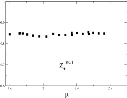
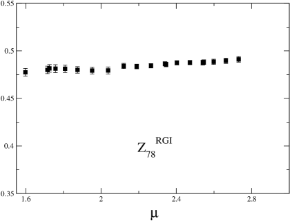
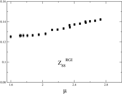
Figure 1: $Z^{RGI}$ defined in eq. (48), with $w_{+}$, $\hat{w}$ computed at NLO in perturbation theory and ${\cal Z}_{+}(\mu)$, $\hat{\cal Z}(\mu)$ computed non-perturbatively in the RI-MOM scheme. The scale $\mu$ is in GeV.

Although the computed values of the $Z^{RGI}$ in fig. 1 are independent of $\mu$ to a reasonable precision, we see that especially for ${\cal Z}_{88}$ the plateau is worse than in the other cases. This could be due either to lattice artefacts or to the possibility that higher order contributions to the RG evolution may be significant. The detailed study in ref. [54], using data from simulations at four values of the lattice spacing, suggests that the lattice artefacts are not large and interpret the deviation from scaling as being due to N²LO perturbative corrections. As emphasized in ref. [54] it would be desirable to control better the scaling behaviour by evaluating the N²LO anomalous dimensions and/or performing a step-scaling analysis.

We extract ${\cal Z}_{+}^{RGI}$ and $\hat{\cal Z}^{RGI}$ by fitting each of the plateaus in fig. 1 to a constant in the interval $2.1\mbox{ GeV}\leq\mu\leq 2.4\mbox{ GeV}$. We then use eq. (48) to obtain the value of the renormalization constants at the required scale. A standard scale at which the matrix elements are matched with the Wilson coefficients is $\mu=2\mbox{ GeV}$. At this value of $\mu$, the values of the renormalization constants in the RI-MOM scheme are

$${\cal Z}^{RI-MOM}_{+} = 0.601(3)\left({}^{+6}_{-9}\right)$$ (50)

$$\hat{{\cal Z}}^{RI-MOM} = \left(\begin{array}[]{cc}\phantom{-}0.664(2)\left({}^{+3}_{-8}\right)&-0.142(1)\left({}^{+2}_{-2}\right)\\ -0.055(1)\left({}^{+1}_{-2}\right)&\phantom{-}0.360(3)\left({}^{+21}_{-21}\right)\\ \end{array}\right)\,.$$ (53)

The first error is statistical while the second one is the systematic uncertainty estimated as explained in sec. 6.2. The conversion to the $\overline{\mbox{MS}}$-NDR and $\overline{\mbox{MS}}$-HV renormalization schemes can be readily done by using eqs. (31)-(38) (we take $\alpha^{\overline{\mbox{MS}}}_{s}(\mu=2\mbox{ GeV})=0.1953$ obtained in the quenched approximation at NLO with $\Lambda_{QCD}=0.250\mbox{ GeV}$). The non-perturbatively obtained results in eqs. (50) and (53) are remarkably similar to the perturbative results in eq. (42) (the similarity is less remarkable if mean field improvement is used to estimate the higher order terms in perturbation theory). Moreover, we can compare our non-perturbative results, computed with the data sets 1 and 2, with the ones obtained previously in ref. [54] at the same $\beta$ but using a smaller volume and data set 1 only. In this study, a complete basis of five parity odd $\Delta I=3/2$ operators was considered. For our purposes we only need to consider three of these, namely (in the notation of ref. [51]) ${\cal Q}^{+}_{1}$, ${\cal Q}^{+}_{2}$, and ${\cal Q}^{+}_{3}$. In fact, with the appropriate choice of flavour quantum numbers, there is the following correspondence between the two notations:

$${\cal O}_{4}\equiv 2{\cal Q}^{+}_{1},\ \ {\cal O}^{3/2}_{7}\equiv 2{\cal Q}^{+}_{2},\ \ {\cal O}^{3/2}_{8}\equiv-4{\cal Q}^{+}_{3};$$

$${\cal Z}_{+}\equiv{\cal Z}_{11},\ {\cal Z}_{77}\equiv{\cal Z}_{22},\ \ {\cal Z}_{78}\equiv-\frac{1}{2}\,{\cal Z}_{23},\ \ {\cal Z}_{88}\equiv{\cal Z}_{33},\ \ {\cal Z}_{87}\equiv-2\,{\cal Z}_{32},$$ (54)

and the renormalization structure is therefore the one indicated in eqs. (16) and (26). The values obtained in ref. [54] were the following,

$$\begin{array}[]{rccc}{\cal Z}^{RI-MOM}_{+}&=&0.608(4)(14)&0.604(3)(5)\\ \hat{{\cal Z}}^{RI-MOM}&=&\left(\begin{array}[]{cc}\phantom{-}0.673(3)(10)&-0.139(1)(5)\\ -0.056(2)(2)&\phantom{-}0.392(3)(28)\\ \end{array}\right)&\left(\begin{array}[]{cc}\phantom{-}0.666(3)(3)&-0.140(1)(2)\\ -0.056(2)(2)&\phantom{-}0.375(3)(14)\\ \end{array}\right)\\ \end{array}$$ (55)

where the first corresponds to the small volume $16^{3}\times 52$ and the second to data set 1. As can be seen by comparing eqs.(50) and (53) with eq.(55), the agreement is excellent, suggesting that finite-volume effects are very small.

5 The Analysis

In this section we discuss the analysis of our results, starting with the extraction of the matrix elements. We then discuss the determination of the shift of the energy of the two-pions as a result of finite-volume effects and finally we explain our procedure for the chiral extrapolation.

5.1 Extraction of the Matrix Elements

We now explain the procedure we use to determine the matrix elements in the SPQR kinematics [14, 15], where one of the final-state pions has a non-zero spatial momentum, and the other two mesons are at rest. In order to remove the $I=1$ component in the two-pion state, we take the symmetric combination of the two states $|\pi^{+}({\vec{p}}^{\,})\pi^{0}(\vec{0})\rangle$ and $|\pi^{+}(\vec{0})\pi^{0}(\vec{p}^{\,})\rangle$, where $|\vec{p\,}|=0$ or $2\pi/L$, i.e. we evaluate the following average:

$${\mathcal{M}}^{(i)}_{\mathrm{SPQR}}(M_{\pi},E_{\pi},M_{K})=\frac{1}{2}\left(\langle\pi^{+}(\vec{p}^{\,})\pi^{0}(\vec{0})|{\mathcal{O}}_{i}|K^{+}(\vec{0})\rangle+\langle\pi^{+}(\vec{0})\pi^{0}(\vec{p}^{\,})|{\mathcal{O}}_{i}|K^{+}(\vec{0})\rangle\right),$$ (56)

where $E_{\pi}$ is the energy of the corresponding pion and ${\mathcal{O}}_{i}$ are the operators defined in eqs. (1)-(3).

In Euclidean space, up to NLO precision in the chiral expansion and neglecting finite-volume effects, the magnitude of ${\mathcal{M}}^{(i)}_{\mathrm{SPQR}}$ can be extracted from the ratios of correlation functions

$$\frac{1}{2}\left(\frac{C^{(i)}_{+}(t,\vec{p}^{\,})+C^{(i)}_{0}(t,\vec{p}^{\,})}{C_{K}(t_{\textrm{\scriptsize{fix}}},\vec{0})C_{\pi}(t_{\textrm{\scriptsize{fix}}},\vec{0})C_{\pi}(t,\vec{p}^{\,})}\right)(a^{6}Z_{\pi}^{2}Z_{K})\stackrel{{\scriptstyle\mathrm{large}\mbox{ }t}}{{\longrightarrow}}a^{3}\bar{{\mathcal{M}}}^{(i)}_{\mathrm{SPQR}},$$ (57)

where $C^{(i)}_{+}$ and $C^{(i)}_{0}$ are defined in eq.(3) and $\bar{{\mathcal{M}}}^{(i)}_{\mathrm{SPQR}}$ represents the magnitude of the matrix element of the bare lattice operator $\bar{{\mathcal{O}}}_{i}$ on the right-hand side of eq. (56). $Z_{P}=\langle 0|\phi_{P}(0)|P\rangle$ is the wave-function renormalization of the pseudoscalar meson state $P$, and can be obtained from the fit to

$$C_{P}(t,\vec{0})=\frac{(a^{2}Z_{P})^{2}}{aM_{P}}\ {\mathrm{e}}^{-aM_{P}\frac{T}{2}}\ {\mathrm{cosh}}\left[aM_{P}\left(\frac{T}{2}-t\right)\right],$$ (58)

at large $t$, where $T$ is the number of time slices (T=64 in this study). Fig. 2 shows some of the plateaus for $a^{3}\bar{{\mathcal{M}}}^{(i)}_{\mathrm{SPQR}}$.

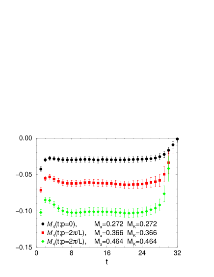
Figure 2: Plateaus for the extraction of the form factors $a^{3}\bar{{\mathcal{M}}}^{(i)}_{\mathrm{SPQR}}$.

The value of the pseudoscalar decay constant $f_{P}$ corresponding to the (non-degenerate) mass $M_{P}$ is obtained via the one-parameter fit (using $Z_{P}$ and $M_{P}$ obtained from eq. (58))

$$\left(\frac{C_{PA}(t,\vec{0})}{C_{PP}(t,\vec{0})}\right)\times\left(\frac{Z_{P}}{M_{P}}\right)=\left(\frac{f_{P}a}{Z_{A}}\right)\times{\mathrm{tanh}}\left[aM_{P}\left(\frac{T}{2}-t\right)\right],$$ (59)

at large $t$. In order to obtain $f$ we neglect the effects of $SU(3)$ breaking and we extrapolate quadratically on the smallest 5 masses. We obtain $f=0.139(5)\mbox{ GeV}$ from data set 1 and $f=0.135(4)\mbox{ GeV}$ from set 2. The renormalization constant $Z_{A}$ is determined non-perturbatively, as discussed in sec. 4.

Eq. (57) corresponds to the case in which NLO $\chi$PT is applicable and in which finite-volume effects are neglected. More generally we use the finite-volume formalism of refs. [25, 26] to write:

$$\frac{1}{2}\left(\frac{C^{(i)}_{+}(t,\vec{p})+C^{(i)}_{0}(t,\vec{p})}{C_{K}(t_{\textrm{\scriptsize{fix}}},\vec{0})C_{\pi}(t_{\textrm{\scriptsize{fix}}},\vec{0})C_{\pi}(t,\vec{p})}\right)(a^{3}Z_{\pi}^{2}Z_{K}) \stackrel{{\scriptstyle\mathrm{large}\mbox{ }t}}{{\longrightarrow}}$$ (60)

$$\left\{a^{3}|\bar{{\mathcal{M}}}^{(i)}_{\mathrm{SPQR}}|\cos\delta^{I=2}(W)+O\left(\frac{1}{L}\right)\right\}e^{-\Delta Wt_{\textrm{\scriptsize{fix}}}},$$

where $W$ is the two pion energy in a finite volume so that $\Delta W\equiv W-E_{\pi}-M_{\pi}$ and $\delta^{I=2}(W)$ is the $I=2$ two-pion phase shift. We now discuss the finite-volume effects in more detail.

5.2 Two Pion Energy Shift in a Finite Volume

In this section we discuss the extraction of the energy shift of the two-pion state with the SPQR kinematics, $\Delta W\equiv W-E_{\pi}-M_{\pi}$, using a data set of 750 configurations (of which set 1 is the subset on which the four-point functions were also computed). We consider pions of three masses, each composed of a degenerate quark-antiquark pair. The masses of the pions in lattice units are $M_{\pi}=$ 0.4438(7), 0.3590(8) and 0.2557(13) corresponding to hopping parameters $\kappa=0.13300,$ 0.13376 and 0.13449 respectively.

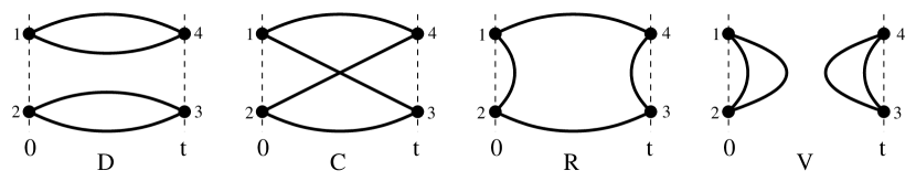
Figure 3: Feynman diagrams which appear in the computation of the most generic four pion correlation function as $G_{4\pi}(t,\vec{p\,})$ in the $SU(2)$ symmetric limit.

Consider the correlation function

$$G_{4\pi}(t,\vec{p\,}) = \frac{1}{2}\Big{(}\left\langle P_{\pi^{+}}(t,\vec{p\,})P_{\pi^{0}}(t,\vec{0}\,)\phi_{\pi^{+}}^{\dagger}(\vec{0}\,,0)\phi_{\pi^{0}}^{\dagger}(\vec{0}\,,0)\right\rangle$$ (61)

$$\hskip 21.68121pt+\left\langle P_{\pi^{+}}(t,\vec{0}\,)P_{\pi^{0}}(t,\vec{p\,})\phi_{\pi^{+}}^{\dagger}(\vec{0}\,,0)\phi_{\pi^{0}}^{\dagger}(\vec{0}\,,0)\right\rangle\Big{)}$$

where the interpolating operators in momentum and position space, $P_{\pi}$ and $\phi_{\pi}$ respectively, are defined in eq. (13). We have symmetrized over the two interpolating operators at fixed momentum $P_{\pi^{+}}$ and $P_{\pi^{0}}$ in order to obtain a pure $I=2$ state. The most general four-pion correlation function may be represented in terms of the four diagrams in fig. 3. Moreover, in the $SU(2)$ symmetric limit, since the two interpolating operators at $t=0$ are at the same spatial point, the symmetrization performed in eq. (61) is automatic. The $I=2$ correlation function in eq. (61) is given by the combination $D-C$ of diagrams in fig. 3, while the corresponding $I=0$ correlator is given by the combination $D+C/2-3R+3/2V$. Here we only consider the $I=2$ channel, which is the relevant one for $\Delta I=3/2\$transitions.

To determine the two-pion energy shift $\Delta W$, we compute the ratio

$$R_{4\pi}(t;\vec{p\,})\equiv\frac{G_{4\pi}(t;\vec{p\,})}{C_{\pi}(t,\vec{p\,})C_{\pi}(t,\vec{0}\,)}\,,\$$ (62)

where $C_{\pi}$ is defined in eq. (14), and, in order to isolate the lightest states, we consider the behaviour of the correlation functions in the region $T\gg t\gg 0$.

On a lattice with periodic boundary condition in the temporal direction $G_{4\pi}$ has two types of contribution; either a two-pion state propagates between 0 and $t$ (or between $t$ and $T$) or there is a single pion propagating between 0 and $t$ and another between $t$ and $T$. In the region $T\gg t\gg 0$ the ratio is therefore given by:

$$R_{4\pi}(t,\vec{p\,}) \longrightarrow \frac{X_{1}\big{(}e^{-Wt}+e^{-W(T-t)}\big{)}+X_{2}\big{(}e^{-E_{\pi}t}e^{-M_{\pi}(T-t)}+e^{-M_{\pi}t}e^{-E_{\pi}(T-t)}\big{)}}{X_{3}\big{(}e^{-M_{\pi}t}+e^{-M_{\pi}(T-t)}\big{)}\big{(}e^{-E_{\pi}t}+e^{-E_{\pi}(T-t)}\big{)}}$$ (63)

$$=\frac{X_{1}e^{-W\frac{T}{2}}\cosh\big{(}W(t-\frac{T}{2})\big{)}+X_{2}e^{-\frac{(M_{\pi}+E_{\pi})}{2}T}\cosh\big{(}(E_{\pi}-M_{\pi})(t-\frac{T}{2}))}{2\;X_{3}e^{-\frac{(M_{\pi}+E_{\pi})}{2}T}\cosh\big{(}M_{\pi}(t-\frac{T}{2})\big{)}\cosh\big{(}E_{\pi}(t-\frac{T}{2})\big{)}}$$

where the constants $X_{1,2,3}$ are independent of time but do depend on the finite volume energies of the $|\pi\rangle$ and $|\pi\pi\rangle$ states. $E_{\pi}$ is the energy of a pion with momentum $\vec{p\,}$. We have not displayed the contribution of the excited states.

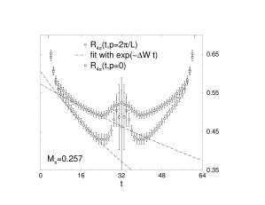
Figure 4: (a) $R_{4\pi}(t,\vec{p\,})$ for $aM_{\pi}=0.257$ and for both momenta, on the whole lattice. (b) $R_{4\pi}(t,\vec{p\,}_{\textrm{\scriptsize{min}}})$ for the three masses of the pion.

In fig. 4 (a) we plot $R_{4\pi}(t,\vec{0}\,)$ and $R_{4\pi}(t,\vec{p\,}_{\textrm{\scriptsize{min}}})$ as a function of $t$ for the lightest quark mass (corresponding to $\kappa=0.13449$). $|\vec{p\,}_{\textrm{\scriptsize{min}}}|=2\pi/L$ and we average over the six equivalent directions. In fig. 4 (b) we plot $R_{4\pi}(t,\vec{p\,}_{\textrm{\scriptsize{min}}})$ for all three pion masses. In order to determine $\Delta W$ we have to fit the $R_{4\pi}(t,\vec{p\,})$’s in a range of $t$ such that the first term in the numerator of eq. (63) dominates over the second. This condition is in addition to the usual requirement that the time intervals are sufficiently large for the contributions from excited states to be suppressed. In practice we extract the energy shifts by fitting $R_{4\pi}(t,\vec{p\,})$ to $A\exp(-\Delta Wt)$ in the range $t\in[14-15,\,22-23]$ (symmetrizing the contributions from the correlation functions over times in the forward and backward halves of the lattice), with the exact choice of interval depending on the mass and momentum. In order to estimate the systematic error, we vary the limits of the time interval used for the fit and look at the spread of the values thus obtained. The results are reported in tab. 2 (preliminary results were presented in ref. [32]).

$M_{\pi}$	0.4438(7)	0.3590(8)	0.2557(13)
$\Delta W_{\vec{p\,}=0}$	0.0054(6)(7)	0.0062(7)(7)	0.0066(9)(7)
$\Delta W_{\vec{p\,}=\frac{2\pi}{L}}$	0.0086(8)(10)	0.0109(11)(15)	0.0152(27)(15)
$\Delta W_{L}$	0.0064(3)	0.0072(3)	0.0083(5)
$\Delta W_{BG}$	0.0052(2)	0.0060(2)	0.0071(3)

Table 2: Numerical results ($\Delta W_{\vec{p\,}=0}$ and $\Delta W_{\vec{p\,}=\frac{2\pi}{L}}$) and theoretical predictions ($\Delta W_{L}$ and $\Delta W_{BG}$ for $\vec{p\,}=0$, defined in eqs. (64) and (67)). For the numerical results, which are given in lattice units, we quote statistical and systematic uncertainties in that order.

In tab. 2 we also present theoretical predictions for the energy shift obtained using the Lüscher formula and tree-level $\chi$PT in full QCD ($\Delta W_{L}$) [59, 60, 61, 62] and by using one-loop quenched $\chi$PT ($\Delta W_{BG}$) [30]. In both cases the predictions are for $\vec{p\,}=0$. In spite of reservations that our pion masses may be too large for $\chi$PT to be applicable, the agreement of our lattice results with the theoretical predictions from one-loop quenched $\chi$PT is very good and reassuring. On the other hand, we observe discrepancies between our results and the predictions of Luscher’s formula (which however is obtained in full QCD). We now outline the determination of $\Delta W_{L}$ and $\Delta W_{BG}$.

The Lüscher formula for the energy shift gives

$$\Delta W_{L}=W-2M_{\pi}=-\frac{4\pi a_{0}}{M_{\pi}L^{3}}\left\{1+c_{1}\frac{a_{0}}{L}+c_{2}\frac{a_{0}^{2}}{L^{2}}\right\}+O(L^{-6})\,,$$ (64)

$$\textrm{where}\qquad c_{1}=-2.837297,\qquad c_{2}=6.375183$$ (65)

and $a_{0}$ is the scattering length in the $s$-wave, $I=2$ channel. At tree level in full $\chi$PT

$$a_{0}=-\frac{M_{\pi}}{8\pi f_{\pi}^{2}}\;.$$ (66)

We use the values of $M_{\pi}$ obtained in our simulation and the corresponding values of $f_{\pi}(M_{\pi})$.

$\Delta W_{BG}$ is obtained by using one-loop quenched ChPT:

$$\Delta W_{BG}=\Delta W^{\textrm{\scriptsize{tree}}}+\Delta W^{\textrm{\scriptsize{1-loop}}}=\frac{1}{2f_{\pi}^{2}L^{3}}+M_{\pi}\left(B_{2}(M_{\pi}L)\delta^{2}+A_{2}(M_{\pi}L)\delta\epsilon+O\Big{(}\frac{\epsilon^{2}}{(M_{\pi}L)^{3}}\Big{)}\right)$$ (67)

where the first term corresponds to the leading term in the Lüscher formula after substitution of the expression for the scattering length in eq. (66), while the second term comes from one-loop diagrams. In the region of large $M_{\pi}L$, $A_{2}(M_{\pi}L)$ and $B_{2}(M_{\pi}L)$ can be approximated by

$$A_{2}(M_{\pi}L)\simeq\frac{1}{\pi}\left(\frac{2\pi}{M_{\pi}L}\right)^{3}\qquad\textrm{and}\qquad B_{2}(M_{\pi}L)\simeq-\frac{1}{6\pi}\left(\frac{2\pi}{M_{\pi}L}\right)^{3}\;.$$ (68)

Finally

$$\delta\equiv\frac{m_{0}^{2}/3}{8\pi^{2}f_{\pi}^{2}}\qquad\textrm{and}\qquad\epsilon\equiv\frac{M_{\pi}^{2}}{16\pi^{2}f_{\pi}^{2}}\,,$$ (69)

where $m_{0}$ is the $\eta^{\prime}$ mass. Taking the full QCD estimate $m_{0}^{2}/3=(500\mbox{ MeV})^{2}$ would give $\delta\sim 0.18$. We vary $\delta$ between $0.08$ and $0.18$ (which is approximately the range of values typically obtained in quenched simulations). In this interval, however, the one-loop contribution is small for the parameters of our simulation, and we observe a very mild dependence of $\Delta W_{BG}$ on $\delta$ which is included in the quoted uncertainty. In tab. 2 we present the results obtained for $\delta=0.10$.

In our data set 2 for $K\to\pi\pi$ decays we have not evaluated the correlation function $G_{4\pi}$ and therefore cannot determine $\Delta W$ at the corresponding pion masses directly. However, as shown in tab. 1 the pion masses in this data set are very close to those in set 1 and we therefore obtain the energy shifts at these masses by interpolating or extrapolating the results obtained in set 1. We find that for the pion masses $aM_{\pi}=$ 0.4642, 0.3663 and 0.2716, the corresponding $a\Delta W_{\vec{p\,}=0}=$ 0.0052, 0.0061, 0.0065 and $a\Delta W_{\vec{p\,}=\frac{2\pi}{L}}=$ 0.0080, 0.0107, 0.0146.

Finally we use the extracted values of $\Delta W_{\vec{p\,}}$ for SPQR kinematics to correct the ratio on the left-hand side of eq. (60) for the finite-volume effects $e^{-\Delta Wt_{\textrm{\scriptsize{fix}}}}$. Results for the matrix elements of bare operators obtained in this way with $\cos(\delta)=1$ are reported in tab. 3. They still contain finite-volume effects, and in order to remove these one would need to know the Lellouch-Lüscher factors for SPQR kinematics. These are currently unknown and we estimate the corresponding errors in sec. 6.3.

$\#$	$\bar{\mathcal{M}}^{(4)}_{\rm SPQR}(\vec{0}\,)$	$\bar{\mathcal{M}}^{(4)}_{\rm SPQR}(\vec{p\,}_{\textrm{\scriptsize{min}}})$	$\bar{\mathcal{M}}^{(7)}_{\rm SPQR}(\vec{0}\,)$	$\bar{\mathcal{M}}^{(7)}_{\rm SPQR}(\vec{p\,}_{\textrm{\scriptsize{min}}})$	$\bar{\mathcal{M}}^{(8)}_{\rm SPQR}(\vec{0}\,)$	$\bar{\mathcal{M}}^{(8)}_{\rm SPQR}(\vec{p\,}_{\textrm{\scriptsize{min}}})$
Set 1 (340 configurations)
1a	0.0236(40)	0.0294(50)	0.199(20)	0.159(17)	0.695(71)	0.613(64)
2a	0.0298(42)	0.0384(68)	0.199(21)	0.157(15)	0.704(71)	0.620(65)
3a	0.0354(48)	0.0454(77)	0.202(22)	0.157(15)	0.725(72)	0.631(63)
1b	0.0521(55)	0.0570(66)	0.194(16)	0.167(14)	0.747(60)	0.685(56)
2b	0.0604(61)	0.0657(70)	0.195(15)	0.167(13)	0.767(59)	0.698(56)
3b	0.0712(73)	0.0769(82)	0.191(15)	0.162(13)	0.777(59)	0.702(56)
1c	0.0846(79)	0.0864(84)	0.191(14)	0.167(13)	0.815(61)	0.754(57)
2c	0.0952(87)	0.0972(92)	0.191(14)	0.167(12)	0.834(60)	0.771(58)
3c	0.1020(94)	0.1044(99)	0.187(14)	0.164(12)	0.834(60)	0.770(59)
Set 2 (480 configurations)
1a	0.0297(38)	0.0398(57)	0.187(14)	0.163(11)	0.687(47)	0.647(40)
2a	0.0320(37)	0.0428(57)	0.188(12)	0.166(11)	0.701(45)	0.661(39)
3a	0.0347(37)	0.0457(56)	0.190(12)	0.167(10)	0.713(44)	0.669(37)
4a	0.0374(39)	0.0487(56)	0.192(11)	0.170(10)	0.723(43)	0.679(36)
5a	0.0397(40)	0.0513(56)	0.193(11)	0.171(10)	0.729(42)	0.685(35)
6a	0.0416(42)	0.0538(57)	0.193(11)	0.172(10)	0.732(42)	0.691(35)
7a	0.0449(44)	0.0576(59)	0.194(11)	0.174(10)	0.740(42)	0.697(35)
1b	0.0583(43)	0.0636(50)	0.190(12)	0.170(10)	0.770(41)	0.718(35)
2b	0.0557(43)	0.0610(51)	0.190(11)	0.167(10)	0.761(42)	0.703(34)
3b	0.0615(44)	0.0671(50)	0.190(11)	0.171(10)	0.777(40)	0.730(35)
4b	0.0654(46)	0.0713(51)	0.192(10)	0.173(10)	0.789(39)	0.746(34)
5b	0.0681(47)	0.0743(51)	0.192(10)	0.174(10)	0.795(39)	0.751(34)
6b	0.0707(47)	0.0771(52)	0.192(10)	0.174(10)	0.800(38)	0.756(35)
1c	0.1012(54)	0.1025(57)	0.195(11)	0.176(10)	0.884(40)	0.833(37)
2c	0.0944(53)	0.0949(57)	0.194(12)	0.174(10)	0.868(42)	0.807(37)
3c	0.0973(53)	0.0982(57)	0.194(11)	0.175(10)	0.874(41)	0.819(37)
4c	0.1059(55)	0.1077(58)	0.195(10)	0.178(10)	0.896(39)	0.847(37)
5c	0.1088(55)	0.1107(57)	0.196(10)	0.179(10)	0.902(38)	0.855(37)

Table 3: Numerical values of the bare amplitudes $\bar{{\mathcal{M}}}^{(4,7,8)}_{\rm SPQR}(\vec{p\,})\equiv\bar{{\mathcal{M}}}^{(4,7,8)}_{\rm SPQR}(M_{\pi},E_{\pi}(\vec{p\,}),M_{K})$ as obtained from the ratio on the l.h.s. of eq. (60) multiplied by the FV correction $e^{\Delta Wt_{\textrm{\scriptsize{fix}}}}$. $M_{\pi}$ assumes the values 1a, 1b, 1c and $M_{K}$ respectively $\{1a,2a,\ldots\}$, $\{1b,2b,\ldots\}$, $\{1c,2c,\ldots\}$.

5.3 Chiral Extrapolations and the Numerical Results

We start by fitting our lattice data to the formulae of the NLO chiral expansion, including the chiral logarithms obtained in ref. [15], determine the low energy constants and use these to extrapolate to the physical point. When applicable, we use the numerical values for the couplings $\alpha=0.1$ and $m_{0}=0.5\mbox{ GeV}$ in the terms $\alpha(\partial_{\mu}\Phi_{0})(\partial^{\mu}\Phi_{0})-m^{2}_{0}\Phi^{2}_{0}$ of the quenched chiral Lagrangian, where $\Phi_{0}$ is the super-$\eta^{\prime}$ field. The results are not very sensitive to the variation of $\alpha$ and $m_{0}$ within a reasonable range. The fits are poor, which may not be surprising since we are trying to use the chiral expansion in a range of masses and energies which are rather large ($[0.52,1.5]\mbox{ GeV}$). To improve the situation we have also performed fits in restricted intervals, introducing an upper cut-off for the masses and energies (we vary this cut-off down to a value of 0.8 GeV). Since the validity of quenched $\chi$PT (q$\chi$PT) may be questioned even in the restricted interval we have also performed fits using only the polynomial terms of q$\chi$PT (i.e. the NLO expressions from q$\chi$PT but without the logarithms) which have the same functional form as those in $\chi$PT of full QCD.

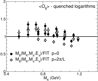
Figure 5: Plots illustrating the relative quality of the q$\chi$PT and polynomial fits for $\langle{\mathcal{O}}_{8}\rangle$. The 18 points for each of the two values of momentum correspond to the masses from data set 2 in tab. 1 and are plotted as a function of $M_{K}$.

Of the fits which we have tried the best results have been obtained using the polynomial fits. This is illustrated in fig. 5, where we display the ratio of the lattice amplitude and the fitted amplitude for q$\chi$PT and polynomial fits. This exercise shows that the NLO polynomial correction are essential to describe the data in the range we have simulated, whereas the addition of the chiral logarithms (which have fixed coefficients) spoils the quality of the fits. Since at sufficiently low masses the NLO chiral logarithms must be present, we have also tried the centaur procedure in which we smoothly match the polynomial fits (the horse) to the NLO $\chi$PT formula (the man) at some kinematical point. The details of the matching procedure will be described below. The centaur procedure allows us to estimate the systematic uncertainty in the extrapolation of our data to the physical point. Of course, these uncertainties will not be fully under control until simulations in full QCD are performed at sufficiently small masses so that the NLO $\chi$PT formula is seen to hold.

We perform the fits on the two subsets of our data corresponding to the two independent simulations:

1. in set 1 masses and energies have values in the interval $[0.52,1.5]\mbox{ GeV}$;

2. in set 2 their values are restricted to be in the interval $[0.54,1.2]\mbox{ GeV}$. This set was generated in order to increase the number of points at smaller masses.

We start with a discussion of the evaluation of ${}_{I=2}\langle\pi\pi|{\mathcal{O}}_{7,8}|K^{0}\rangle$ for which we need only a relatively small number of low energy constants (five, one at LO and four more at NLO). In addition the chiral expansion starts at $O(M_{\pi,K}^{0})$ (rather then $O(M_{\pi,K}^{2})$) and so the fits are much more stable and an estimate of the matrix elements is possible to a reasonable accuracy. As explained above, in addition to using NLO q$\chi$PT formulae, we also fit the data to the polynomial obtained by removing the chiral logarithms.

The results obtained using the procedures described above are presented in tab. 4. $\langle{\mathcal{O}}_{7,8}\rangle_{I=2}^{\textrm{\scriptsize{phys}}}$ represents the value of the matrix element at physical values of the masses, energies and momenta at NLO in the chiral expansion. By $\langle{\mathcal{O}}_{7,8}\rangle_{I=2}^{\gamma}$ we denote the contribution of the leading order to the physical result. Note that this is the value of the matrix element in the chiral limit, which is the quantity determined from previous studies, in which only $K\rightarrow\pi$ matrix elements were calculated. We observe from tab. 4 (see also fig. 5) that the polynomial form gives by far the best description of our lattice data for ${}_{I=2}\langle\pi\pi|{\mathcal{O}}_{7,8}|K^{0}\rangle$, indicating that the data are not in the kinematic range where the NLO chiral expansion for these amplitudes are valid.

From our study we see that the use of q$\chi$PT does not describe our lattice data and therefore using fits based on q$\chi$PT alone can lead to unreasonable results. However, in a more general context, it has been argued that one may combine the behaviour expected in chiral perturbation theory at low masses with the observed polynomial dependence on the kinematical parameters in lattice simulations  [63, 64]. We now attempt to perform such a matching.

fit ansatz	points	$\langle{\mathcal{O}}_{7}\rangle_{I=2}^{\textrm{\scriptsize{phys}}}$	$\langle{\mathcal{O}}_{7}\rangle_{I=2}^{\gamma}$	$\frac{\chi}{d.o.f}$	$\langle{\mathcal{O}}_{8}\rangle_{I=2}^{\textrm{\scriptsize{phys}}}$	$\langle{\mathcal{O}}_{8}\rangle_{I=2}^{\gamma}$	$\frac{\chi}{\textrm{d.o.f}}$
Set 1 (340 configurations)
poly., $M_{K},E_{\pi}<1.5$	18	0.130(15)	0.155(16)	0.11	0.746(91)	0.802(99)	0.024
poly., $M_{K},E_{\pi}<1.2$	13	0.135(15)	0.161(17)	0.13	0.750(93)	0.792(98)	0.020
poly., $M_{K},E_{\pi}<1.0$	10	0.140(16)	0.161(17)	0.10	0.753(93)	0.790(98)	0.015
q$\chi$PT, $M_{K},E_{\pi}<1.5$	18	0.203(21)	0.308(32)	14.8	1.37(17)	2.06(27)	8.95
q$\chi$PT, $M_{K},E_{\pi}<1.2$	13	0.302(32)	0.492(51)	5.83	1.51(19)	2.32(30)	3.46
q$\chi$PT, $M_{K},E_{\pi}<1.0$	10	0.276(29)	0.477(50)	4.86	1.37(18)	2.20(29)	2.88
Set 2 (480 configurations)
poly., $M_{K},E_{\pi}<1.2$	36	0.127(11)	0.143(12)	0.022	0.734(64)	0.761(70)	0.022
poly., $M_{K},E_{\pi}<1.0$	24	0.128(12)	0.143(13)	0.014	0.732(68)	0.754(74)	0.019
poly., $M_{K},E_{\pi}<0.8$	16	0.132(13)	0.142(13)	0.013	0.732(77)	0.753(77)	0.025
q$\chi$PT, $M_{K},E_{\pi}<1.2$	36	0.268(26)	0.425(42)	13.4	1.53(16)	2.33(26)	11.0
q$\chi$PT, $M_{K},E_{\pi}<1.0$	24	0.265(28)	0.442(47)	7.71	1.47(16)	2.34(27)	6.36
q$\chi$PT, $M_{K},E_{\pi}<0.8$	16	0.224(25)	0.412(47)	6.06	1.22(14)	2.18(26)	5.01

Table 4: Results obtained using various fitting procedures to our data for the matrix elements ${}_{I=2}\langle\pi\pi|{\mathcal{O}}_{7}|K^{0}\rangle$ and ${}_{I=2}\langle\pi\pi|{\mathcal{O}}_{8}|K^{0}\rangle$ renormalised in the NDR-$\overline{\mbox{MS}}$ scheme at $2\mbox{ GeV}$. Energies and masses are given in GeV while the matrix elements are in $\mbox{ GeV}^{3}$. When fitting using the q$\chi$PT formula we take $\alpha=0.1$ and $m_{0}=0.5\mbox{ GeV}$. Notice that we perform uncorrelated fits, which is the reason for the very small $\chi^{2}/$d.o.f. for good fits.

For the most general kinematics the amplitudes ${\mathcal{M}}^{(7,8)}$ are function of the Lorentz invariants $p_{\pi^{+}}^{2}=p_{\pi^{0}}^{2}=M_{\pi}^{2}$, $p_{K}^{2}=M_{K}^{2}$, $p_{K}\cdot p_{\pi^{+}}$, $p_{K}\cdot p_{\pi^{0}}$ and $p_{\pi^{+}}\cdot p_{\pi^{0}}$, where $p_{K}$, $p_{\pi^{+}}$ and $p_{\pi^{0}}$ are four-momenta of the kaon and the two pions. The $I=2$ $|\pi^{+}\pi^{0}\rangle$ final state is symmetric and therefore the dependence on $p_{K}\cdot p_{\pi^{+}}$ and on $p_{K}\cdot p_{\pi^{0}}$ is the same. In the region of small masses and energies the matrix element is given by $\chi$PT at NLO, which for ${\mathcal{O}}_{8}$, for example, takes the form:

$${\mathcal{M}}^{(8),\chi{\mathrm{PT}}}_{\mathrm{general}} = A_{(\chi)}\left(1+[{\mathrm{chiral}}\mbox{ }{\mathrm{log}}]_{\mathrm{gen}}(M^{2}_{K},M^{2}_{\pi},p_{\pi^{+}}\cdot p_{K},p_{\pi^{0}}\cdot p_{K},p_{\pi^{+}}\cdot p_{\pi^{0}})\right)$$ (70)

$$+B_{1(\chi)}M^{2}_{K}+B_{2(\chi)}(p_{\pi^{+}}+p_{\pi^{0}})\cdot p_{K}+B_{3(\chi)}M^{2}_{\pi}+B_{4(\chi)}(p_{\pi^{+}}\cdot p_{\pi^{0}}),$$

where $A_{(\chi)}$ and the $B_{i(\chi)}$’s are unknown constants. On the other hand, in the region accessible to our simulation the data are well described by a polynomial of the form:

$$\!\!\!\!\!\!\!{\mathcal{M}}^{(8),\mathrm{poly}}_{\mathrm{general}} = A_{(p)}+B_{1(p)}M^{2}_{K}+B_{2(p)}(p_{\pi^{+}}+p_{\pi^{0}})\cdot p_{K}+B_{3(p)}M^{2}_{\pi}+B_{4(p)}(p_{\pi^{+}}\cdot p_{\pi^{0}})\,.$$ (71)

Our procedure is to fit the lattice data to eq. (71), extract $A_{(p)}$ and the $B_{i(p)}$’s and then to impose the following smoothness condition

$$\left({\mathcal{M}}^{(8),\chi{\mathrm{PT}}}_{\mathrm{general}}\right)_{\mathrm{SPQR\ m.p.}} = \left({\mathcal{M}}^{(8),\mathrm{poly}}_{\mathrm{general}}\right)_{\mathrm{SPQR\ m.p.}},$$

$$\left(\frac{\partial{{\mathcal{M}}^{(8),\chi{\mathrm{PT}}}_{\mathrm{general}}}}{\partial\,\omega_{i}}\right)_{\mathrm{SPQR\ m.p.}} = \left(\frac{\partial{{\mathcal{M}}^{(8),\mathrm{poly}}_{\mathrm{general}}}}{\partial\,\omega_{i}}\right)_{\mathrm{SPQR\ m.p.}},$$ (72)

where the $\omega_{i},\ i=1$ – 4, are the four variables $M^{2}_{K},M^{2}_{\pi},p_{\pi^{+}}\cdot p_{\pi^{0}}$ and $p_{K}\cdot p_{\pi^{+}}$. The subscript “SPQR m.p.” indicates that the matching point is chosen in the SPQR kinematics and is thus defined by the values of the masses of the pion and kaon and the energy of the moving pion ($M_{\pi}^{\ast},M_{K}^{\ast},E_{\pi}^{\ast}$) at which the matching is performed. This set of conditions determines the values of $A_{(\chi)}$ and $B_{i(\chi)}$, which can then be used to compute the physical amplitude using

$${\mathcal{M}}^{(8),\chi{\mathrm{PT}}}_{\mathrm{phys}} = A_{(\chi)}\left(1+[{\mathrm{chiral}}\mbox{ }{\mathrm{log}}]_{\mathrm{phys}}(m^{2}_{K},m^{2}_{\pi})\right)$$ (73)

$$+\left(B_{1(\chi)}+B_{2(\chi)}+\frac{1}{2}B_{4(\chi)}\right)m_{K}^{2}+\left(B_{3(\chi)}-B_{4(\chi)}\right)m_{\pi}^{2}.$$

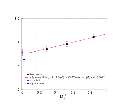
Figure 6: $\chi$PT-polynomial matching for $\langle{\mathcal{O}}_{8}\rangle_{I=2}$ (in GeV³) at $(M_{\pi}^{\ast},E_{\pi}^{\ast},M_{K}^{\ast})=(0.4,0.4,0.41)\mbox{ GeV}$ (we plot only data points with $M_{\pi}=E_{\pi}=M_{K}$). For reasons of numerical stability, it is convenient to use a matching point in which $M_{K}^{\ast}$ is offset from $M_{\pi}^{\ast}$ and $M_{\pi}^{\ast}$. The point labelled as chiral limit corresponds to $M_{\pi}=E_{\pi}=M_{K}=0$ and that labelled as physical point corresponds to the physical values of the masses and energies, and hence does not lie on the SPQR curve.

Tab. 5 shows the results for ${}_{I=2}\langle\pi\pi|{\mathcal{O}}_{7,8}|K^{0}\rangle$ from this centaur procedure, with different choices of matching points. An example of this procedure is represented graphically in fig. 6.

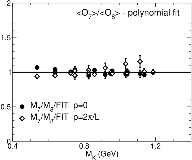
Figure 7: Quality of the polynomial fit for $\langle{\mathcal{O}}_{7}\rangle/\langle{\mathcal{O}}_{8}\rangle$.

In the ratio ${\cal M}^{(7)}/{\cal M}^{(8)}$ chiral logarithms and finite-volume corrections cancel since the two operators belong to the same representation [65]. This ratio can also be used to compare lattice results to other theoretical approaches [66, 67, 68, 69, 70]. Results are reported in tab. 6. In contrast to the case of $\langle{\mathcal{O}}_{7}\rangle$ and $\langle{\mathcal{O}}_{8}\rangle$ individually, this ratio is not so well described by the polynomial form coming from $\chi$PT. This is clear by comparing the values for the $\chi^{2}/$d.o.f of tab. 6 with those of tab. 4 and also by comparing fig. 7 with fig. 5. We will discuss these results in sec. 7.

Implicit in our work is the assumption that, in the region in which we have data, the lattice results are reliable even though the simulations have been performed in the quenched approximation. When performing the centaur matching we join the polynomial fit of our data with the NLO $\chi$PT formula corresponding to full QCD. At low masses and energies (where we do not have data) the behaviour predicted by quenched $\chi$PT is very different from that in full QCD. However, in spite of the fact that we have data from a quenched simulation it does not make sense to extrapolate to the physical point using q$\chi$PT. Our central value for ${}_{I=2}\langle\pi\pi|{\mathcal{O}}_{7,8}|K^{0}\rangle$ is obtained by the centaur matching, with full chiral logarithms, at the matching point $(M_{\pi}^{*},E_{\pi}^{*},M_{K}^{*})=(0.4,0.4,0.5)\mbox{ GeV}$. At the same time we also obtain the estimate of the LECs in full QCD reported in tab. 7. Other results reported in these tables are used to estimate systematic errors, and will be discussed in detail in sec. 6.1.

$M_{\pi}^{*}$	$M_{K}^{*}$	$\langle{\mathcal{O}}_{7}\rangle_{I=2}^{\textrm{\scriptsize{phys}}}$	$\langle{\mathcal{O}}_{7}\rangle_{I=2}^{\gamma}$	$\langle{\mathcal{O}}_{8}\rangle_{I=2}^{\textrm{\scriptsize{phys}}}$	$\langle{\mathcal{O}}_{8}\rangle_{I=2}^{\gamma}$	$\frac{\langle{\mathcal{O}}_{7}\rangle_{I=2}^{\textrm{\scriptsize{phys}}}}{\langle{\mathcal{O}}_{8}\rangle_{I=2}^{\textrm{\scriptsize{phys}}}}$
poly. fit		$0.130(15)\left({}^{+8}_{-13}\right)$	$0.155(16)\left({}^{+8}_{-14}\right)$	$0.746(91)\left({}^{+49}_{-59}\right)$	$0.802(99)\left({}^{+53}_{-64}\right)$	0.174
poly. fit		$0.127(11)\left({}^{+7}_{-8}\right)$	$0.143(12)\left({}^{+8}_{-8}\right)$	$0.734(64)\left({}^{+44}_{-44}\right)$	$0.761(70)\left({}^{+46}_{-46}\right)$	0.173
matching in the SPQR kinematics ($E_{\pi}^{*}=M_{\pi}^{*}$) with full logarithms
0.3	0.5	$0.127(14)\left({}^{+8}_{-13}\right)$	$0.154(16)\left({}^{+8}_{-14}\right)$	$0.728(89)\left({}^{+48}_{-58}\right)$	$0.799(99)\left({}^{+53}_{-64}\right)$	0.174
0.3	0.4	$0.123(14)\left({}^{+7}_{-12}\right)$	$0.159(17)\left({}^{+9}_{-15}\right)$	$0.708(86)\left({}^{+47}_{-56}\right)$	$0.821(101)\left({}^{+54}_{-66}\right)$	0.174
0.4	0.5	$0.119(14)\left({}^{+7}_{-12}\right)$	$0.163(17)\left({}^{+9}_{-15}\right)$	$0.691(84)\left({}^{+46}_{-55}\right)$	$0.843(104)\left({}^{+56}_{-67}\right)$	0.173
0.3	0.31	$0.114(13)\left({}^{+7}_{-12}\right)$	$0.160(17)\left({}^{+9}_{-15}\right)$	$0.663(81)\left({}^{+44}_{-53}\right)$	$0.829(102)\left({}^{+55}_{-66}\right)$	0.172
0.4	0.41	$0.113(13)\left({}^{+7}_{-12}\right)$	$0.164(17)\left({}^{+9}_{-15}\right)$	$0.656(80)\left({}^{+43}_{-52}\right)$	$0.851(105)\left({}^{+56}_{-68}\right)$	0.172
0.5	0.51	$0.113(13)\left({}^{+7}_{-12}\right)$	$0.170(18)\left({}^{+9}_{-16}\right)$	$0.660(80)\left({}^{+44}_{-53}\right)$	$0.882(109)\left({}^{+58}_{-71}\right)$	0.171
0.3	0.5	$0.124(11)\left({}^{+7}_{-7}\right)$	$0.143(12)\left({}^{+8}_{-8}\right)$	$0.716(62)\left({}^{+43}_{-43}\right)$	$0.758(70)\left({}^{+45}_{-46}\right)$	0.173
0.3	0.4	$0.121(11)\left({}^{+7}_{-7}\right)$	$0.147(12)\left({}^{+8}_{-8}\right)$	$0.698(60)\left({}^{+42}_{-42}\right)$	$0.779(72)\left({}^{+47}_{-47}\right)$	0.173
0.4	0.5	$0.117(11)\left({}^{+7}_{-7}\right)$	$0.151(13)\left({}^{+8}_{-8}\right)$	$0.682(59)\left({}^{+41}_{-41}\right)$	$0.800(74)\left({}^{+48}_{-48}\right)$	0.172
0.3	0.31	$0.112(10)\left({}^{+7}_{-7}\right)$	$0.148(12)\left({}^{+8}_{-8}\right)$	$0.655(56)\left({}^{+39}_{-39}\right)$	$0.786(73)\left({}^{+47}_{-47}\right)$	0.171
0.4	0.41	$0.111(10)\left({}^{+6}_{-7}\right)$	$0.152(13)\left({}^{+8}_{-8}\right)$	$0.648(56)\left({}^{+39}_{-39}\right)$	$0.807(75)\left({}^{+48}_{-49}\right)$	0.171
0.5	0.51	$0.112(10)\left({}^{+7}_{-7}\right)$	$0.158(13)\left({}^{+9}_{-9}\right)$	$0.652(56)\left({}^{+39}_{-39}\right)$	$0.836(77)\left({}^{+50}_{-50}\right)$	0.172
matching in the SPQR kinematics ($E_{\pi}^{*}=M_{\pi}^{*}$) with quenched logarithms
0.3	0.5	$0.135(15)\left({}^{+8}_{-14}\right)$	$0.184(19)\left({}^{+10}_{-17}\right)$	$0.772(94)\left({}^{+51}_{-62}\right)$	$0.953(117)\left({}^{+63}_{-76}\right)$	0.175
0.3	0.4	$0.133(15)\left({}^{+8}_{-13}\right)$	$0.180(19)\left({}^{+10}_{-17}\right)$	$0.763(93)\left({}^{+51}_{-61}\right)$	$0.936(115)\left({}^{+62}_{-75}\right)$	0.174
0.4	0.5	$0.139(16)\left({}^{+8}_{-14}\right)$	$0.208(22)\left({}^{+11}_{-19}\right)$	$0.794(97)\left({}^{+53}_{-63}\right)$	$1.07(13)\left({}^{+7}_{-9}\right)$	0.175
0.3	0.31	$0.130(15)\left({}^{+8}_{-13}\right)$	$0.178(19)\left({}^{+10}_{-16}\right)$	$0.743(91)\left({}^{+49}_{-59}\right)$	$0.923(114)\left({}^{+61}_{-74}\right)$	0.175
0.4	0.41	$0.135(15)\left({}^{+8}_{-14}\right)$	$0.203(21)\left({}^{+11}_{-19}\right)$	$0.771(94)\left({}^{+51}_{-61}\right)$	$1.05(13)\left({}^{+69}_{-84}\right)$	0.175
0.5	0.51	$0.153(17)\left({}^{+9}_{-15}\right)$	$0.246(26)\left({}^{+13}_{-23}\right)$	$0.866(106)\left({}^{+57}_{-69}\right)$	$1.27(16)\left({}^{+84}_{-102}\right)$	0.176
0.3	0.5	$0.132(12)\left({}^{+8}_{-8}\right)$	$0.170(14)\left({}^{+9}_{-9}\right)$	$0.758(66)\left({}^{+45}_{-46}\right)$	$0.905(84)\left({}^{+54}_{-55}\right)$	0.174
0.3	0.4	$0.130(12)\left({}^{+8}_{-8}\right)$	$0.167(14)\left({}^{+9}_{-9}\right)$	$0.750(65)\left({}^{+45}_{-45}\right)$	$0.888(82)\left({}^{+53}_{-54}\right)$	0.173
0.4	0.5	$0.136(12)\left({}^{+8}_{-8}\right)$	$0.192(16)\left({}^{+10}_{-11}\right)$	$0.779(68)\left({}^{+47}_{-47}\right)$	$1.02(9)\left({}^{+6}_{-6}\right)$	0.175
0.3	0.31	$0.127(11)\left({}^{+7}_{-7}\right)$	$0.165(14)\left({}^{+9}_{-9}\right)$	$0.731(63)\left({}^{+44}_{-44}\right)$	$0.876(81)\left({}^{+53}_{-53}\right)$	0.174
0.4	0.41	$0.132(12)\left({}^{+8}_{-8}\right)$	$0.188(16)\left({}^{+10}_{-10}\right)$	$0.757(66)\left({}^{+45}_{-46}\right)$	$0.995(92)\left({}^{+60}_{-60}\right)$	0.174
0.5	0.51	$0.149(13)\left({}^{+9}_{-9}\right)$	$0.227(19)\left({}^{+12}_{-13}\right)$	$0.848(74)\left({}^{+51}_{-51}\right)$	$1.21(11)\left({}^{+72}_{-73}\right)$	0.176

Table 5: Results for ${}_{I=2}\langle\pi\pi|{\mathcal{O}}_{7,8}|K^{0}\rangle$ via $\chi$PT-polynomial matching performed with full and quenched chiral logarithms from Set 1 (340 configurations), first block of results, and Set 2 (480 configurations), second block. The matrix elements are renormalised in the NDR-$\overline{\mbox{MS}}$ scheme at $2\mbox{ GeV}$. Energies and masses are in GeV while the matrix elements are in $\mbox{ GeV}^{3}$. In the q$\chi$PT formula we use $\alpha=0.1$ and $m_{0}=0.5\mbox{ GeV}$.

data sets	points	$\langle{\mathcal{O}}_{7}\rangle_{I=2}^{\textrm{\scriptsize{phys}}}/\langle{\mathcal{O}}_{8}\rangle_{I=2}^{\textrm{\scriptsize{phys}}}$	$\frac{\chi}{d.o.f}$
Set 1, $M_{K},E_{\pi}<1.5$	18	$0.157(12)\left({}^{+2}_{-5}\right)$	3.11
Set 1, $M_{K},E_{\pi}<1.0$	10	$0.171(11)\left({}^{+2}_{-3}\right)$	3.02
Set 2, $M_{K},E_{\pi}<1.2$	36	$0.153(10)\left({}^{+3}_{-2}\right)$	1.33
Set 2, $M_{K},E_{\pi}<0.8$	16	$0.163(10)\left({}^{+2}_{-2}\right)$	1.14

Table 6: Results of the polynomial fit for the ratio ${\cal M}^{(7)}/{\cal M}^{(8)}$ where the operators are renormalised in the NDR-$\overline{\mbox{MS}}$ scheme at $2\mbox{ GeV}$.

LECs	Set 1 ${\mathcal{O}}_{7}$	Set 2 ${\mathcal{O}}_{7}$	Set 1 ${\mathcal{O}}_{8}$	Set 2 ${\mathcal{O}}_{8}$
$\gamma/f^{3}[\rm{GeV}^{3}]$	0.0705(75)	0.0653(54)	0.365(45)	0.347(32)
$(4\pi f)^{2}(\delta_{1}+\delta_{2})/\gamma$	-0.42(90)	-1.08(59)	-1.20(64)	-1.64(53)
$(4\pi f)^{2}(\frac{\delta_{2}}{2}-\frac{\delta_{1}}{2}+\delta_{3})/\gamma$	-0.46(33)	-0.36(31)	-1.27(20)	-1.35(19)
$(4\pi f)^{2}(\delta_{4}+\delta_{5})^{\prime}/\gamma$	0.12(43)	-0.06(24)	0.66(26)	0.44(21)
$(4\pi f)^{2}\delta_{6}^{\prime}/\gamma$	-0.59(18)	-0.39(13)	-0.92(13)	-0.75(11)

Table 7: Results for the LECs of ${}_{I=2}\langle\pi\pi|{\mathcal{O}}_{7,8}|K^{0}\rangle$ (where operators are renormalised in the NDR-$\overline{\mbox{MS}}$ scheme at $2\mbox{ GeV}$) from the centaur matching with $(M_{\pi}^{*},E_{\pi}^{*},M_{K}^{*})=(0.4,0.4,0.5)\mbox{ GeV}$. Only statistical errors are displaied. The values for $f$ are $0.139(5)\mbox{ GeV}$ from set 1 and $0.135(4)\mbox{ GeV}$ from set 2. For the definitions of $(\delta_{4}+\delta_{5})^{\prime}$ and $\delta_{6}^{\prime}$ see eq. (2).

We now turn to the matrix elements of the operator ${\mathcal{O}}_{4}$. There is one LEC at leading order in $\chi$PT and six more at NLO, so that the fits to the NLO chiral expansion have seven parameters. Again we find that our data is not well represented by quenched chiral perturbation theory at NLO. If instead we remove the chiral logarithms from the fit, we do obtain fits with reasonable values of $\chi^{2}$. The coefficients of the polynomial terms at NLO (which would correspond to the NLO LECs if the chiral logarithms had been included) are very poorly determined however, making any extrapolation to the chiral limit impossible. On the other hand, the coefficient of the leading term is found to be stable, and is significantly lower (by about 40%) than the value obtained keeping only LO chiral perturbation theory. Thus the contribution of the NLO terms is clearly visible even if, due to the high number of free parameters in the fit, it is not possible to evaluate the corresponding LECs with sufficient precision. We therefore do not discuss further the evaluation of the matrix elements of ${\mathcal{O}}_{4}$ beyond showing one indicative plot. In fig. 8 we plot the values of the bare matrix element $\bar{\cal M}^{(4)}_{\rm SPQR}(\vec{0})$ from dataset 2 at the three values of the pion mass with degenerate quarks. Also shown are linear and quadratic fits to these three points, from which it can be seen that the extrapolated value in the chiral limit is close to zero as expected from chiral perturbation theory (indeed the quadratic fit gives a value consistent with zero). However, until we have lattice data in the chiral regime, plots such as that in fig. 8 are at best qualitative.

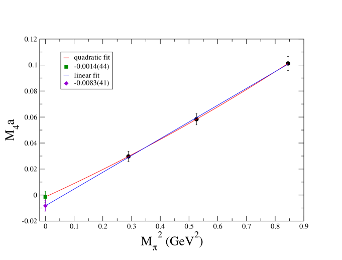
Figure 8: Chiral behaviour of the bare amplitude (in lattice units) $\bar{\cal M}^{(4)}_{\rm SPQR}(\vec{0})$ for pions with degenerate quarks (lines 1a, 1b, 1c of Tab.3 for dataset 2) versus $M_{\pi}^{2}$. The numbers in the box correspond to the extrapolated values in the chiral limit.

6 Systematic uncertainties

We now discuss the main systematic errors which affect the values for the renormalized matrix elements of the electroweak penguins obtained in this work.

6.1 Uncertainties from the chiral extrapolation

Our results indicate that we are not in a regime where q$\chi$PT is valid. Completely reliable results can only be obtained by performing full QCD simulations in a regime where $\chi$PT describes the data and can therefore be used for the extrapolation to the physical point. In the meantime we use the centaur procedure of matching the polynomials which describe our data to the NLO chiral expansion for $\langle\pi^{+}\pi^{0}|\bar{{\mathcal{O}}}^{3/2}_{7,8}|K^{+}\rangle$. This procedure is valid under the assumption that there is an overlap region in which both descriptions hold. We estimate the corresponding systematic error by varying the matching point below our data down to the chiral limit (the results are insensitive to varying the cut-off on the masses and energies of our data points).

6.2 Uncertainties from operator matching

The main source of systematic error in the evaluation of the renormalization constants is the residual dependence on the renormalization scale $\mu$ of ${\cal Z}_{+}^{RGI}$ and $\hat{\cal Z}^{RGI}$ in eq. (48). As explained in sec. 4.3, this residual dependence is probably due to higher order corrections not taken into account by the NLO perturbative evaluation of the evolution functions $w_{+}$ and $\hat{w}$. Since the scale $\mu=2\mbox{ GeV}$ at which we evaluate the renormalization constants lies inside the range of momenta at which we compute the renormalization constants, we estimate the systematic error in the following way: we take the renormalization constants computed non-perturbatively at a given scale $\mu_{0}$ and we run them up or down to the required scale $\mu$. The systematic error is then estimated from the deviations of the results obtained by varying $\mu_{0}$ in the whole range in which we compute numerically the renormalization constants (i.e. $\mu_{0}\in[1.6,2.75]\mbox{ GeV}$). In order to reduce this uncertainty we would need to perform simulations at larger values of $a^{-1}$.

6.3 Uncertainties from the $\pi{-}\pi$ phase shift and the finite-volume effects

In this study we have used matrix elements computed with the SPQR kinematics for which the two-pion system is not at rest. The Lellouch-Lüscher (LL) factor relating the finite-volume matrix elements to physical amplitudes is valid in the centre-of-mass frame, and the corresponding formula for the moving frame is currently unknown. This introduces a systematic error and underlines the importance of developing a theory of finite-volume effects for two-meson states in a moving frame. Using the LL factor as a guide with phase-shifts estimated using $\chi$PT we expect these corrections to be of order 10-15%, but their effect on the chiral extrapolation is difficult to estimate.

As shown in sec. 5.1 and 5.2, we were able to eliminate the systematic error coming from the shift $\Delta W$ of the two-pion energy in a finite volume. After applying this correction, since we divide the correlator $C^{(i)}_{+}+C^{(i)}_{0}$ by two non-interacting pion propagators (see eq. (57)), we obtain the matrix element multiplied by the cosine of the phase-shift, $\cos(\delta^{I=2}(W))$. For the data points in which both pions are at rest, $\delta^{I=2}(W)=0$ and there is no correction. For those where one of the two pions has non zero momentum (i.e. in a moving frame), a first attempt to study the relation between the finite-volume energy shift and the infinite volume phase-shift has been presented in ref. [71] but a thorough understanding of this problem proves to be very involved and might not be resolved soon. For this reason we give here only an approximate estimate of $\cos(\delta^{I=2}(W))$ based on the computation of the phase shifts obtained with $N_{f}=2$ dynamical simulations in the laboratory frame [72]. For all of the pion masses in our simulation $\cos(\delta^{I=2}(W))$ turns out to be larger than $0.98$.

6.4 Quenching effects

A reliable estimation of the quenching effects can only be obtained when the unquenched (or partially quenched) lattice data are available. The matrix elements presented in this paper have dimension three, therefore suffer from the uncertainties in the determination of the lattice spacing, which is one effect of the quenched approximation. By performing phenomenological studies using ratios of matrix elements it may be hoped that the uncertainty is reduced, but it must be remembered that quenching errors remain and that simulations with dynamical quarks will be required to eliminate them.

7 Final results

Our final results from the two data sets (at the precision of NLO in the chiral expansion) are

$${}_{I=2}\langle\pi\pi|{\mathcal{O}}_{8}|K^{0}\rangle^{\textrm{\scriptsize{NLO}}}_{\textrm{\scriptsize{phys}}} = 0.691(84)\left({}^{+46}_{-55}\right)\left({}^{+55}_{-35}\right)\mbox{ GeV}^{3}$$

$${}_{I=2}\langle\pi\pi|{\mathcal{O}}_{7}|K^{0}\rangle^{\textrm{\scriptsize{NLO}}}_{\textrm{\scriptsize{phys}}} = 0.119(14)\left({}^{+7}_{-12}\right)\left({}^{+11}_{-6}\right)\mbox{ GeV}^{3}$$ (74)

from set 1 and

$${}_{I=2}\langle\pi\pi|{\mathcal{O}}_{8}|K^{0}\rangle^{\textrm{\scriptsize{NLO}}}_{\textrm{\scriptsize{phys}}} = 0.682(59)\left({}^{+41}_{-41}\right)\left({}^{+52}_{-34}\right)\mbox{ GeV}^{3}$$

$${}_{I=2}\langle\pi\pi|{\mathcal{O}}_{7}|K^{0}\rangle^{\textrm{\scriptsize{NLO}}}_{\textrm{\scriptsize{{phys}}}} = 0.117(11)\left({}^{+7}_{-7}\right)\left({}^{+10}_{-6}\right)\mbox{ GeV}^{3}$$ (75)

from set 2, where the matrix elements are renormalized in the NDR-$\overline{\mbox{MS}}$ scheme at $2\mbox{ GeV}$ . The first error is statistical, the second is due to the uncertainties in the non-perturbative matching to the continuum renormalization scheme and the third is due to the $\chi$PT-polynomial matching. In estimating the third error, we have taken the central value as that obtained by matching to full chiral logarithms at $(M_{\pi}^{\ast},M_{K}^{\ast})=$ (0.4 GeV, 0.5 GeV), the lower limit to be the value obtained by matching at (0.4 GeV, 0.41 GeV) and the upper limit to be the value obtained from the polynomial fit. With this choice, the error bar spans the range of values in the top half of table 5. The results from the two data sets are consistent and as our best estimate we take

$${}_{I=2}\langle\pi\pi|{\mathcal{O}}_{8}|K^{0}\rangle^{\textrm{\scriptsize{NLO}}}_{\textrm{\scriptsize{phys}}} = 0.68\,(6)\,(4)\,(5)\mbox{ GeV}^{3}$$

$${}_{I=2}\langle\pi\pi|{\mathcal{O}}_{7}|K^{0}\rangle^{\textrm{\scriptsize{NLO}}}_{\textrm{\scriptsize{phys}}} = 0.12\,(1)\,(1)\,(1)\mbox{ GeV}^{3}\,.$$ (76)

Taking the ratio of these two matrix elements directly at the physical point we obtain the values

$$\frac{{}_{I=2}\langle\pi\pi|{\mathcal{O}}_{7}|K^{0}\rangle^{\textrm{\scriptsize{NLO}}}_{\textrm{\scriptsize{phys}}}}{{}_{I=2}\langle\pi\pi|{\mathcal{O}}_{8}|K^{0}\rangle^{\textrm{\scriptsize{NLO}}}_{\textrm{\scriptsize{phys}}}} = 0.173(17)\left({}^{+2}_{-4}\right)\left({}^{+1}_{-2}\right)\qquad\textrm{from set 1}$$

$$\frac{{}_{I=2}\langle\pi\pi|{\mathcal{O}}_{7}|K^{0}\rangle^{\textrm{\scriptsize{NLO}}}_{\textrm{\scriptsize{phys}}}}{{}_{I=2}\langle\pi\pi|{\mathcal{O}}_{8}|K^{0}\rangle^{\textrm{\scriptsize{NLO}}}_{\textrm{\scriptsize{phys}}}} = 0.172(14)\left({}^{+2}_{-2}\right)\left({}^{+1}_{-1}\right)\qquad\textrm{from set 2}\,.$$ (77)

The last error is again due to the uncertainty in the $\chi$PT-polynomial matching. From the last column of tab. 5 one can appreciate how this ratio is independent of the effects of the chiral logarithms, i.e. from the choice of the matching point $(M_{\pi}^{*},E_{\pi}^{*},M_{K}^{*})$ and from the use of $\chi$PT or q$\chi$PT formulae. The results in eq. (77) can be compared with those obtained from the polynomial fit of the ratio ${\cal M}^{(7)}/{\cal M}^{(8)}$ in tab. 6 (which has a relatively poor $\chi^{2}$). By reducing the range of masses and energies used in the fit, its quality increases and the values for the ratio get closer to those reported in eq. (77).

The contribution of the leading order term to the matrix elements, which also corresponds to their value in the chiral limit, is

$${}_{I=2}\langle\pi\pi|{\mathcal{O}}_{8}|K^{0}\rangle_{\gamma} = 0.843(104)\left({}^{+56}_{-67}\right)\left({}^{+40}_{-45}\right)\mbox{ GeV}^{3}$$

$${}_{I=2}\langle\pi\pi|{\mathcal{O}}_{7}|K^{0}\rangle_{\gamma} = 0.163(17)\left({}^{+9}_{-15}\right)\left({}^{+7}_{-9}\right)\mbox{ GeV}^{3}$$ (78)

from set 1 and

$${}_{I=2}\langle\pi\pi|{\mathcal{O}}_{8}|K^{0}\rangle_{\gamma} = 0.800(74)\left({}^{+48}_{-48}\right)\left({}^{+35}_{-40}\right)\mbox{ GeV}^{3}$$

$${}_{I=2}\langle\pi\pi|{\mathcal{O}}_{7}|K^{0}\rangle_{\gamma} = 0.151(13)\left({}^{+8}_{-8}\right)\left({}^{+7}_{-8}\right)\mbox{ GeV}^{3}$$ (79)

from set 2, where the sources of errors are the same as in eq. (74). From eqs. (74) and (78), it is clear that the NLO contribution of the chiral expansion is significant. It tends to decrease these matrix elements by about $15-25\%$. In the kinematical range of the lattice data these NLO contributions are very significant. In fact, had we computed the matrix elements at LO in $\chi$PT (i.e. by fitting our data points to a constant) we would have obtained the following results:

$${}_{I=2}\langle\pi\pi|{\mathcal{O}}_{8}|K^{0}\rangle^{\textrm{\scriptsize{LO}}}_{\textrm{\scriptsize{phys}}} = 0.951(74)\mbox{ GeV}^{3}$$

$${}_{I=2}\langle\pi\pi|{\mathcal{O}}_{7}|K^{0}\rangle^{\textrm{\scriptsize{LO}}}_{\textrm{\scriptsize{phys}}} = 0.082(9)\mbox{ GeV}^{3}$$ (80)

from set 1 and

$${}_{I=2}\langle\pi\pi|{\mathcal{O}}_{8}|K^{0}\rangle^{\textrm{\scriptsize{LO}}}_{\textrm{\scriptsize{phys}}} = 0.979(45)\mbox{ GeV}^{3}$$

$${}_{I=2}\langle\pi\pi|{\mathcal{O}}_{7}|K^{0}\rangle^{\textrm{\scriptsize{LO}}}_{\textrm{\scriptsize{phys}}} = 0.082(9)\mbox{ GeV}^{3}$$ (81)

from set 2.

	$\langle{\mathcal{O}}_{7}\rangle_{I=2}^{\gamma}$ [GeV3]	$\langle{\mathcal{O}}_{8}\rangle_{I=2}^{\gamma}$ [GeV3]	$\langle{\mathcal{O}}_{7}\rangle_{I=2}^{\gamma}/\langle{\mathcal{O}}_{8}\rangle_{I=2}^{\gamma}$
This work	$0.16(3)$	$0.82(15)$	0.19(3)
Donini et al. [74]	$0.11(4)$	$0.51(10)$	0.22(9)
RBC [10]	$0.27(3)$	$1.1(2)$	0.25(5)
CP-PACS [11]	$0.24(3)$	$1.0(2)$	0.24(6)
Friot et al. [70]	$0.12(2)$	$2.00(36)$	0.057(15)
Cirigliano et al. [68]	$0.16(10)$	$2.22(67)$	0.07(5)
Bijnens et al. [67]	$0.24(3)$	$1.2(8)$	0.20(14)
Cirigliano et al. [69]	$0.22(5)$	$1.50(27)$	0.15(4)
Narison [66]	$0.21(5)$	$1.40(35)$	0.15(5)

Table 8: Numerical results for the matrix elements of ${\mathcal{O}}_{7}$ and ${\mathcal{O}}_{8}$ (renormalised in the NDR-$\overline{\mbox{MS}}$ scheme at $2\mbox{ GeV}$) in the chiral limit from various methods (lattice, dispersion relations, large $N_{c}$+MHA, sum rules).

In tab. 8 we compare our results with those obtained using different methods (including lattice simulations, dispersion relations, large $N_{c}$+MHA and QCD sum rules). None of the lattice estimates includes the quenching error. The three previous lattice computations [74, 10, 11] used $K\rightarrow\pi$ matrix elements and $\chi$PT at leading order to obtain $K\to\pi\pi$ amplitudes in the chiral limit. The present work is the first computation with two pions in the final state which allows the use of $\chi$PT at NLO to extrapolate to the physical point and to the chiral limit. All of the lattice computations have been performed at fixed value of the lattice spacing, but with different actions, different methods of computing the renormalization factors and different method of performing the chiral extrapolation, making it very difficult to compare the systematic uncertainties and to understand the source of the discrepancy among different results. In the next generation of computations it will be important to perform simulations at several values of the lattice spacing in order to study the approach to the continuum limit, as well as going to lighter values of the quark masses (the relatively high-values of masses used in current and previous simulations is one of the major limitations).

The range of values for $\langle{\mathcal{O}}_{8}\rangle_{I=2}^{\gamma}$ obtained using lattice simulations is lower than that obtained using other techniques (although they do overlap within errors). For $\langle{\mathcal{O}}_{7}\rangle_{I=2}^{\gamma}$ there are discrepancies between the different lattice simulations and similar discrepancies using other techniques. Finally, one of the main conclusions of the present study is that the NLO contribution of $\chi$PT at the physical point decreases the value of the matrix elements by a $15-25\%$. This is a physical effect which will affect all the estimates presented in tab. 8.

8 Conclusions

It can be argued that $K\to\pi\pi$ decay amplitudes represent the Holy Grail of lattice simulations, since so many theoretical and technical difficulties must be overcome before they can be calculated reliably. The aim of this study was to get a better understanding of the practicability of computing correlation functions with two-pion final states. This is necessary for extending calculations beyond leading order in chiral perturbation theory. Specifically in this paper we have presented the first attempt to calculate the matrix elements for $K\to\pi\pi$ decays with an $I=2$ final state and to determine all the low energy constants which appear at next-to-leading order in the chiral expansion. We were able to carry out all the necessary steps but with varying degrees of precision and success. Our best estimates for the matrix elements of the electroweak penguin operators are presented in sec. 7 (see, for example, eq. (76)). In addition to the quoted errors should be added those due to the use of the quenched approximation and finite-volume corrections. Although we could also determine the matrix elements of the operator ${\cal O}_{4}$ at the masses which we used in the simulation, we were unable to determine the seven low-energy constants with sufficient precision to perform the chiral extrapolation. For all three operators we conclude that the NLO terms are significant.

The positive aspects of our exploratory study include:

1. For the $I=2$ channel, the finite-volume energy shift can be determined from the linear behaviour of the ratio $R_{4\pi}$ defined in eq. (62).

2. The $K\to\pi\pi$ matrix elements can be determined with good precision at the values of the masses used in the simulation.

3. The non-perturbative renormalization of the operators can be performed successfully.

In addition to removing the quenched approximation by performing simulations with dynamical quarks, we conclude that two major improvements are needed before reliable and precise results can be obtained using the techniques of this paper:

1. Simulations have to be performed in a region of light-quark masses where $\chi$PT is valid at NLO for $K\to\pi\pi$ matrix elements and which is sufficiently large that the low energy constants can be determined precisely enough for the extrapolation to the physical point to be possible. We have seen that this is not the case for the masses used in this simulation and for this reason we had to use the centaur procedure for the chiral extrapolation. This needs to be eliminated.

2. A theory of finite-volume corrections needs to be developed for two-pion states with a non-zero (total) momentum. For the spectrum this issue was studied in ref. [71]. For alternative procedures to determine the low-energy constants at next-to-leading order, which exploit more the freedom to vary the quark masses in lattice simulations rather than introducing a non-zero momentum for the $\pi\pi$ system see ref. [75].

Some minor improvements to our study can be made relatively easily. For example, the factor of $\cos(\delta)$ due to the two-pion sink (and the corresponding finite-volume effects) can be eliminated by computing four-pion correlation functions. This would also provide a consistency check on the value of the finite-volume energy shift.

Acknowledgements

We thank Damir Becirevic, Jonathan Flynn, Massimo Testa and Giovanni Villadoro for useful discussions, and Federico Rapuano for his participation in this work at the early stage. We are grateful to Alessandro Lonardo, Davide Rossetti and Piero Vicini for their constant technical support concerning the APEmille machines. C.-J.D.L. thanks Universitá di Roma “La Sapienza”, and M.P. thanks the University of Southampton for hospitality during the progress of this project. CJDL, GM, MP and CTS thank Maarten Golterman and Santi Peris for hospitality during the Benasque workshop on Matching Light Quarks to Hadrons where this work was completed.

This work was supported by DOE (USA) grants DE-FG02-00ER41132, DE-FG03-97ER41014 and DE-FG03-96ER40956, European Union grant HTRN-CT-2000-00145, MCyT Plan Nacional I+D+I (Spain) under Grant BFM2002-00568, and PPARC (UK) grants PPA/G/S/1998/00529 and PPA/G/O/2002/00468.

Appendix A Mass Dependence of $K\to\pi$ Matrix Elements.

In this appendix we consider the chiral behaviour of a simpler quantity than the $K\to\pi\pi$ matrix elements described in the body of the paper, viz. the $K\to\pi$ matrix elements from the quenched simulation of ref. [11]. For illustration we consider the matrix element of the operator ${\mathcal{O}}^{3/2}_{8}$ and show that the uncertainties due to the extrapolation in the quark mass are also significant in this case.

In figs. 9 and 10, we present the results obtained using different ansätze for the chiral fits to the quenched data for the ratio $\langle\pi^{+}|{\mathcal{O}}^{3/2}_{8}|K^{+}\rangle f_{\pi}/f_{M}^{2}$ (taken from ref.[11]). The matrix element $\langle\pi^{+}|{\mathcal{O}}^{3/2}_{8}|K^{+}\rangle$ is determined for $M_{K}=M_{\pi}\equiv M_{M}$. $f_{\pi}\approx 132$ MeV is the physical pion decay constant, and $f_{M}$ is the decay constant of the pseudoscalar meson with the mass $M_{M}$. In order to estimate the physical result we perform the following procedures:

1. We fit the lattice data to a quadratic function of the form $A^{(p)}_{0}+A^{(p)}_{2}M^{2}_{M}+A^{(p)}_{4}M^{4}_{M}$. The fit is shown in figs 9 and 10.

2. We also fit the data to the prediction of $\chi$PT of the form $A^{(\chi)}_{0}(1+[{\mathrm{chiral}}\mbox{ }{\mathrm{log}}])+A^{(\chi)}_{2}M^{2}_{M}$. The chiral logarithms in full QCD for $\langle\pi^{+}|{\mathcal{O}}^{3/2}_{8}|K^{+}\rangle$ can be obtained from ref. [76]. In the quenched theory, the corresponding chiral logarithms have been calculated in ref. [77]. These fits in full and quenched QCD are also shown in figs. 9 and 10 respectively.

3. Finally we carry out the centaur procedure of matching the polynomial fits to the lattice data (which again are good representations of the data) to chiral perturbation theory at lower masses. In the same way as for the $K\to\pi\pi$ matrix elements discussed in sec. 5, we assume that there is a region where both the polynomial and $\chi$PT behaviour are valid so that by matching the two forms at some scale (which, in figs. 9 and 10 is chosen to be 465 MeV) we can obtain the coefficients $A^{(\chi)}_{i}$ of the chiral expansion from the fitted coefficients $A^{(p)}_{i}$. We perform the matching by equating the value of $\langle\pi^{+}|{\mathcal{O}}^{(3/2)}_{8}|K^{+}\rangle f_{\pi}/f_{M}^{2}$ and its first derivative with respect to $M^{2}_{M}$ at the matching scale.

These figures show that the choice of the ansatz for performing chiral extrapolation can indeed result in large systematic errors, because the lattice simulation is carried out at relatively heavy quark masses. See for example fig. 9, where the matrix element in the chiral limit using the polynomial fit and extrapolation is about twice that obtained with the centaur procedure.

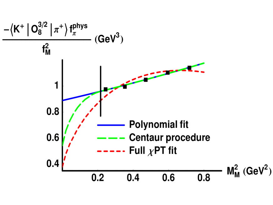
Figure 9: $K\to\pi$ matrix element using data from ref. [11]. The $\chi$PT fit corresponds to full QCD. The vertical line indicates the value of $M_{M}=465$ MeV where the $\chi$PT-polynomial matching is performed.

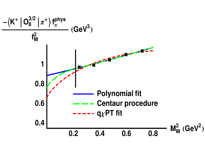
Figure 10: $K\to\pi$ matrix element using data from ref. [11]. The $\chi$PT fit corresponds to quenched QCD. The vertical line indicates the value of $M_{M}=465$ MeV where the $\chi$PT-polynomial matching is performed.

References

- [1] J. R. Batley et al., Phys. Lett. B544, 97 (2002).
- [2] A. Alavi-Harati et al., Phys. Rev. D67, 012005 (2003).
- [3] M. B. Gavela et al., Nucl. Phys. B306, 677 (1988).
- [4] C. W. Bernard and A. Soni, Nucl. Phys. Proc. Suppl. 9, 155 (1989).
- [5] C. W. Bernard and A. Soni, Nucl. Phys. Proc. Suppl. 17, 495 (1990).
- [6] C. Bernard, in From Actions to Answers, edited by T. DeGrand and D. Toussaint (World Scientific, Singapore, 1990).
- [7] R. Gupta, T. Bhattacharya, and S. Sharpe, Phys. Rev. D 55, 4036 (1997).
- [8] L. Conti et. al., Phys. Lett. B 421, 273 (1998).
- [9] L. Lellouch and C.-J. D. Lin, Nucl. Phys. Proc. Suppl. 73, 312 (1999).
- [10] T. Blum et al., Phys. Rev. D68, 114506 (2003).
- [11] J. I. Noaki et al., Phys. Rev. D68, 014501 (2003).
- [12] C. Bernard et al., Phys. Rev. D 32, 2343 (1985).
- [13] S. Aoki et. al. (JLQCD Collaboration), Phys. Rev. D 58, 054503 (1998).
- [14] P. Boucaud et al., Nucl. Phys. Proc. Suppl. 106, 329 (2002).
- [15] C.-J. D. Lin et al., Nucl. Phys. B650, 301 (2003).
- [16] M. A. Shifman, A. I. Vainshtein, and V. I. Zakharov, Nucl. Phys. B120, 316 (1977).
- [17] J. Donoghue, E. Golowich, and B. Holstein, Phys. Lett. B 119, 412 (1982).
- [18] J. Bijnens and M. Wise, Phys. Lett. B 137, 245 (1984).
- [19] J. Flynn and L. Randall, Phys. Lett. B 224, 221 (1989), erratum: ibid. B 334, 580 (1990).
- [20] S. Bosch et al., Nucl. Phys. B565, 3 (2000).
- [21] M. Ciuchini et al., Phys. Lett. B573, 201 (2000).
- [22] S. Bertolini, J. O. Eeg, and M. Fabbrichesi, Phys. Rev. D63, 056009 (2001).
- [23] E. Pallante, A. Pich, and I. Scimemi, Nucl. Phys. B617, 441 (2001).
- [24] A. J. Buras and M. Jamin, JHEP 0401, 048 (2004).
- [25] L. Lellouch and M. Luscher, Commun. Math. Phys. 219, 31 (2001).
- [26] C.-J. D. Lin, G. Martinelli, C. T. Sachrajda, and M. Testa, Nucl. Phys. B619, 467 (2001).
- [27] C.-H. Kim and N.H. Christ, Nucl. Phys. B (Proc. Suppl.) 119, 365 (2003).
- [28] G. M. de Divitiis and N. Tantalo, hep-lat/0409154.
- [29] C.-J. D. Lin et al., Phys. Lett. B553, 229 (2003).
- [30] C. W. Bernard and M. F. L. Golterman, Phys. Rev. D53, 476 (1996).
- [31] C. J. D. Lin et al., Phys. Lett. B581, 207 (2004).
- [32] P. Boucaud et al., Nucl. Phys. Proc. Suppl. 106, 323 (2002).
- [33] D. Becirevic et al., Nucl. Phys. Proc. Suppl. 119, 359 (2003).
- [34] J. Gasser and H. Leutwyler, Nucl. Phys. B250, 465 (1985).
- [35] M. F. L. Golterman and K. C. Leung, Phys. Rev. D56, 2950 (1997).
- [36] B. Sheikholeslami and R. Wohlert, Nucl. Phys. B 259, 572 (1985).
- [37] M. Lüscher, S. Sint, R. Sommer, P. Weisz and U. Wolff, Nucl. Phys. B 491, 435 (1997).
- [38] G. Martinelli, Phys. Lett. B 141, 395 (1984).
- [39] C. Bernard, A. Soni and T. Draper, Phys. Rev. D 36, 3224 (1987).
- [40] C. Bernard, T. Draper, G. Hockney, and A. Soni, Nucl. Phys. (Proc. Suppl.) 4, 483 (1988).
- [41] A.J. Buras, M. Jamin, M.E Lautenbacher and P.H. Weisz, Nucl. Phys. B 370, 69 (1992), addendum: ibid. B 375, 501 (1992).
- [42] A. Buras, M. Jamin, M. Lautenbacher, and P. Weisz, Nucl. Phys. B 400, 37 (1993).
- [43] A. Buras, M. Jamin, and M. Lautenbacher, Nucl. Phys. B 400, 75 (1993).
- [44] A.J. Buras, M. Jamin, and M.E. Lautenbacher, Nucl. Phys. B 408, 209 (1993).
- [45] M. Ciuchini, E. Franco, G. Martinelli, and L. Reina, Nucl. Phys. B 415, 403 (1994).
- [46] M. Ciuchini et al., Z. Phys. C68, 239 (1995).
- [47] M. Ciuchini et al., Nucl. Phys. B523, 501 (1998).
- [48] G. Parisi, in High Energy Physics-1980, proceedings of the XX International Conference on High Energy Physics, L. Durand and L. G. Pondrom, editors, American Institute of Physics (1981), Madison, Wisconsin.
- [49] G. Lepage and P. Mackenzie, Phys. Rev. D 48, 2250 (1993).
- [50] G. Martinelli and C. Pittori and C. Sachrajda and M. Testa and A. Vladikas, Nucl. Phys. B 445, 81 (1995).
- [51] A. Donini et al., Eur. Phys. J. C10, 121 (1999).
- [52] E. Gabrielli, G. Martinelli, C. Pittori, G. Heatlie and C.T. Sachrajda, Nucl. Phys. B 362, 475 (1991).
- [53] M. Göckeler et. al., Nucl. Phys. B (Proc. Suppl.) 53, 896 (1997).
- [54] D. Becirevic et al., JHEP 08, 022 (2004).
- [55] J.-R. Cudell, A. Le Yaouanc and C. Pittori, Phys. Lett. B 454, 105 (1999).
- [56] S. Aoki et al., Phys. Rev. Lett. 82, 4392 (1999).
- [57] C. Dawson, Nucl. Phys. B (Proc. Suppl.) 94, 613 (2001).
- [58] L. Giusti and A. Vladikas, Phys. Lett. B 488, 303 (2000).
- [59] M. Lüscher, Commun. Math. Phys. 104, 177 (1986).
- [60] M. Lüscher, Commun. Math. Phys. 105, 153 (1986).
- [61] M. Lüscher, Nucl. Phys. B 354, 531 (1991).
- [62] M. Lüscher, Nucl. Phys. B 364, 237 (1991).
- [63] A. S. Kronfeld and S. M. Ryan, Phys. Lett. B543, 59 (2002).
- [64] D. Becirevic, S. Fajfer, S. Prelovsek, and J. Zupan, Phys. Lett. B563, 150 (2003).
- [65] D. Becirevic and G. Villadoro, Remarks on the hadronic matrix elements relevant to the SUSY mixing amplitudes, 2004, hep-lat/0408029.
- [66] S. Narison, Nucl. Phys. B593, 3 (2001).
- [67] J. Bijnens, E. Gamiz, and J. Prades, JHEP 10, 009 (2001).
- [68] V. Cirigliano, J. F. Donoghue, E. Golowich, and K. Maltman, Phys. Lett. B522, 245 (2001).
- [69] V. Cirigliano, J. F. Donoghue, E. Golowich, and K. Maltman, Phys. Lett. B555, 71 (2003).
- [70] S. Friot, D. Greynat, and E. de Rafael, JHEP 0410, 043 (2004).
- [71] K. Rummukainen and S. Gottlieb, Nucl. Phys. B450, 397 (1995).
- [72] T. Yamazaki et al., I = 2 pi pi scattering phase shift with two flavors of O(a) improved dynamical quarks, 2004, hep-lat/0402025.
- [73] S. Aoki et al., Phys. Rev. D67, 014502 (2003).
- [74] A. Donini, V. Gimenez, L. Giusti, and G. Martinelli, Phys. Lett. B470, 233 (1999).
- [75] J. Laiho and A. Soni, hep-lat/0306035.
- [76] V. Cirigliano and E. Golowich, Phys. Lett. B475, 351 (2000).
- [77] G. Villadoro, (private communication).