${\cal N}$=1 super Yang–Mills on a (3+1) dimensional transverse lattice with one exact supersymmetry

Motomichi Harada and Stephen Pinsky

Department of Physics
Ohio State University
Columbus OH 43210

We formulate ${\cal N}$=1 super Yang-Mills theory in 3+1 dimensions on a two dimensional transverse lattice using supersymmetric discrete light cone quantization in the large-$N_{c}$ limit. This formulation is free of fermion species doubling. We are able to preserve one supersymmetry. We find a rich, non-trivial behavior of the mass spectrum as a function of the coupling $g\sqrt{N_{c}}$, and see some sort of “transition” in the structure of a bound state as we go from the weak coupling to the strong coupling. Using a toy model we give an interpretation of the rich behavior of the mass spectrum. We present the mass spectrum as a function of the winding number for those states whose color flux winds all the way around in one of the transverse directions. We use two fits to the mass spectrum and the one that has a string theory justification appears preferable. For those states whose color flux is localized we present an extrapolated value for $m^{2}$ for some low energy bound states in the limit where the numerical resolution goes to infinity.

1 Introduction

In the past years, there has been a tremendous amount of progress in the analytical understanding of supersymmetric theories due to the discovery of AdS/CFT correspondence [1], using “orbifolding” [2], “orientifolding” [3, 4], or others. Recently Armoni, Shifman and Veneziano have shown that in the large $N_{c}$ limit a non-supersymmetric gauge theory with a Dirac fermion in the antisymmetric tensor representation is equivalent, both perturbatively and nonperturbatively, to ${\cal N}$=1 super Yang-Mills (SYM) theory in its bosonic sector [3]. Since for $N_{c}=3$ the non-supersymmetric gauge theory is just one-flavor QCD, even though we have to keep in mind $1/N_{c}$ corrections, knowing the nonperturbative properties of ${\cal N}$=1 SYM is of great importance from phenomenological viewpoint as well. Accordingly, one cannot stress enough the importance of being able to perform some nonperturbative numerical calculations for ${\cal N}$=1 SYM to test the predictions made by Armoni, Shifman and Veneziano. However, this is not an easy task by any means. This is because the supersymmetry (SUSY) transformation, which is an extension of the Poincaré transformation, is broken on a lattice due to the lack of continuous spatial translational symmetry and because Leibniz rule does not hold on a lattice. Therefore, new attempts to put SYM on the lattice are interesting and eagerly awaited.

There have been some promising approaches along this direction [5, 6, 7] that partially preserve SUSY. However, there still appear to be some remaining issues before the method introduced by Cohen, Kaplan, Katz and Unsal becomes a practical computational approach [5, 8]. The approach by Sugino [6, 7] has encountered unwanted surplus modes in four dimensions (in Euclidean space) [7] and is still waiting numerical simulations. For other recent progress in an effort to realize SUSY on a lattice, see for example Ref. [11, 12].

Recently the authors proposed another method to put SYM on a lattice [13]. This approach is in fact not a new idea, rather it is motivated by the idea of the “(de)construction” [14] and is a mixture of the two existing ideas; the transverse lattice [15, 16] and supersymmetric discrete light cone quantization (SDLCQ) [17]. Our first attempt was made for 2+1 dimensional ${\cal N}=1$ SYM with one transverse lattice. Here we present a formulation for 3+1 dimensional ${\cal N}$=1 SYM with a two dimensional transverse lattice in the large $N_{c}$ limit.

At each site of the two dimensional lattice, we have one gauge boson and one four-component Majorana spinor. Adjacent sites are connected by the link variables. All these fields depend only on the light-cone time and spatial coordinates $x^{\pm}$ and are associated with two site indices, say $(i,j)$. In the large $N_{c}$ limit, however, it turns out that we are allowed to drop the site indices for our calculation. This is in some sense the manifestation of the Eguchi-Kawai reduction [18]. However, it is well known that the naive Eguchi-Kawai reduction encounters a problem due to the violation of one of the assumptions made by Eguchi and Kawai [19]. That assumption is the $U(1)^{d}$ symmetry. Since we do not have to assume the $U(1)^{d}$ symmetry to justify our reduction of the transverse lattice degrees of freedom, we believe that we do not have to introduce quenching [19] or twisted [20] lattices, which were invented to overcome the problem associated with the naive Eguchi-Kawai reduction at weak couplings. For more complete and detailed discussion for this claim, see appendix A. With this reduction of the transverse degrees of freedom, we can regard all the fields as 1+1 dimensional objects. That is to say that we have some complicated 1+1 dimensional field theory with some highly non-trivial interactions of the fields. Furthermore, since we can always work in the frame where we have zero transverse momenta $P^{1},P^{2}=0$, ${\cal N}$=1 SUSY algebra in 3+1 dimensions becomes identical to ${\cal N}$=2 SUSY algebra in 1+1 dimensions, which is sometimes referred to as ${\cal N}$=(2,2) SUSY in literature, (2,2) for two $Q^{+}$’s and two $Q^{-}$’s. We are able to maintain one of this underlying ${\cal}N$=(2,2) SUSY algebra in our formulation, meaning that we are able to preserve one exact SUSY.

We discretize light-cone momentum $p^{+}$ by imposing the periodic condition on the light-cone spatial coordinate $x^{-}$. Thus, we have two spatial lattices and one momentum lattice in our model. Since we are dealing with spatial lattices, one has to be concerned about the notorious fermion doubling problem. In fact it is well known that the transverse lattice suffers from the doubling problem [21]. However, the authors have found that SDLCQ formulation of a transverse lattice model is automatically free of the doubling problem [22].

There are some aspects of this calculation that are similar to the 2+1 dimensional model [13] and there are others that are not. What is not the same is that the supercharge $Q^{-}_{\alpha}$ has terms which have different powers of the coupling $g^{\prime}\equiv g\sqrt{N_{c}}$, where $\alpha=1,2$. To be more precise, $Q^{-}_{\alpha}$ consists of terms proportional to $g^{\prime}$ and terms proportional to $g^{\prime 3}$. The different powers of $g^{\prime}$ give rise to a rich spectrum as one varies $g^{\prime}$, and the wavefunctions depend on $g^{\prime}$. This means that it is possible to see wavefunctions which are almost vanishing at small couplings, but become very large at strong couplings, and vice versa.

One more thing which is different from the previous case is that our $Q^{-}_{\alpha}$ has terms of third and fifth order in dynamical fields, while all of the terms in $Q^{-}$ are of third order for 2+1 dimensional case. This leads to a hamiltonian of eighth order in fields, which is of higher order than the hamiltonian of sixth order that we get from the standard formulation of 3+1 dimensional ${\cal N}$=1 SYM on the two transverse lattice. We admit that this is a disadvantage of our formulation in 3+1 dimensions compared to that in 2+1 dimensions. Nevertheless, we still think that our approach is more advantageous since in the SDLCQ formulation we use $Q^{-}_{\alpha}$, not the hamiltonian, and this $Q^{-}_{\alpha}$ is still of lower order in fields than the hamiltonian obtained from the standard formulation, and since the standard formulation suffers from the fermion doubling problem.

Similar to the 2+1 dimensional case we are not able to preserve the full supersymmetry algebra. We are able to maintain one exact SUSY. This is attributed to the fact that when quantizing the dynamical fields we have to make the link variable, which is a unitary matrix, a linear complex matrix. One way to compensate for the effects of this “linearization” is to make use of the “color-dielectric” formulation of the lattice gauge theory [16, 23, 24]. In this formulation we consider smeared degrees of freedom ${\cal M}$, which are obtained from the original link variable $M$ by averaging $M$ over some finite volume, say $\sum_{av}M$. In order for this smeared theory to be equivalent to the original one, we must have an effective potential for the ${\cal M}$ defined by integrating out $M$ [23]

$$\exp[-V_{eff}({\cal M})]=\int{\cal D}M\delta({\cal M}-\sum_{av}M)\exp[-S_{canonical}(M)].$$

However, this $V_{eff}({\cal M})$ can be very complicated and performing the path integral above is extremely difficult, if not impossible. Thus, one makes some approximations with ansatz to determine $V_{eff}$. For more detail, we’d refer the reader to the Refs. [16, 23, 24].

To constrain the linearized fields, we require the model to exactly conserve one SUSY as we did for our 2+1 dimensional calculation. That is, we present a physical $Q^{-}_{\alpha}$ that preserves one SUSY. By “physical” we mean a $Q^{-}_{\alpha}$ which transforms one physical state into another physical state. We are not able to fully recover SUSY due to the absence of a physical $Q^{+}_{\alpha}$. This defect results in a different number of massless states in the bosonic and fermionic sectors. However, we do see the mass degeneracy among the massive bosonic and fermionic states. The linearization doubles the bosonic degrees of freedom, leading to the SUSY breakdown. The partial recovery of SUSY implies that we have cured some but not all of the problems associated with the linearization.

We are numerically able to identify what we call the cyclic states and non-cyclic states by examining the properties of the states. The cyclic states are those whose color flux winds all the way around in one or two of the transverse directions. For the non-cyclic states the color flux is localized in color space. The cyclic bound states have a non-trivial spectrum as a function of the winding number. We find that $m^{2}$ for the cyclic bound states can be fit by either $b+c/W_{I}+d/W_{I}^{2}$ or $b+cW_{I}^{2}+d/W_{I}^{2}$, where $b,c,d$ are some constants and $W_{I}$ is the winding number in the $x_{I}$-direction with $I=1,2$. It could be interesting to know how the form of the $m^{2}$ changes from weak coupling to strong coupling however the complicated spectrum for strong couplings puts this beyond our reach at the present time.

The structure of this paper is the following. In Sec. 2 we present a standard formulation of ${\cal N}$=1 SYM with a two dimensional transverse lattice and derive constraint equations on the physical states. We discuss the implications of those in some detail. We give SDLCQ formulation of ${\cal N}$=1 SYM in Sec. 3 and show that this formulation is free from the doubling problem. The coupling dependence of the mass spectrum is discussed in Sec. 4 followed by numerical results for cyclic bound states in Sec. 5 and for non-cyclic bound states in Sec. 6. The summary and possible further directions of investigation are given in Sec. 7. Appendix A is to show how we justify the reduction of transverse degrees of freedom in the large $N_{c}$ limit. Derived in the appendix B is the ${\cal N}$=1 SUSY algebra in Majorana representation in the $D+1$ dimensional light-cone coordinates with $D=1,2,3$.

2 Transverse lattice model in 3+1 dimensions

In this section we present the standard formulation of a transverse lattice model in 3+1 dimensions for an ${\cal N}$=1 supersymmetric $SU(N_{c})$ theory with adjoint bosons and adjoint fermions in the large–$N_{c}$ limit. We work in light-cone coordinates so that $x^{\pm}\equiv(x^{0}\pm x^{3})/\sqrt{2}$. The metric is specified by $x^{\pm}=x_{\mp}$ and $x^{I}=-x_{I}$, where ${I=1,2}$. Suppose that there are $N_{sites}$ sites in both the transverse directions $x^{1}$ and $x^{2}$ with lattice spacing $a$. With each site, say $n=(i,j)$, we associate one gauge boson field $A_{\nu,n}(x^{\mu})$ and one four-component Majorana spinor $\Psi_{n}(x^{\mu})$, where $\nu,\mu=\pm$. $A_{\nu,n}$’s and $\Psi_{n}$’s are in the adjoint representation. The adjacent sites, say $n$ and $n+i_{I}$, where $i_{I}$ is a vector of length $a$ in the direction $x^{I}$, are connected by what we call the link variables $M_{n}^{I}(x^{\mu})$ and $M_{n}^{I{\dagger}}(x^{\mu})$. $M_{n}^{I}(x^{\mu})$ stands for a link which goes from the site $n$ to the site $(n+i_{I})$ and $M_{n}^{I{\dagger}}(x^{\mu})$ for a link from the site $(n+i_{I})$ to $n$. We impose the periodic condition on the transverse sites so that $A_{N_{sites}i_{I}+n}=A_{n}$, $\Psi_{N_{sites}i_{I}+n}=\Psi_{n}$, $M^{I}_{N_{sites}i_{I}+n}=M_{n}^{I}$ and $M^{I{\dagger}}_{N_{sites}i_{I}+n}=M^{I{\dagger}}_{n}$. Under the transverse gauge transformation [16] the fields transform as

$$gA_{n}^{\mu}\longrightarrow U_{n}gA_{n}^{\mu}U_{n}^{{\dagger}}-iU_{n}\partial^{\mu}U_{n}^{{\dagger}},\quad M_{n}^{I}\longrightarrow U_{n}M_{n}^{I}U_{n+i_{I}}^{{\dagger}},\quad\Psi_{n}\longrightarrow U_{n}\Psi_{n}U_{n}^{{\dagger}},$$ (1)

where $g$ is the coupling constant and $U_{n}\equiv U_{n}(x^{\mu})$ is a $N_{c}\times N_{c}$ unitary matrix. In all earlier work on the transverse lattice [16] $\Psi_{n}$ was in the fundamental representation.

The link variable can be written as

$$M_{n}^{I}(x^{\mu})=\exp\left(iagA_{n+i_{I}/2,I}(x^{\mu})\right),$$ (2)

where $A_{n,I}$ is the transverse component of the gauge potential at site $n$ and as $a\to 0$ we can formally expand Eq. (2) in powers of $a$ as follows:

$$M_{n}^{I}(x^{\mu})=1+iagA_{n,I}(x^{\mu})+\frac{a^{2}}{2}\left[ig\partial_{I}A_{n,I}(x^{\mu})-g^{2}\left(A_{n,I}(x^{\mu})\right)^{2}\right]+O(a^{3}).$$ (3)

In the limit $a\to 0$, with the substitution of the expansion Eq. (3) for $M_{n}^{I}$, we expect everything to coincide with its counterpart in continuum (3+1)–dimensional theory.

The discrete Lagrangian is then given by

$${\cal L}={\rm tr}\Bigg{\{}-\frac{1}{4}F_{n}^{\mu\nu}F_{n,\mu\nu}+\frac{1}{2a^{2}g^{2}}(D_{\mu}M_{n}^{I})(D^{\mu}M_{n}^{I})^{{\dagger}}$$

$$+\frac{1}{4a^{4}g^{2}}\sum_{I\neq J}(M_{n}^{I}M_{n+i_{I}}^{J}M_{n+i_{J}}^{I{\dagger}}M_{n}^{J{\dagger}}-1)+\bar{\Psi}_{n}i\Gamma^{\mu}D_{\mu}\Psi_{n}$$

$$+\frac{i}{2a}\bar{\Psi}_{n}\Gamma^{I}(M_{n}^{I}\Psi_{n+i_{I}}M_{n}^{I{\dagger}}-M_{n-i_{I}}^{I{\dagger}}\Psi_{n-i_{I}}M_{n-i_{I}}^{I})\Bigg{\}},$$

where the trace has been taken with respect to the color indices, $F_{n,\mu\nu}=\partial_{\mu}A_{n,\nu}-\partial_{\nu}A_{n,\mu}+ig[A_{n,\mu},A_{n,\nu}]$, $\mu$, $\nu$ = $\pm$. We choose Majorana representation where Majorana spinors have real component fields and $\Gamma$’s are given by

$$\Gamma^{0}\equiv\left(\begin{array}[]{cc}0&\sigma_{2}\\ \sigma_{2}&0\end{array}\right),\quad\Gamma^{1}\equiv i\left(\begin{array}[]{cc}\sigma_{1}&0\\ 0&\sigma_{1}\end{array}\right),\quad\Gamma^{2}\equiv i\left(\begin{array}[]{cc}\sigma_{3}&0\\ 0&\sigma_{3}\end{array}\right),\quad\Gamma^{3}\equiv\left(\begin{array}[]{cc}0&-\sigma_{2}\\ \sigma_{2}&0\end{array}\right),$$

$$\Gamma^{+}\equiv\frac{\Gamma^{0}+\Gamma^{3}}{\sqrt{2}}=\left(\begin{array}[]{cc}0&0\\ \sqrt{2}\sigma_{2}&0\end{array}\right),\quad\Gamma^{-}\equiv\frac{\Gamma^{0}-\Gamma^{3}}{\sqrt{2}}=\left(\begin{array}[]{cc}0&\sqrt{2}\sigma_{2}\\ 0&0\end{array}\right).$$

The covariant derivative $D_{\mu}$ is defined by

$$D_{\mu}\Psi_{n}\equiv\partial_{\mu}\Psi_{n}+ig[A_{n,\mu},\Psi_{n}],$$

$$D_{\mu}M_{n}^{I}\equiv\partial_{\mu}M_{n}^{I}+igA_{n,I}M_{n}^{I}-igM_{n}^{I}A_{n+i_{I},\mu}\stackrel{{\scriptstyle a\to 0}}{{\longrightarrow}}iagF_{\mu I}+O(a^{2}),$$

$$(D^{\mu}M_{n}^{I})^{{\dagger}}\equiv\partial^{\mu}M_{n}^{I{\dagger}}-igM_{n}^{I{\dagger}}A_{n}^{\mu}+igA_{n+i_{I}}^{\mu}M_{n}^{I{\dagger}}\stackrel{{\scriptstyle a\to 0}}{{\longrightarrow}}iagF^{\mu I}+O(a^{2}).$$

In the limit $a\to 0$ we recover the standard Lagrangian as expected. Of course the form of this Lagrangian is slightly different from that in Ref. [16] since the fermions are in the adjoint representation. This Lagrangian is hermitian and invariant under the transformation in Eq. (1) as one would expect.

The following Euler-Lagrange equations in the light cone gauge, $A_{n,-}=0$, are constraint equations.

$$\partial_{-}^{2}A_{n}^{-}\equiv gJ_{n}^{+}\stackrel{{\scriptstyle a\to 0}}{{\longrightarrow}}ig[A_{I},\partial_{-}A_{I}]+\partial_{I}\partial_{-}A_{I}+2g\psi_{R}\psi_{R},$$ (4)

$$\partial_{-}\psi_{Ln}=\frac{-i}{2\sqrt{2}a}\sigma_{2}\beta_{I}(M_{n}^{I}\psi_{Rn+i_{I}}M_{n}^{I{\dagger}}-M_{n-i_{I}}^{I{\dagger}}\psi_{Rn-i_{I}}M_{n-i_{I}}^{I})\ \stackrel{{\scriptstyle a\to 0}}{{\longrightarrow}}\ \frac{-i}{\sqrt{2}}\sigma_{2}\beta_{I}D_{I}\psi_{R},$$

where

$$J_{n}^{+}\equiv\frac{i}{2g^{2}a^{2}}(M_{n}^{I}\stackrel{{\scriptstyle\leftrightarrow}}{{\partial}}_{-}M_{n}^{I{\dagger}}+M_{n-i_{I}}^{I{\dagger}}\stackrel{{\scriptstyle\leftrightarrow}}{{\partial}}_{-}M_{n-i_{I}}^{I})+2\psi_{n}\psi_{n},\quad\Psi_{n}\equiv\frac{1}{2^{1/4}}\left(\begin{array}[]{c}\psi_{Rn}\\ \psi_{Ln}\end{array}\right),$$ (5)

$\beta_{1}\equiv\sigma_{1}$, $\beta_{2}=\sigma_{3}$ and $\psi_{L,R}$ are the two-component left-moving, right-moving spinors.

Since these equations only involve the spatial derivative we can solve them for $A_{n}^{-}$ and $\psi_{Ln}$, respectively. Thus the dynamical field degrees of freedom are $M_{n}^{I}$, $M_{n}^{I{\dagger}}$ and $\psi_{Rn}$.

Eq. (4) gives a constraint on physical states $|phys\rangle$, since the zero mode of $J^{+}_{n}$ acting on any physical state must vanish,

$$\stackrel{{\scriptstyle 0}}{{J^{+}_{n}}}|phys\rangle=\int dx^{-}J^{+}_{n}(x^{\mu})|phys\rangle=0\quad{\rm for}\ {\rm any}\ n=(i,j).$$ (6)

This means that the physical states must be color singlet at each site.

It is straightforward to derive $P^{\pm}\equiv\int dx^{-}T^{+\pm}$, where $T^{\mu\nu}$ is the stress-energy tensor. We have

$$P^{+} = a^{2}\sum_{n}\int dx^{-}{\rm tr}\left(\frac{1}{a^{2}g^{2}}\partial_{-}M_{n}^{I{\dagger}}\partial_{-}M_{n}^{I}+i\psi_{Rn}\partial_{-}\psi_{Rn}\right),$$ (7)

$$P^{-} = a^{2}\sum_{n}\int dx^{-}{\rm tr}\Biggl{[}\frac{1}{2}(\partial_{-}A_{n}^{-})^{2}+i\psi_{Ln}\partial_{-}\psi_{Ln}$$ (8)

$$-\frac{1}{4a^{2}g^{2}}(M_{n}^{I}M_{n+i_{I}}^{J}M_{n+i_{J}}^{I{\dagger}}M_{n}^{J{\dagger}}-1)\Biggr{]},$$

where one should notice that we’ve kept the non-dynamical fields in the expression for $P^{-}$ to make it look simpler. When one quantizes the dynamical fields, unitarity of $M_{n}^{I}$ is lost and $M_{n}^{I}$ becomes an $N_{c}\times N_{c}$ complex matrix [16]. One way to compensate for the effects of this “linearization” is to make use of the “color dielectric” formulation of the lattice gauge theory [16, 23, 24]. We will approach this issue using supersymmetry as we’ve done for the 2+1 dimensional case.

Having linearized $M_{n}^{I}$, we can expand $M_{n}^{I}$ and $\psi_{Rn}$ in their Fourier modes as follows; at $x^{+}=0$

$$M_{n,rs}^{I}(x^{-}) = \frac{ag}{\sqrt{2\pi}}\int_{0}^{\infty}\frac{dk^{+}}{\sqrt{k^{+}}}(d_{n,rs}^{I}(k^{+}){\rm e}^{-ik^{+}x^{-}}+a_{n,sr}^{I{\dagger}}(k^{+}){\rm e}^{ik^{+}x^{-}}),$$ (9)

$$u_{n,rs}^{\alpha}(x^{-}) = \frac{1}{2\sqrt{\pi}}\int_{0}^{\infty}dk^{+}(b_{n,rs}^{\alpha}(k^{+}){\rm e}^{-ik^{+}x^{-}}+b_{n,sr}^{\alpha{\dagger}}(k^{+}){\rm e}^{ik^{+}x^{-}}),$$ (10)

where $r,s$ indicate the color indices, $\psi_{Rn}\equiv\left(\begin{array}[]{c}u^{1}_{n}\\ u^{2}_{n}\end{array}\right)$, $\alpha=1,2$, $a_{n,sr}^{{\dagger}}(k^{+})$ creates a link variable with momentum $k^{+}$ which carries color $r$ at site $n$ to $s$ at site $(n+i_{I})$, $d^{{\dagger}}_{n,sr}(k^{+})$ creates a link with $k^{+}$ which carries color $r$ at site $(n+i_{I})$ to $s$ at site $i$ and $b^{\alpha{\dagger}}_{n,sr}$ creates a fermion at the site $n$ which carries color $r$ to $s$. Quantizing at $x^{+}=0$ we have

$$[M_{ij,rs}^{I}(x^{-}),\pi_{Mkl,pq}^{J}(y^{-})]=\Bigg{[}M_{ij,rs}^{I}(x^{-}),\frac{\partial_{-y}M^{J{\dagger}}_{kl,pq}(y^{-})}{2a^{2}g^{2}}\Bigg{]}=\frac{i}{2}\delta(x^{-}-y^{-})\frac{\delta_{ik}}{a}\frac{\delta_{jl}}{a}\delta_{rp}\delta_{sq}\delta_{IJ},$$ (11)

$$\{u_{ij,rs}^{\alpha}(x^{-}),\pi_{\psi kl,pq}^{\beta}(y^{-})\}=\{u_{ij,rs}^{\alpha}(x^{-}),iu_{kl,pq}^{\beta}(y^{-})\}=\frac{i}{2}\delta(x^{-}-y^{-})\frac{\delta_{ik}}{a}\frac{\delta_{jl}}{a}\delta_{rp}\delta_{sq}\delta_{\alpha\beta},$$ (12)

where $\pi_{M},\pi_{\psi}$ are the conjugate momentum for $M,\psi$, respectively, and we wrote out the site indices for clarity. Note that we divided $\delta_{ik}$ and $\delta_{jl}$ by $a$ because $\delta_{ik}/a\to\delta(x^{1}-y^{1})$ and $\delta_{jl}/a\to\delta(x^{2}-y^{2})$ as $a\to 0$. Then, one can easily see that these commutation relations are satisfied when $a$’s, $d$’s and $b$’s satisfy the following:

$$[a_{ij,rs}^{I}(k^{+}),a^{J{\dagger}}_{kl,pq}(p^{+})]=[d_{ij,rs}^{I}(k^{+}),d^{J{\dagger}}_{kl,pq}(p^{+})]\\ =\delta(k^{+}-p^{+})\frac{\delta_{ik}}{a}\frac{\delta_{jl}}{a}\delta_{rp}\delta_{sq}\delta_{IJ},$$

$$\{b_{ij,rs}^{\alpha}(k^{+}),b^{\beta{\dagger}}_{kl,pq}(p^{+})\}=\delta(k^{+}-p^{+})\frac{\delta_{ik}}{a}\frac{\delta_{jl}}{a}\delta_{rp}\delta_{sq}\delta_{\alpha\beta},$$ (13)

with others all being zero. Physical states can be generated by acting on the Fock vacuum $|0\rangle$ with these $a^{I{\dagger}}$’s, $d^{I{\dagger}}$’s and $b^{\alpha{\dagger}}$’s in such a manner that the constraint Eq. (6) is satisfied.

Before discussing the physical constraint in more detail, let us point out the fact that this naive Lagrangian formulation is not free from the fermion species doubling problem, while our SDLCQ formulation that we will introduce in the next section actually is [22]. Nonetheless, the constraint equation would still be valid since the constraint equation (4, 6) was derived from $\frac{\delta{\cal L}}{\delta A^{-}_{n}}-\partial_{+}\frac{\delta{\cal L}}{\delta\partial_{+}A^{-}_{n}}=0$ in which we do not have any problematic terms responsible for the doubling problem, i.e. the terms which contains the difference between fermions at different sites. Therefore, we assume that this physical constraint is valid for our SDLCQ formulation in the next section and we will fully utilize it when we carry out our numerical calculations.

With this subtlety in mind, let us complete this section by discussing the physical constraint (6) in more detail. The states are all constructed in the large–$N_{c}$ limit, and therefore we need only consider single–trace states. In order for a state to be color singlet at each site, each color index has to be contracted at the same site. As an example consider a state represented by $|phys\ 1\rangle\equiv d^{I{\dagger}}_{n,rs}a^{I{\dagger}}_{n,sr}|0\rangle$, where we’ve suppressed the momentum carried by $a^{I{\dagger}}$ and $d^{I{\dagger}}$ and we’ll do so hereafter unless it’s necessary for clarity. For this state the color $r$ at site $n$ is carried by $a^{I{\dagger}}_{n}$ to $s$ at site $(n+i_{I})$ and then brought back by $d^{I{\dagger}}_{n}$ to $r$ at site $n$. The color $r$ is contracted at site $n$ only and the color $s$ at site $(n+i_{I})$ only. Therefore, this is a physical state satisfying Eq. (6). A picture to visualize this case is shown in Fig. 1a. Diagrammatically, one can say that at every point in color space one has to have either no lines or two lines, one of which goes into and the other of which comes out of the point, so that the color indices are contracted at the same site.

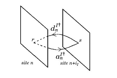
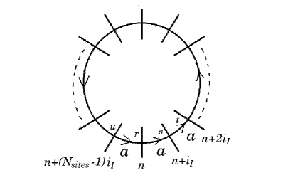
(a)	(b)

Figure 1: (a)The color charge for the state $|phys\ 1\rangle\equiv d^{I{\dagger}}_{n,rs}a^{I{\dagger}}_{n,sr}|0\rangle$. The planes represent the color space. $a_{n}^{I{\dagger}}$ carries color $r$ at site $n$ to $s$ at site $n+i_{I}$ and $d_{n}^{I{\dagger}}$ carries it back to $r$ at site $n$. (b) The color charge for the state $|phys\ 2\rangle\equiv a^{I{\dagger}}_{n+(N_{sites}-1)i_{I},ru}\cdots a^{I{\dagger}}_{n+i_{I},ts}a^{I{\dagger}}_{n,sr}|0\rangle$. The lines which intersect a circle represent the color planes at sites. The color goes all the way around the transverse lattice.

One also needs to be careful with operator ordering. One can show that the state $d^{I{\dagger}}_{n,rs}a^{I{\dagger}}_{n,st}b^{I{\dagger}}_{n,tr}|0\rangle$ is physical, while the state $b^{I{\dagger}}_{n,rs}a^{I{\dagger}}_{n,st}d^{I{\dagger}}_{n,tr}|0\rangle$ is unphysical. This statement is almost obvious when one recalls what each creation operator does.

We should however note that a true physical state be summed over all the transverse sites since we have discrete translational symmetry in the transverse direction. That is, for example, the states $d^{I{\dagger}}_{11,rs}a^{I{\dagger}}_{11,sr}|0\rangle$ and $d^{I{\dagger}}_{12,rs}a^{I{\dagger}}_{12,sr}|0\rangle$ are the same up to a phase factor given by $\exp(iP^{2}a)$. We set the phase factor to one since we take physical states to have $P^{1}=P^{2}=0$. The physical state $|phys\ 1\rangle$ is in fact $\sum_{i,j=1}^{N_{sites}}d^{I{\dagger}}_{ij,rs}a^{I{\dagger}}_{ij,sr}|0\rangle$ with the appropriate normalization constant. From a computational point of view this leads to a great simplification in the large $N_{c}$ limit. Because as shown in appendix A it turns out that in the large $N_{c}$ limit we can drop the site index $n$ from the expression of the supercharges and thus can practically set $N_{sites}=1$ for our calculation. This is in some sense the manifestation of the Eguchi-Kawai reduction [18]. Eguchi-Kawai reduction tells us in the usual lattice theory that the large $N_{c}$ limit allows us to work with only one site in each of the space-time directions in Euclidean space. However, the way we justify this reduction in our transverse lattice formulation is quite different from the way Eguchi and Kawai do in the usual lattice formulation. Therefore, we believe that we do not have to introduce quenching [19] or twisted [20] lattices to overcome the problem that the naive Eguchi-Kawai reduction comes across at weak couplings [19]. We refer the reader to appendix A for more detailed support for this claim.

Periodic conditions on the fields allow for physical states of the form $|phys\ 2\rangle\equiv\sum_{n}a^{I{\dagger}}_{n+(N_{sites}-1)i_{I},ru}\cdots a^{I{\dagger}}_{n+i_{I},ts}a^{I{\dagger}}_{n,sr}|0\rangle$. The color for this state is carried around the transverse lattice, as shown in Fig. 1b. We will refer to these states as cyclic states. The states where the color flux does not go all the way around the transverse lattice we will refer to as non-cyclic states. We characterize states by what we call the winding number defined by $W_{I}=n_{I}/N_{sites}$, where $n_{I}\equiv\sum_{n}(a_{n}^{I{\dagger}}a_{n}^{I}-d^{I{\dagger}}_{n}d_{n}^{I})$. For $N_{sites}=1$, the winding number $W_{I}$ simply gives us the excess number of $a^{I{\dagger}}$ over $d^{I{\dagger}}$ in a state. We use the winding number to classify states since the winding number is a good quantum number commuting with $P^{-}_{SDLCQ}$ as we will see in the next section. In the language of the winding number the non-cyclic states are those states with $W_{I}=0$ and cyclic states have non-zero $W_{I}$.

3 SDLCQ of the transverse lattice model

The transverse lattice formulation of ${\cal N}=1$ SYM theory in 3+1 dimension presented in the previous section has several undesirable features. First and foremost the naive Lagrangian suffers from the fermion species doubling problem [22]. Second, the supersymmetric structure of the theory is completely hidden. Lastly, the resulting Hamiltonian is $6^{th}$ order in the dynamical fields. From the numerical point of view a $6^{th}$ order interaction makes the theory considerably more difficult to solve. In Ref. [13] we found that the (2+1)–dimensional supersymmetric Hamiltonian is only $4^{th}$ order making this discrete formulation of the theory very different. Unfortunately, it seems this is not the case for 3+1 dimensional model. Instead we seem to have supersymmetric Hamiltonian of $8^{th}$ order in fields. However, since this SDLCQ Hamiltonian is free from the doubling problem [22] and since the supercharge $Q^{-}_{\alpha}$, where $\alpha=1,2$, is of $5^{th}$ order and it is this $Q^{-}_{\alpha}$ that we make use of for our calculations, we think that this SDLCQ formulation is still more advantageous than the naive DLCQ formulation. There can, of course, be many discrete formulations that correspond to the same continuum theory and it is therefore desirable to search for a better one.

In the spirit of SDLCQ we will attempt a discrete formulation based on the underlying super-algebra of this theory,

$$\{Q^{\pm}_{\alpha},Q^{\pm}_{\beta}\}=2\sqrt{2}P^{\pm}\delta_{\alpha\beta},\quad\{Q^{+}_{\alpha},Q^{-}_{\beta}\}=0,$$ (14)

where $\alpha,\beta=1,2$ and the supercharge $Q$ is given by

$$Q\equiv\sum_{n}\int dx^{-}j^{+}_{n}\equiv\left(\begin{array}[]{c}Q^{+}_{1}\\ Q^{+}_{2}\\ Q^{-}_{1}\\ Q^{-}_{2}\end{array}\right)$$

with $j^{\mu}_{n}$ being the supercurrent at the site $n=(i,j)$, which is a Majorana spinor. For the derivation of the super-algebra in Majorana representation Eq. (14), see the appendix B. We’ve set $P^{I}=0$ with $I=1,2$ since we’re considering the physical states only with $P^{I}=0$. Note that this choice of $P^{I}$ has made Eq. (14) coincide with the ${\cal N}$=2 super-algebra in 1+1 dimensions also known as ${\cal N}$=(2,2) super-algebra although we are considering ${\cal N}$=1 SYM in 3+1 dimensions.

In this effort however there are some fundamental limits to how far one can go. As we discussed in the previous section the physical states of this theory must conserve the color charge at every point on the transverse lattice. Experience with other supersymmetric theories indicates that each term in $Q^{+}_{\alpha}$ has to be either the product of one $M_{n}$ and one $\psi_{n}$ or of one $M_{n}^{{\dagger}}$ and one $\psi_{n}$ therefore $Q^{+}_{\alpha}$ is unphysical, by which we mean that $Q^{+}_{\alpha}$ transforms a physical state into an unphysical one, so that $\langle phys|Q^{+}_{\alpha}|phys\rangle=0$. While this is not a theorem, it seems very difficult to have any other structure since in light cone quantization $P^{+}$ is a kinematic operator and therefore independent of the coupling. There appears to be no way to make a physical $P^{+}$ from $Q^{+}_{\alpha}$. We will use $P^{+}$ as given in Eq. (7) in what follows. Similarly, we are not able to generally construct physical $P^{I}$ from $Q^{+}_{\alpha}$ and $Q^{-}_{\beta}$. In fact $P^{I}$ is unphysical in our formalism, leading to $\langle phys|P^{I}|phys\rangle=0$. Formally we will work in the frame where total $P^{I}$ is zero, so it would appear consistent with this result. We should note, however, that this is not totally satisfying because $P^{I}=0$ was a choice and a non-zero value is equally valid and not consistent with the matrix element.

Despite these difficulties we find a physical $Q^{-}_{\alpha}$ which gives us $P^{-}_{SDLCQ}\stackrel{{\scriptstyle a\to 0}}{{\longrightarrow}}P^{-}_{cont}$. The expression for $Q^{-}_{\alpha}$ is

$$Q_{\alpha}^{-} = i2^{3/4}a^{2}\sum_{n}\int dx^{-}{\rm tr}\Biggl{\{}\Bigg{[}\frac{-i}{2ga^{2}}\left(M_{n}^{I}\stackrel{{\scriptstyle\leftrightarrow}}{{\partial_{-}}}M_{n}^{I{\dagger}}+M_{n-i_{I}}^{I{\dagger}}\stackrel{{\scriptstyle\leftrightarrow}}{{\partial_{-}}}M_{n-i_{I}}^{I}\right)-2g\psi_{Rn}^{T}\psi_{Rn}\Bigg{]}$$

$$\times\frac{1}{\partial_{-}}(\sigma_{2}\psi_{Rn})_{\alpha}+\frac{-i}{2ga^{2}}(M_{n}^{I}M_{n+i_{I}}^{J}M_{n+i_{J}}^{I{\dagger}}M_{n}^{J{\dagger}}-1)(\beta_{I}\beta_{J}\sigma_{2}\psi_{Rn})_{\alpha}\Biggr{\}}$$

$$\stackrel{{\scriptstyle a\to 0}}{{\longrightarrow}}i2^{-1/4}\int d^{3}x\left\{-2gJ^{+}\frac{1}{\partial_{-}}(\sigma_{2}\psi_{R})_{\alpha}+F_{IJ}(\beta_{I}\beta_{J}\sigma_{2}\psi_{R})_{\alpha}\right\},$$

where $\beta_{1}\equiv\sigma_{1}$, $\beta_{2}=\sigma_{3}$, $gJ^{+}\equiv ig[A_{I},\partial_{-}A_{I}]+\partial_{I}\partial_{-}A_{I}+2g\psi_{R}\psi_{R}$, and the last line is the continuum form for $Q^{-}_{\alpha}$ in 3+1 dimensions.

It is tedious but straightforward to check that $\{Q^{-}_{1},Q^{-}_{1}\}\neq\{Q^{-}_{2},Q^{-}_{2}\}$, while both $\{Q^{-}_{1},Q^{-}_{1}\}$ and $\{Q^{-}_{2},Q^{-}_{2}\}$ give the same correct $P^{-}$ in the limit of $a\to 0$. In addition, one can show that $\{Q^{-}_{1},Q^{-}_{2}\}\neq 0$ in the discrete form but becomes zero as $a\to 0$. This means that we preserve only one supersymmetry algebra, say $\{Q^{-}_{1},Q^{-}_{1}\}=P^{-}$, in our discrete formalism. We cannot use both $Q^{-}_{1}$ and $Q^{-}_{2}$ at the same time to construct physical states since they do not commute with each other. However, both $Q^{-}_{1}$ and $Q^{-}_{2}$ separately give us the same mass spectrum when we perform SDLCQ calculations. Thus, it is suffice to consider only one of the two and we take $Q^{-}_{1}$ for our calculations in the following sessions.

Notice that $Q^{-}_{\alpha}$ above is fifth order and, thus, $P^{-}_{SDLCQ}$ obtained from it is eighth order in fields as we mentioned at the beginning of this section. In fact we find

$$P^{-}_{SDLCQ}\equiv\frac{\{Q_{1}^{-},Q_{1}^{-}\}}{2\sqrt{2}}$$

$$=a^{2}\sum_{n}\int dx{\rm tr}\Bigg{\{}-\frac{g^{2}}{2}\frac{i}{2g^{2}a^{2}}\left[\left(M_{n}^{I}\stackrel{{\scriptstyle\leftrightarrow}}{{\partial}}M_{n}^{I{\dagger}}+M_{n-i_{I}}^{I{\dagger}}\stackrel{{\scriptstyle\leftrightarrow}}{{\partial}}M_{n-i_{I}}^{I}\right)+2u^{\alpha}_{n}u^{\alpha}_{n}\right]$$

$$\qquad\times\frac{1}{\partial^{2}}\frac{i}{2g^{2}a^{2}}\left[\left(M_{n}^{I}\stackrel{{\scriptstyle\leftrightarrow}}{{\partial}}M_{n}^{I{\dagger}}+M_{n-i_{I}}^{I{\dagger}}\stackrel{{\scriptstyle\leftrightarrow}}{{\partial}}M_{n-i_{I}}^{I}\right)+2u^{\alpha}_{n}u^{\alpha}_{n}\right]$$

$$-\frac{i}{2a^{2}}(u^{2}_{n+i_{I}}M_{n}^{I{\dagger}}-M_{n}^{I{\dagger}}u^{2}_{n})\partial^{-1}(M_{n}^{I}u^{2}_{n+i_{I}}-u^{2}_{n}M_{n}^{I})+\frac{i}{2a^{2}}\Big{\{}$$

$$(u^{2}_{n+i_{1}+i_{2}}M_{n+i_{2}}^{1{\dagger}}-M_{n+i_{2}}^{1{\dagger}}u^{2}_{n+i_{2}})\partial^{-1}(M_{n}^{2{\dagger}}u^{1}_{n}M_{n}^{1}M_{n+i_{1}}^{2}-u^{1}_{n+i_{2}}M_{n+i_{2}}^{2}M_{n+2i_{2}}^{1}M_{n+i_{1}+i_{2}}^{2{\dagger}})$$

$$+(u^{2}_{n+i_{2}}M_{n}^{2{\dagger}}-M_{n}^{2{\dagger}}u^{2}_{n})\partial^{-1}(u^{1}_{n}M_{n}^{1}M_{n+i_{1}}^{2}M_{n+i_{2}}^{1{\dagger}}-M_{n-i_{1}}^{1{\dagger}}u^{1}_{n-i_{1}}M_{n-i_{1}}^{2}M_{n-i_{1}+i_{2}}^{1})$$

$$+(u^{2}_{n+i_{1}}M_{n+i_{1}}^{2}-M_{n+i_{1}}^{2}u^{2}_{n+i_{1}+i_{2}})\partial^{-1}(M_{n+i_{2}}^{1{\dagger}}M_{n}^{2{\dagger}}u^{1}_{n}M_{n}^{1}-M_{n+i_{1}+i_{2}}^{1}M_{n+2i_{1}}^{2{\dagger}}M_{n+i_{1}}^{1{\dagger}}u^{1}_{n+i_{1}})$$

$$+(u^{2}_{n}M_{n}^{1}-M_{n}^{1}u^{2}_{n+i_{1}})\partial^{-1}(M_{n+i_{1}}^{2}M_{n+i_{2}}^{1{\dagger}}M_{n}^{2{\dagger}}u^{1}_{n}-M_{n+i_{1}-i_{2}}^{2{\dagger}}M_{n-i_{2}}^{1{\dagger}}u^{1}_{n-i_{2}}M_{n-i_{2}}^{2})\Big{\}}$$

$$-\frac{i}{4a^{2}}\Bigl{\{}(M_{n+i_{1}}^{2}M_{n+i_{2}}^{1{\dagger}}M_{n}^{2{\dagger}}u^{1}_{n}-M_{n+i_{1}-i_{2}}^{2{\dagger}}M_{n-i_{2}}^{1{\dagger}}u^{1}_{n-i_{2}}M_{n-i_{2}}^{2})$$

$$\times\partial^{-1}(u^{1}_{n}M_{n}^{2}M_{n+i_{2}}^{1}M_{n+i_{1}}^{2{\dagger}}-M_{n-i_{2}}^{2{\dagger}}u^{1}_{n-i_{2}}M_{n-i_{2}}^{1}M_{n+i_{1}-i_{2}}^{2})$$

$$+(M_{n}^{2{\dagger}}u^{1}_{n}M_{n}^{1}M_{n+i_{1}}^{2}-u^{1}_{n+i_{2}}M_{n+i_{2}}^{2}M_{n+2i_{2}}^{1}M_{n+i_{1}+i_{2}}^{2{\dagger}})$$

$$\times\partial^{-1}(M_{n+i_{1}}^{2{\dagger}}M_{n}^{1{\dagger}}u^{1}_{n}M_{n}^{2}-M_{n+i_{1}+i_{2}}^{2}M_{n+2i_{2}}^{1{\dagger}}M_{n+i_{2}}^{2{\dagger}}u^{1}_{n+i_{2}})$$

$$+(M_{n+i_{2}}^{1{\dagger}}M_{n}^{2{\dagger}}u^{1}_{n}M_{n}^{1}-M_{n+i_{1}+i_{2}}^{1}M_{n+2i_{1}}^{2{\dagger}}M_{n+i_{1}}^{1{\dagger}}u^{1}_{n+i_{1}})$$

$$\times\partial^{-1}(M_{n}^{1{\dagger}}u^{1}_{n}M_{n}^{2}M_{n+i_{2}}^{1}-u^{1}_{n+i_{1}}M_{n+i_{1}}^{1}M_{n+2i_{1}}^{2}M_{n+i_{1}+i_{2}}^{1{\dagger}})$$

$$+(u^{1}_{n}M_{n}^{1}M_{n+i_{1}}^{2}M_{n+i_{2}}^{1{\dagger}}-M_{n-i_{1}}^{1{\dagger}}u^{1}_{n-i_{1}}M_{n-i_{1}}^{2}M_{n-i_{1}+i_{2}}^{1}$$

$$\times\partial^{-1}(M_{n+i_{2}}^{1}M_{n+i_{1}}^{2{\dagger}}M_{n}^{1{\dagger}}u^{1}_{n}-M_{n-i_{1}+i_{2}}^{1{\dagger}}M_{n-i_{1}}^{2{\dagger}}u^{1}_{n-i_{1}}M_{n-i_{1}}^{1})\Big{\}}$$

$$+\frac{-1}{8a^{2}}(M_{n}^{1}M_{n+i_{1}}^{2}M_{n+i_{2}}^{1{\dagger}}M_{n}^{2{\dagger}}-M_{n}^{2}M_{n+i_{2}}^{1}M_{n+i_{1}}^{2{\dagger}}M_{n}^{1{\dagger}})^{2}\Bigg{\}}.$$

One can show that by setting $g=0$ and $M,M^{{\dagger}}=1$ this $P^{-}_{SDLCQ}$ gives rise to a dispersion relation

$$k^{-}=\frac{1}{2k^{+}}\left[\left(\frac{\sin\frac{k^{1}a}{2}}{a/2}\right)^{2}+\left(\frac{\sin\frac{k^{2}a}{2}}{a/2}\right)^{2}\right],$$

which is free from the fermion species doubling problem [22]. Furthermore, one can check that this $Q^{-}$ commutes with $P^{+}$ obtained from ${\cal L}$; $[Q^{-},P^{+}]=0$. Thus, it follows that,

$$\langle phys|[Q^{-},M^{2}]|phys\rangle=\langle phys|[Q^{-},2P^{+}P^{-}_{SDLCQ}]|phys\rangle=0$$ (15)

in our SDLCQ formalism, where $M^{2}\equiv 2P^{+}P^{-}_{SDLCQ}-(P^{1})^{2}-(P^{2})^{2}$. The fact that the Hamiltonian is the square of a supercharge will guarantee the usual supersymmetric degeneracy of the massive spectrum, and our numerical solutions will substantiate this. Unfortunately one needs a $Q^{+}$ to guarantee the degeneracy of the massless bound states.

Recalling that we set $N_{sites}=1$ in both transverse directions and that we are in the large-$N_{c}$ limit. we can write $Q^{-}_{1}$ as

$$Q^{-}_{1}={\cal Q}^{-}_{11}+{\cal Q}^{-}_{12}+{\cal Q}^{-}_{13},$$

where

$${\cal Q}^{-}_{11}=-\frac{i2^{-1/4}a^{2}g}{\sqrt{\pi}}\int_{0}^{\infty}dk_{1}dk_{2}dk_{3}\delta(k_{1}+k_{2}-k_{3})$$

$$\times\Big{[}\frac{k_{2}-k_{1}}{k_{3}\sqrt{k_{1}k_{2}}}(-b^{2{\dagger}}d^{I}a^{I}+d^{I{\dagger}}a^{I{\dagger}}b^{2}-b^{2{\dagger}}a^{I}d^{I}+a^{I{\dagger}}d^{I{\dagger}}b^{2})$$

$$+\frac{k_{2}+k_{3}}{k_{1}\sqrt{k_{2}k_{3}}}(-d^{I{\dagger}}b^{2}d^{I}+b^{2{\dagger}}d^{I{\dagger}}d^{I}-a^{I{\dagger}}b^{2}a^{I}+b^{2{\dagger}}a^{I{\dagger}}a^{I})$$

$$+\frac{k_{3}+k_{1}}{k_{2}\sqrt{k_{3}k_{1}}}(a^{I{\dagger}}a^{I}b^{2}-a^{I{\dagger}}b^{2{\dagger}}a^{I}+d^{I{\dagger}}d^{I}b^{2}-d^{I{\dagger}}b^{2{\dagger}}d^{I})$$

$$+\left(\frac{1}{k_{1}}+\frac{1}{k_{2}}-\frac{1}{k_{3}}\right)(b^{2{\dagger}}b^{2{\dagger}}b^{2}+b^{2{\dagger}}b^{2}b^{2})\Big{]},$$ (16)

$${\cal Q}^{-}_{12}=-\frac{i2^{-1/4}a^{2}g}{\sqrt{\pi}}\int_{0}^{\infty}dk_{1}dk_{2}dk_{3}\delta(k_{1}+k_{2}-k_{3})$$

$$\times\Big{[}\frac{-1}{k_{3}}(b^{2{\dagger}}b^{1}b^{1}+b^{1{\dagger}}b^{1{\dagger}}b^{2})+\frac{1}{k_{1}}(b^{1{\dagger}}b^{2}b^{1}+b^{2{\dagger}}b^{1{\dagger}}b^{1})+\frac{1}{k_{2}}(b^{1{\dagger}}b^{2{\dagger}}b^{1}+b^{1{\dagger}}b^{1}b^{2})\Big{]},$$ (17)

$${\cal Q}^{-}_{13}=-\frac{i2^{-1/4}a^{2}g}{\sqrt{\pi}}\frac{a^{2}g^{2}}{4\pi}\int_{0}^{\infty}dk_{1}dk_{2}dk_{3}dk_{4}dk_{5}\Big{\{}\delta(k_{1}+k_{2}+k_{3}+k_{4}-k_{5})\Big{[}$$

$$\frac{1}{\sqrt{k_{1}k_{2}k_{3}k_{4}}}(b^{1{\dagger}}d^{1}d^{2}a^{1}a^{2}+d^{2{\dagger}}d^{1{\dagger}}a^{2{\dagger}}a^{1{\dagger}}b^{1}-b^{1{\dagger}}d^{2}d^{1}a^{2}a^{1}-d^{1{\dagger}}d^{2{\dagger}}a^{1{\dagger}}a^{2{\dagger}}b^{1})$$

$$+\frac{1}{\sqrt{k_{2}k_{3}k_{4}k_{5}}}(d^{2{\dagger}}b^{1}d^{1}d^{2}a^{1}+b^{1{\dagger}}d^{2{\dagger}}d^{1{\dagger}}a^{2{\dagger}}d^{1}-d^{1{\dagger}}b^{1}d^{2}d^{1}a^{2}-b^{1{\dagger}}d^{1{\dagger}}d^{2{\dagger}}a^{1{\dagger}}d^{2})$$

$$+\frac{1}{\sqrt{k_{3}k_{4}k_{5}k_{1}}}(d^{1{\dagger}}a^{2}b^{1}d^{1}d^{2}+a^{1{\dagger}}b^{1{\dagger}}d^{2{\dagger}}d^{1{\dagger}}d^{2}-d^{2{\dagger}}a^{1}b^{1}d^{2}d^{1}-a^{2{\dagger}}b^{1{\dagger}}d^{1{\dagger}}d^{2{\dagger}}d^{1})$$

$$+\frac{1}{\sqrt{k_{4}k_{5}k_{1}k_{2}}}(a^{2{\dagger}}a^{1}a^{2}b^{1}d^{1}+a^{2{\dagger}}a^{1{\dagger}}b^{1{\dagger}}d^{2{\dagger}}a^{1}-a^{1{\dagger}}a^{2}a^{1}b^{1}d^{2}-a^{1{\dagger}}a^{2{\dagger}}b^{1{\dagger}}d^{1{\dagger}}a^{2})$$

$$+\frac{1}{\sqrt{k_{5}k_{1}k_{2}k_{3}}}(a^{1{\dagger}}d^{2}a^{1}a^{2}b^{1}+d^{1{\dagger}}a^{2{\dagger}}a^{1{\dagger}}b^{1{\dagger}}a^{2}-a^{2{\dagger}}d^{1}a^{2}a^{1}b^{1}-d^{2{\dagger}}a^{1{\dagger}}a^{2{\dagger}}b^{1{\dagger}}a^{1})\Big{]}$$

$$+\delta(k_{1}+k_{2}+k_{3}-k_{4}-k_{5})$$

$$\times\Big{[}\frac{1}{\sqrt{k_{1}k_{2}k_{3}k_{4}}}(d^{1{\dagger}}a^{2{\dagger}}a^{1{\dagger}}a^{2}b^{1}+a^{1{\dagger}}b^{1{\dagger}}d^{2}a^{1}a^{2}-d^{2{\dagger}}a^{1{\dagger}}a^{2{\dagger}}a^{1}b^{1}-a^{2{\dagger}}b^{1{\dagger}}d^{1}a^{2}a^{1})$$

$$+\frac{1}{\sqrt{k_{2}k_{3}k_{4}k_{5}}}(b^{1{\dagger}}d^{2{\dagger}}d^{1{\dagger}}d^{1}d^{2}+d^{2{\dagger}}d^{1{\dagger}}b^{1}d^{1}d^{2}-b^{1{\dagger}}d^{1{\dagger}}d^{2{\dagger}}d^{2}d^{1}-d^{1{\dagger}}d^{2{\dagger}}b^{1}d^{2}d^{1})$$

$$+\frac{1}{\sqrt{k_{3}k_{4}k_{5}k_{1}}}(a^{1{\dagger}}b^{1{\dagger}}d^{2{\dagger}}d^{2}a^{1}+d^{1{\dagger}}a^{2{\dagger}}a^{2}b^{1}d^{1}-a^{2{\dagger}}b^{1{\dagger}}d^{1{\dagger}}d^{1}a^{2}-d^{2{\dagger}}a^{1{\dagger}}a^{1}b^{1}d^{2})$$

$$+\frac{1}{\sqrt{k_{4}k_{5}k_{1}k_{2}}}(a^{2{\dagger}}a^{1{\dagger}}b^{1{\dagger}}a^{1}a^{2}+a^{2{\dagger}}a^{1{\dagger}}a^{1}a^{2}b^{1}-a^{1{\dagger}}a^{2{\dagger}}b^{1{\dagger}}a^{2}a^{1}-a^{1{\dagger}}a^{2{\dagger}}a^{2}a^{1}b^{1})$$

$$+\frac{1}{\sqrt{k_{5}k_{1}k_{2}k_{3}}}(d^{2{\dagger}}d^{1{\dagger}}a^{2{\dagger}}b^{1}d^{1}+b^{1{\dagger}}d^{2{\dagger}}d^{1}d^{2}a^{1}-d^{1{\dagger}}d^{2{\dagger}}a^{1{\dagger}}b^{1}d^{2}-b^{1{\dagger}}d^{1{\dagger}}d^{2}d^{1}a^{2})\Big{]}\Big{\}},$$ (18)

with $k^{+}\equiv k$, $a_{1}\equiv a(k_{1})$, $a^{{\dagger}}aa\equiv{\rm tr}(a^{{\dagger}}_{3}a_{1}a_{2})$, $a^{{\dagger}}a^{{\dagger}}a\equiv{\rm tr}(a^{{\dagger}}_{1}a^{{\dagger}}_{2}a_{3})$, $a^{{\dagger}}aaaa\equiv{\rm tr}(a^{{\dagger}}_{5}a_{1}a_{2}a_{3}a_{4})$, $a^{{\dagger}}a^{{\dagger}}a^{{\dagger}}a^{{\dagger}}a\equiv{\rm tr}(a^{{\dagger}}_{1}a^{{\dagger}}_{2}a^{{\dagger}}_{3}a^{{\dagger}}_{4}a_{5})$, $a^{{\dagger}}a^{{\dagger}}a^{{\dagger}}aa\equiv{\rm tr}(a^{{\dagger}}_{1}a^{{\dagger}}_{2}a^{{\dagger}}_{3}a_{4}a_{5})$, and $a^{{\dagger}}a^{{\dagger}}aaa\equiv{\rm tr}(a^{{\dagger}}_{4}a^{{\dagger}}_{5}a_{1}a_{2}a_{3})$. ${\cal Q}_{11}$ is the part of $Q^{-}_{1}$ which looks exactly like $Q^{-}$ in 2+1 dimensional model with the difference being that here we have two types for each of the bosonic fields $a$ and $d$. ${\cal Q}_{12}$ is a new piece in 3+1 dimensions and mixes two different types of fermionic fields. ${\cal Q}_{13}$ is also new and composed of fields of fifth order. Note that for small couplings, ${\cal Q}_{11}$ and ${\cal Q}_{12}$ dominate over ${\cal Q}_{13}$, while ${\cal Q}_{13}$ dominates in the strong coupling regime. Notice that from this explicit expression for $Q^{-}_{1}$ it is clear that the winding number introduced in the last section evidently commutes with $Q^{-}_{1}$ and, thus, with $P^{-}_{SDLCQ}$. Therefore, cyclic states do not mix with non-cyclic states.

It is always important to look for symmetries of $Q^{-}$ since the symmetries, if any, will reduce the amount of the computational efforts considerably. To do this, let us consider three cases separately: (i) the intermediate coupling where we have all the three pieces together for $Q^{-}_{1}$; (ii) the weak coupling limit where we can ignore ${\cal Q}_{13}$; (iii) the strong coupling limit where we consider ${\cal Q}_{13}$ only. For the first case (i) we find two $Z_{2}$ symmetries,

• $a^{1}_{ij}\leftrightarrow-a^{2}_{ij},\ d^{1}_{ij}\leftrightarrow-d^{2}_{ij},\ b^{1}_{ij}\leftrightarrow-b^{1}_{ij},\ b^{2}\ {\rm unchanged}$,

• $a^{I}_{ij}\leftrightarrow-d^{I}_{ji},\ b^{\alpha}_{ij}\leftrightarrow-b^{\alpha}_{ji}$.

The first symmetry implies that states with the winding numbers, say $(W_{1},W_{2})$, are equivalent to those with $(W_{2},W_{1})$ up to the minus sign. On the other hand the second symmetry implies that states with $(W_{1},W_{2})$ are equivalent to those with $(-W_{1},-W_{2})$ up to the minus sign.

In the case of the weak coupling limit (ii), we find two more independent $Z_{2}$ symmetries;

• $a^{I}_{ij}\leftrightarrow-a^{I}_{ji},\ d^{I}_{ij}\leftrightarrow-d^{I}_{ji},\ b^{\alpha}_{ij}\leftrightarrow-b^{\alpha}_{ji}$.

• $a^{1}_{ij}\leftrightarrow-d^{1}_{ji},\ a^{2}_{ij}\leftrightarrow-a^{2}_{ji},\ d^{2}_{ij}\leftrightarrow-d^{2}_{ji},\ b^{\alpha}_{ij}\leftrightarrow-b^{\alpha}_{ji}$.

The second of these implies, with the help of the second $Z_{2}$ symmetry we found in the case of (i), the equivalence of states under $(W_{1},W_{2})\leftrightarrow(-W_{1},W_{2})\leftrightarrow(W_{1},-W_{2})$.

In the strong coupling limit (iii), we do not have any other $Z_{2}$ symmetries besides the two we found in the case of (i). However, it is easy to see that ${\cal Q}_{13}$ commutes with $b^{2{\dagger}}b^{2}$, thus the number of $b^{2{\dagger}}$’s is a good quantum number as well as the two winding numbers.

It is interesting to see what we can find for each of the three different cases (i), (ii) and (iii). However, in this our first attempt to formulate ${\cal N}=(2,2)$ SYM in 3+1 dimensions with SDLCQ on a two dimensional transverse lattice, we constrain ourselves to consider only the most generic case (i) where we have all the three pieces together for $Q^{-}$.

Now we are in a position to solve the eigenvalue problem $2P^{+}P^{-}_{SDLCQ}|phys\rangle=m^{2}|phys\rangle$. We impose the periodicity condition on $M^{I}_{n}$, $M^{I{\dagger}}_{n}$ and $u^{\alpha}_{n}$ in the $x^{-}$ direction giving a discrete spectrum for $k^{+}$, and ignore the zero-mode:

$$k^{+}=\frac{\pi}{L}n\quad(n=1,2,\ldots.),\qquad\int_{0}^{\infty}dk^{+}\rightarrow\frac{\pi}{L}\sum_{n=1}^{\infty}.$$

We impose a cut-off on the total longitudinal momentum $P^{+}$ i.e. $P^{+}=\pi K/L$, where $K$ is an integer also known as the ‘harmonic resolution’, which indicates the coarseness of our numerical results. For a fixed $P^{+}$ i.e. a fixed $K$, the number of partons in a state is limited up to the maximum, that is $K$, so that the total number of Fock states is finite, and, therefore, we have reduced the infinite dimensional eigenvalue problem to a finite dimensional one.

For this initial study of the transverse lattice we consider resolution up to $K=8$ for non-cyclic ($W_{1}=W_{2}=0$) states and up to $K=W_{I}+6$ and $K=W_{I}+5$ for states with $|W_{I}|=1$ and $|W_{I}|=2,3,4,5$, respectively. We were able to handle these calculations with our SDLCQ Mathematica code and $C++$ code.

4 Coupling dependence of the mass spectrum

In this section we will discuss the mass spectrum as a function of $g^{\prime}\equiv g\sqrt{N_{c}}$ for $K=4,5,6$.

It is instructive to see the dependence of $m^{2}$ on the coupling since we have terms in $Q^{-}$ that go like $g^{\prime}$ and $g^{\prime 3}$. In Fig. 2 we show the entire mass spectrum of non-cyclic states in units of $g^{\prime 2}/\pi a^{2}$ for $K=4,5,6$ as a function of $g^{\prime}$ in a log-log plot. In order to see the crossings in more detail we show Fig. 2(b), (d), and (f) on a different scale from (a), (c) and (e), respectively. We’ve set $10^{-8}$ or less to the numerical zero in our code.

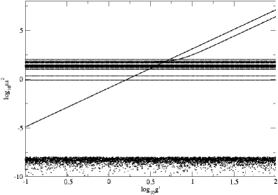
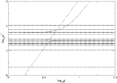
(a)	(b)
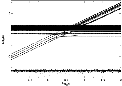
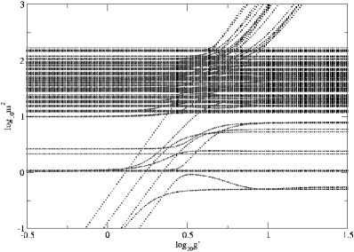
(c)	(d)
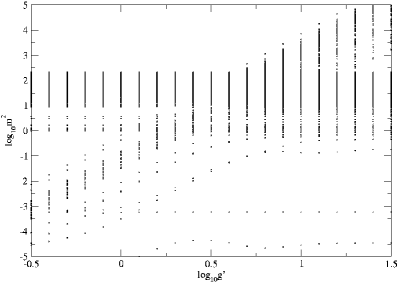
(e)	(f)

Figure 2: Log-log plots of the mass spectrum $m^{2}$ in units of $\frac{g^{\prime 2}}{\pi a^{2}}$ versus $g^{\prime}\equiv g\sqrt{N_{c}}$ with $K=4,5,6$ for (a),(c),(e), respectively. (b), (d), and (f) are the same as (a), (c) and (e), respectively but on a different scale so that one can see the crossings in more detail. $10^{-8}$ or less is the numerical zero in our code.

As one can see from Fig. 2, there is a rich structure in the mass spectrum as a function of $g^{\prime}$, and the origin of this structure for the case where $K=4$ in Fig. 2(a) and (b) is rather easy to understand. We find four types of states; (i) those states which are killed by ${\cal Q}_{13}$ and whose $m^{2}$ in units of $\frac{g^{\prime 2}}{\pi a^{2}}$ are independent of $g^{\prime}$; (ii) those states which vanish upon the action of ${\cal Q}_{11}+{\cal Q}_{12}$ and thus whose $m^{2}$ in units of $\frac{g^{\prime 2}}{\pi a^{2}}$ go like $g^{\prime 4}$; (iii) those states which survive upon the action of ${\cal Q}_{11}+{\cal Q}_{12}$ and of ${\cal Q}_{13}$ independently and whose $m^{2}$ in units of $\frac{g^{\prime 2}}{\pi a^{2}}$ go like $(A+Bg^{\prime 2})^{2}$, where $A,B$ are some constants; (iv) those massless states which become zero upon the action of ${\cal Q}_{11}+{\cal Q}_{12}+{\cal Q}_{13}$. From Fig. 2(a) and (b) it is easy to identify one state each for the second and third type because $m^{2}$ of a state of the second type go like $g^{\prime 4}$, giving rise to a straight line with a non-zero slope for all $g^{\prime}$ in the log-log plot, while $m^{2}$ for the third type is $(A+Bg^{\prime 2})^{2}$, leading to some flat, constant line at small $g^{\prime}$ and a (inclined) straight line at large $g^{\prime}$. We should note that for the second kind one should take into account the level crossing. The rest of the states clearly fall into either the first kind or the fourth kind. States of the first type yield $g^{\prime}$-independent $m^{2}$, thus, a flat line in the log-log plot, while states of the fourth type are massless represented by the “dots” below the line of $\log_{10}m^{2}=-8$ since the numerical zero is set to $10^{-8}$ in our code.

This discussion does not however seem to explain the dependence on $g^{\prime}$ of the mass spectrum with $K=5,6$. To get the full understanding of the behavior, we made a toy model. In this model we have a $2\times 2$ matrix $R$ for the boson sector of $Q^{-}$ given by

$$R=\left(\begin{array}[]{cc}b_{1}+c_{1}g^{\prime 2}&b_{2}+c_{2}g^{\prime 2}\\ b_{3}+c_{3}g^{\prime 2}&b_{4}+c_{4}g^{\prime 2}\end{array}\right),$$

where $b_{i}$ with $i=1,2,3,4$ is equal to either 0 or 1 and $c_{i}$ is equal to either 0 or $1/4\pi$. Here one should notice that we’ve factored out $g^{\prime}$ from $R$ or $Q^{-}$, and therefore $g^{\prime 2}$ from $P^{-}$. The $Q^{-}$ for this toy model is thus given by

$$Q^{-}/g^{\prime}=\left(\begin{array}[]{cc}0&R\\ R^{T}&0\end{array}\right),$$

where $T$ stands for the transpose. Thus, the matrix to diagonalize is

$$(Q^{-}/g^{\prime})^{2}=\left(\begin{array}[]{cc}RR^{T}&0\\ 0&R^{T}R\end{array}\right),$$

or equivalently $RR^{T}$. Among the $2^{8}=256$ possible forms for $Q^{-}$, we found sets of parameters that lead to a level crossing, and non-trivial behaviors in the mass spectrum. Some of those non-trivial ones look the same as some of those in Fig. 2, while there are others which do not look like any of those in Fig. 2. For example see Fig. 3, where Fig. 3(a) and (b) are the ones that we can see in the actual spectrum in Fig. 2, while 3(c) and (d) are not. The sets of parameters we used are given in Table 1. Of course there are ones which are seen in Fig. 2, but cannot be found in our toy model. However, it is very likely that as we increase the size of the matrix $R$ of our toy model, we would be able to identify those not-yet-seen behaviors in our toy model as well.

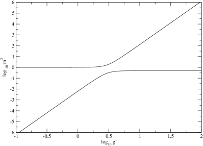
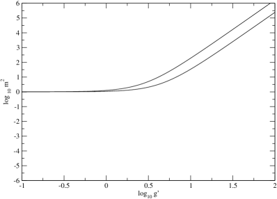
(a)	(b)
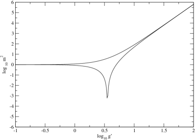
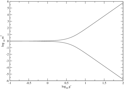
(c)	(d)

Figure 3: Sample spectra obtained from our toy model. (a) and (b) can be seen in the actual full spectrum in Fig. 2, while (c) and (d) cannot.

	$b_{1}$	$c_{1}$	$b_{2}$	$c_{2}$	$b_{3}$	$c_{3}$	$b_{4}$	$c_{4}$
Fig. 3(a)	0	$1/4\pi$	0	$1/4\pi$	1	0	0	0
Fig. 3(b)	0	0	1	$1/4\pi$	1	$1/4\pi$	0	$1/4\pi$
Fig. 3(c)	0	0	1	0	1	0	0	$1/4\pi$
Fig. 3(d)	0	$1/4\pi$	1	0	1	0	0	$1/4\pi$

Table 1: Parameter sets used for our toy model to get each of the spectra in Fig. 3.

Using this toy model, we can study wavefunction dependence on the coupling $g^{\prime}$. As the simplest example, consider the case of the level crossing shown in Fig. 3(a). In this case we can think of a bound state $|m^{2}\rangle$ as a linear combination of two different states,

$$|m^{2}\rangle=f(g^{\prime})|1\rangle+h(g^{\prime})|2\rangle,$$

where $f(g^{\prime})$ and $h(g^{\prime})$ are wavefunctions, which depend on $g^{\prime}$. $|1\rangle$ is a state of the first type of the four we considered above and responsible for the constant behavior of the mass spectrum and $|2\rangle$ is a state of the second type responsible for the $g^{\prime 4}$-behavior. In Fig. 3(a) the higher energy state stays constant for small $g^{\prime}$, where $f(g^{\prime})\gg h(g^{\prime})$, and goes like $g^{\prime 4}$ for large $g^{\prime}$, where $h(g^{\prime})\gg f(g^{\prime})$. The opposite behavior of the wavefunctions is true for the lower energy state. That is, the lower energy state goes like $g^{\prime 4}$ for small $g^{\prime}$, where $h(g^{\prime})\gg f(g^{\prime})$, and stays flat for large $g^{\prime}$, with $f(g^{\prime})\gg h(g^{\prime})$. This observation implies that for more general cases a bound state is a linear combination of states of the four types associated with $g^{\prime}$-dependent wavefunctions, and it is the non-trivial $g^{\prime}$-dependence of the wavefunctions that gives rise to such a rich, complicated spectrum in Fig. 2.

We expect that the structure of the mass spectrum as a function of $g^{\prime}$ will persist for the cyclic states and in fact we have numerically confirmed the similar structure for them as well.

Note that since the dominant structure of a bound state changes as one changes $g^{\prime}$, there is some sort of “transition” as one goes from weak coupling to strong coupling. It is of great interest to see if the winding number dependence of the mass spectrum varies due to this transition. We are not able to identify any states in strong coupling regime because of the rich and complicated behavior of the spectrum although we are able to find some states in the intermediate region where $g^{\prime}=1$.

We discuss the mass spectrum of the cyclic states as a function of the winding number and the resolution with $g^{\prime}=1$ in more detail in the next section. The discussion of the mass spectrum of the non-cyclic states is in the following section.

5 Numerical results for the cyclic $(W_{I}\neq 0)$ bound states

In principle we can study the case where both of the winding numbers are non-zero and the case where one of them equals zero. However, the size of the Fock basis is much larger for the former case than for the latter. This means that we can reach a higher resolution for the latter case. Thus, in order to get enough data to analyze for our first attempt we restrict ourselves to the case where we set one of the winding numbers to zero. Since we have two $Z_{2}$ symmetries, $(W_{1},W_{2})\leftrightarrow(W_{2},W_{1})$ and $(W_{1},W_{2})\leftrightarrow(-W_{1},-W_{2})$, we can set $W_{2}=0$ without loss of generality and consider only positive $W_{1}$ when studying the winding number dependence of the bound states.

As guaranteed by the super–algebra, we find numerically a degeneracy in the mass spectrum between massive fermionic and bosonic states. However, this supersymmetry is broken for the massless states since we do not preserve the entire set of super symmetry algebra. In this section we only consider the massive bound states, and therefore it suffices to consider only bosonic states.

In Fig. 4(a), (b), (c), and (d) we give plots of $m^{2}$ with $g^{\prime}=1$ for four low–energy bound states as a function of $1/(K-W_{1})$ and extrapolate $m^{2}_{\infty}$ in the $(K-W_{1})\to\infty$ limit using a linear fit $b+c/(K-W_{1})$ for (a) through (c) and a quadratic fit $b+c/(K-W_{1})+d/(K-W_{1})^{2}$ for (d), where $b,c,d$ are fitting parameters. We identify a bound state with different $K$’s from the properties of the bound state, such as the averaged number of partons of a particular type etc. We present here four bound states we could easily identify. The dominate fock component of the bound state in (a) and (c) has the form $b^{1{\dagger}}a^{1{\dagger}}\cdots a^{1{\dagger}}b^{1{\dagger}}$. For the bound state in (b) the dominant component is of the form $b^{1{\dagger}}a^{1{\dagger}}\cdots a^{1{\dagger}}b^{2{\dagger}}$. The bound state in (d) has the dominant component of $d^{2{\dagger}}a^{1{\dagger}}\cdots a^{1{\dagger}}a^{2{\dagger}}$.

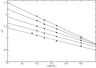
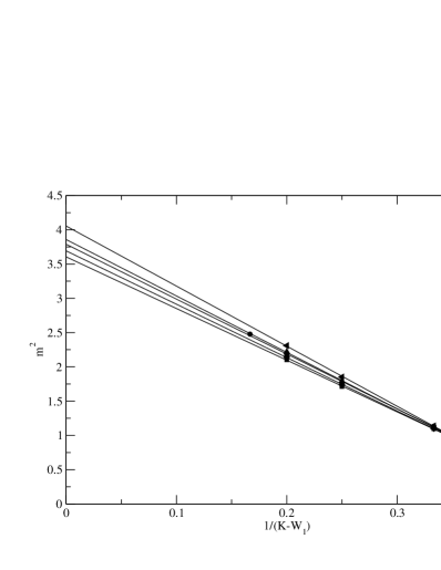
(a)	(b)
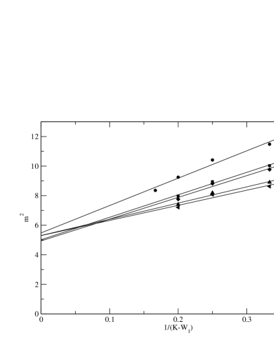
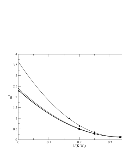
(c)	(d)

Figure 4: Plots of $m^{2}$ in units of $\frac{g^{\prime 2}}{\pi a^{2}}$ of low-energy cyclic bound states versus $1/(K-W_{1})$ for $W_{1}$=1(circle), 2(square), 3(diamond), 4(triangle up), 5(triangle left). Also shown are a linear fit for (a), (b), and (c) and a quadratic fit for (d). The coupling $g^{\prime}\equiv g\sqrt{N_{c}}=1$.

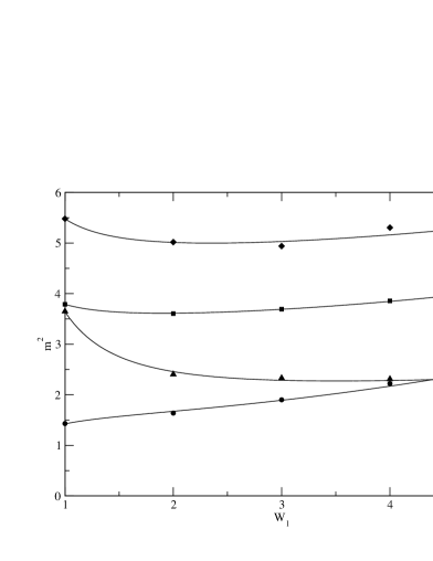
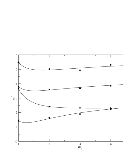
(a)	(b)

Figure 5: Plots of $K\to\infty$ limit of $m^{2}$ in units of $\frac{g^{\prime 2}}{\pi a^{2}}$ of low energy cyclic bound states versus $W_{1}$ with a fit to the data of the form $b+cW_{1}^{2}+d/W_{1}^{2}$ in (a) and of the form $b+c/W_{1}+d/W_{1}^{2}$ in (b). The circles correspond to the bound state in Fig. 4(a), squares in 4(b), diamonds in 4(c), and triangles in 4(d).

In Fig. 5 we present $m^{2}_{\infty}$, obtained in Fig. 4(a), (b), (c), and (d), as a function of $W_{1}$. We show a fit to the data of the form $b+cW_{1}^{2}+d/W_{1}^{2}$ in Fig. 5(a) and of the form $b+c/W_{1}+d/W_{1}^{2}$ in Fig. 5(b). As can be seen, it is difficult to say which fit is better from the graphs. The fit of the form $b+cW_{1}^{2}+d/W_{1}^{2}$ appears a bit better.

The use of a fit of the form $b+cW_{1}^{2}+d/W_{1}^{2}$ has a string theory justification. In the string theory the energy of a string confined in one dimension with a period $L$ is given by the sum of its momentum mode and its winding mode, so that $E=p2\pi/L+qTL$, where $p,q$ are integers and $T$ is the string tension. Now if we consider our cyclic bound states as a string confined in the $x_{1}$-direction with $L=aW_{1}$, then it follows that $m^{2}=b+cW_{1}^{2}+d/W_{1}^{2}$.

We should however remind the reader that we used a fit of the form $b+c/W+d/W^{2}$ in Ref. [13]. There we argued that the operator has the form $Q^{-}=b+ck_{\perp}$ in 2+1 continuous theory and $m^{2}\sim(Q^{-})^{2}=b+c/W+d/W^{2}$ with $k_{\perp}\sim 1/L\sim 1/W$. This behavior is consistent with the unique properties of SYM theories that we have seen in previous SDLCQ calculations [25]. We have seen that as we increase $K$ we uncover longer bound states that have lower masses. Supersymmetric theories like to have light bound states with long strings of gluons. We call these bound states with long strings of gluons, stringy bound states. In 3+1 dimensions with two transverse lattices we have seen the stringy bound states as well, and we have $Q^{-}=b+ck_{1}+dk_{2}$, leading to the fit of the form $b+c/W_{1}+d/W_{1}^{2}$ in Fig. 5(b) for $k_{1}\sim 1/L\sim 1/W_{1}$ and $k_{2}=0$. Up to the numerical resolution we can correctly reach, we can not say for sure which form of $m^{2}$ describes ${\cal N}$=(2,2) SYM in 3+1 dimensions. It appears that the form $b+cW_{1}^{2}+d/W_{1}^{2}$ is preferable, suggesting that the cyclic bound states in 3+1 dimensions are more like a string with the energy of the form $E=p2\pi/L+qTL$.

6 Numerical results for the non-cyclic bound states $(W_{I}=0)$

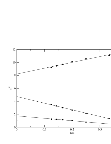
Figure 6: Plots of $m^{2}$ in units of $\frac{g^{\prime 2}}{\pi a^{2}}$ of low–energy non-cyclic bound states against $1/K$ with a linear fit to the data. The coupling $g^{\prime}\equiv g\sqrt{N_{c}}=1$. The circles correspond to bound state A, squares to the state B, diamonds to state C

Let us now discuss numerical results for the non-cyclic bound states. Again we follow bound states that we can easily identify from the properties of the bound states. In Fig. 6 we show $m^{2}$ of three low-energy states in units of $\frac{g^{\prime 2}}{\pi a^{2}}$ as a function of $1/K$ with $g^{\prime}\equiv g\sqrt{N_{c}}=1$. The state A denoted by circles is composed primarily of two bosons and two fermions, $b^{1{\dagger}}d^{1{\dagger}}a^{1{\dagger}}b^{1{\dagger}}$. The state B and C denoted by squares and diamonds are composed primarily of two fermions, $b^{1{\dagger}}b^{2{\dagger}}$ and $b^{1{\dagger}}b^{1{\dagger}}$, respectively. We show a linear fit to the data and see good conversion as $K\to\infty$ for all the three states. The extrapolated values for $m^{2}$ in the limit of $K\to\infty$ are given in Table 2. We also find the stringy states for the non-cyclic states.

	$b^{1{\dagger}}d^{1{\dagger}}a^{1{\dagger}}b^{1{\dagger}}$	$b^{1{\dagger}}b^{2{\dagger}}$	$b^{1{\dagger}}b^{1{\dagger}}$
$m^{2}_{\infty}$	1.764	4.744	8.204

Table 2: Extrapolated values for $m^{2}$ in units of $\frac{g^{\prime 2}}{\pi a^{2}}$ as $K\to\infty$ for State A, B, and C in Fig. 6 represented by its dominant Fock state.

Recall that we found in Sec. 4 that a bound state would be a linear combination of states of the four types we enumerated in Sec. 4. Hence, it is instructive to see if we can identify the three bound states with any of the four types. For $K=4$ we can identify all the three bound states with those that are killed by ${\cal Q}_{13}$ and whose mass in units of $\frac{g^{\prime 2}}{\pi a^{2}}$ are independent of $g^{\prime}$. However, as $K$ increases, we are not able to classify them into any particular type of the four. This is because as we increase $K$ the number of states becomes very large and the mass spectrum becomes dense. It is likely that these states mix with other nearby states with the same coupling dependence, giving rise to small changes in $m^{2}$ but still the same general coupling dependence. At this time however we are not able to resolve the spectrum in an enough detail to study these effects.

7 Discussion

We have presented the standard formulation of ${\cal N}$=1 SYM in 3+1 dimensions with a two spatial dimensional transverse lattice. Then we gave the SDLCQ formulation of the theory. We found that the standard formulation suffers from a fermion species doubling problem, while SDLCQ formulation does not. In the frame where the transverse momenta equal to zero, ${\cal N}$=1 SUSY in 3+1 dimensions is equivalent to ${\cal N}$=2 SUSY in 1+1 dimensions also known as ${\cal N}$=(2,2) SUSY. We were able to present $Q^{-}_{\alpha}$ which has the correct continuum form and yields by the SUSY algebra a discrete form of $P^{-}$, where $\alpha=1,2$. This $P^{-}$ then coincides with its continuum form in the continuum limit. Since $Q^{-}_{1}$ and $Q^{-}_{2}$ don’t commute with each other in our formulation, we are to use only one of them to solve the mass eigenvalue problem, preserving one exact SUSY.

We found that this $Q^{-}_{\alpha}$ consists of terms which are proportional to $g^{\prime}\equiv g\sqrt{N_{c}}$ and terms which go like $g^{\prime 3}$. This led us to investigate in some detail the $g^{\prime}$ dependence of the mass spectrum. From a simple toy model we concluded that the rich, complicated behavior of the mass spectrum with varying $g^{\prime}$ is due to some non-trivial coupling dependence of the wavefunctions. This is also responsible for a “transition” in the structure of a bound state when going from weak coupling to strong coupling. Because the dominant structure of a bound state changes with changing $g^{\prime}$.

We classified the bound states into two types, the cyclic and non-cyclic as we did in Ref. [13]. The cyclic bound states are those whose color flux goes all the way around in one or two of the transverse directions. The bound states whose color flux is localized and does not wind around are referred to as the non-cyclic bound states. For each type of the bound states, we were able to identify some bound states in the mass spectrum for $g^{\prime}=1$ and found the $K\to\infty$ limit of $m^{2}$.

For the cyclic bound states we were able to present $m^{2}$ as a function of the winding number $W_{I}$ in the $x_{I}$ direction with $I=1,2$. We found two very good fits to the data. The first fit $b+cW_{I}^{2}+d/W_{I}^{2}$ is motivated by the string theory, where the energy has the form $E=p2\pi/L+qTL$, where $p,q$ are some integers, $T$ is the string tension and $L$ is the period of the transverse lattice. The other fit $b+c/W_{I}+d/W_{I}^{2}$ is motivated by the operator structure of $Q^{-}_{\alpha}$. It appeared that $b+cW_{I}^{2}+d/W_{I}^{2}$ is preferable,

For the non-cyclic states as $1/K\to 0$ we saw good linear conversion of $m^{2}$ of the low-energy bound states that we could identify and gave the extrapolated values for $m^{2}$. We could identify for $K=4$ the bound states with a state whose $m^{2}$ in units of $\frac{g^{\prime 2}}{\pi a^{2}}$ are independent of $g^{\prime}$ though we were not able to do so for higher $K$’s because of the dense, and complicated spectrum.

In summary, we were able to present a formulation of SYM in 3+1 dimensions with one exact SUSY on a two dimensional transverse lattice and find the mass spectrum nonperturbatively. There remain however a number of important questions to answer. First and foremost it is of great importance to determine the form of $m^{2}$ numerically to better precision. It is interesting to see what the winding number dependence of $m^{2}$ is if both of the winding numbers are non-zero. We need to invent a method to resolve the dense spectrum at strong couplings. This will help us see if there is any “transition” in the form of $m^{2}$ as one goes from weak coupling to strong coupling. However, perhaps most importantly, as discussed in appendix A we need to know to what extent we’ve resolved the problem caused by the linearization of the link variables that we needed to quantize the fields. Knowing this tells us how reliable our numerical results are. Because one of our major simplifications in numerical calculation in the large $N_{c}$ limit comes about from the reduction of the transverse degrees of freedom whose justification relies upon the presence of the quantized fields and the vacuum. Restoration of SUSY for massive bound states, which has been broken by the linearlization gives us some confidence that our formulation indeed provides some sensible results. However, we would still have to clarify the issue to be more certain and confident. To this end, we need to compare our numerical results with some well-established theoretical predictions and with other numerical results obtained from the usual lattice calculation. Hence, it is of importance to apply our formulation to some other supersymmetric theories in higher than 1+1 dimensions, for instance, Wess-Zumino model, lattice sigma model, and SQED. It appears that the application is relatively straightforward. From more practical point of view, a next question to ask is what happens if one includes scalars and their superpartners in theory. We did not consider this case in this paper simply because this was the first attempt to formulate SYM in 3+1 dimensions with one exact SUSY on a two dimensional transverse lattice and, thus, we wanted to consider the simplest possible case. However, it is of great interest to consider the question in the future. The authors believe that when we are able to answer all those questions, we will also be able to test the predictions made by Armoni, Shifman and Veneziano [3, 4].

Appendix A Eguchi-Kawai Reduction

For our numerical calculation we’ve set $N_{sites}=1$, in other words, we’ve dropped the site indices. This reduction of the transverse degrees of freedom has brought a great amount of simplification in our calculation and needs some detailed justification. Since it is only the supercharges that we need to do our calculation, if the supercharges do not depend on the site indices in the large $N_{c}$ limit, neither does any quantity that can be computed from $Q^{-}_{\alpha}$, for instance $m^{2}$ for our case. Therefore, in order to justify the reduction of the degrees of freedom for our purposes, it suffices to show the independence of $Q^{-}_{\alpha}$ of the site indices in the large $N_{c}$ limit. In this appendix, in particular, we will show that in the large $N_{c}$ limit the leading order terms of the supercharges $Q^{-}_{\alpha}$ with keeping all the site indices are the same as those with setting $N_{sites}=1$. We should note that this sort of arguments about the justification of the reduction on a transverse lattice have already been given in literature, for instance see Refs. [16, 23, 24] and our arguments below closely parallel those in the Refs. [16, 24].

In what follows we only consider $Q^{-}_{1}$, however the same arguments apply equally well to $Q^{-}_{2}$. For definiteness let us first consider a Fock state denoted by

$$\sum_{n}{\rm tr}[\ldots d^{1{\dagger}}_{n}(k_{1})a^{1{\dagger}}_{n}(k_{2})b^{1{\dagger}}_{n}(k_{3})a^{1{\dagger}}_{n-i_{1}}(k_{4})\ldots]|0\rangle,$$

where we’ve written $k^{+}\equiv k$, $n\equiv(i,j)$ is the transverse lattice site, $i_{1}$ is the vector of length $a$ pointing the $x^{1}$ direction, $a$ is the lattice spacing, and the dots represent some creation operators. When we act on this state with $Q^{-}_{1}$, we get for example from one of the terms in $Q^{-}_{1}$, say $b^{2{\dagger}}d^{1}a^{1}\equiv\sum_{n}{\rm tr}[b^{2{\dagger}}_{n}(p_{1}+p_{2})d^{1}_{n}(p_{1})a^{1}_{n}(p_{2})]$ on it

$$N_{c}\sum_{n}{\rm tr}[\ldots b^{2{\dagger}}_{n}(k_{1}+k_{2})b^{1{\dagger}}_{n}(k_{3})a^{1{\dagger}}_{n-i_{1}}(k_{4})\ldots]|0\rangle.$$

If we set $N_{sites}=1$, then the Fock state now becomes

$${\rm tr}[\ldots d^{1{\dagger}}(k_{1})a^{1{\dagger}}(k_{2})b^{1{\dagger}}(k_{3})a^{1{\dagger}}(k_{4})\ldots]|0\rangle,$$

and upon the action of $Q^{-}_{1}$ we get from $b^{2{\dagger}}d^{1}a^{1}\equiv{\rm tr}[b^{2{\dagger}}(p_{1}+p_{2})d^{1}(p_{1})a^{1}(p_{2})]$ on it

$$N_{c}{\rm tr}[\ldots b^{2{\dagger}}(k_{1}+k_{2})b^{1{\dagger}}(k_{3})a^{1{\dagger}}(k_{4})\ldots]|0\rangle,$$ (19)

and one more term

$${\rm tr}[\ldots b^{2{\dagger}}(k_{1}+k_{4})\ldots]{\rm tr}[a^{1{\dagger}}(k_{2})b^{1{\dagger}}(k_{3})]|0\rangle.$$ (20)

Notice that the extra term Eq. (20) we get by setting $N_{sites}=1$ is down by $1/N_{c}$ compared to the leading order term Eq. (19) and thus we can ignore it in the large $N_{c}$ limit. Of course, in the above example, we could and would have gotten many more terms depending on what we have in those ’dots’ inside the trace of the Fock state we considered. However, it is easy to see that our conclusion remains the same; all the extra terms we get by having only one site are down by $1/N_{c}$ or more powers of $1/N_{c}$. This all comes down to the fact that we can have only single-traced states in the large $N_{c}$ limit. Therefore, we find that the leading order terms of $Q^{-}_{\alpha}$ are the same whether we keep track of the site indices or not. Although this proof is for finite $K$, we suspect that the same result would persist at infinite $K$.

The way to justify the reduction here should be contrasted to the way exploited by Eguchi and Kawai [18]. Eguchi and Kawai showed that in the large $N_{c}$ limit we can work with only one lattice site in each of the space-time directions in Euclidean space. However, the proof was based on, among others, the assumption that $U(1)^{d}$ symmetry is not spontaneously broken, where $d$ is the number of the space-time dimensions. This assumption was found to be wrong for $d>2$ at weak couplings by the authors of Ref.[19]. To resolve this problem, there have been many models proposed, for instance quenching [19] and twisted [20] lattice formulations. Here in our formulation, however, we believe that we do not have to introduce any of the modified lattice formulation since the way we justify the reduction is quite different the way Eguchi and Kawai do. Our proof stands on its own feet regardless of us maintaining the $U(1)^{d}$ symmetry or not and, therefore, would not suffer from the problem associated with the naive Eguchi-Kawai reduction as we go from weak to strong couplings.

A question, however, remains. That is the question of how well we’ve managed to quantize the fields since all our arguments above rely on the fact that we have the quantized fields and true vacuum. Put in another way, how good the reduction procedure is depends on how good our quantization procedure is. Recall that to quantize, we had to “linearize” the unitary link variables, which leads to the breakdown of SUSY. The authors of Refs. [16, 23, 24] make use of the “color-dielectric” formulation to resolve the problem for non-supersymmetric theories. Although this formulation resolves the problem completely, it prevents one from going to small lattice spacings. In our formulation we do not have that constraint on the lattice spacing. However, the price we pay is that we resolve the problem of the linearization partially, not completely. Thus, it is of great importance for one to see to what extent we’ve resolved the problem and, if possible and necessary, to find a way to get around it completely. Up to this point we are not able to answer this question, but this is one of the crucial steps we should take towards a more sensible supersymmetric model on a lattice within our formulation.

Appendix B ${\cal N}$=1 super-algebra in Majorana representation

In this appendix we give the super-algebra in Majorana representation in $D+1$ dimensional light-cone coordinates where $D=1,2,3$.

In Majorana representation Majorana spinors have real component fields, and can be written as

$$\Psi_{M}=\left(\begin{array}[]{c}\theta_{L}\\ \theta_{R}\end{array}\right),$$

where $\theta_{L}$, $\theta_{R}$ are left-moving, right-moving spinors with real components. This implies that the supercharge $Q$ is also a Majorana spinor with real components of the form

$$Q=\int d^{D}xj^{+}=\left(\begin{array}[]{c}Q_{L}\\ Q_{R}\end{array}\right)\equiv\left(\begin{array}[]{c}Q^{+}\\ Q^{-}\end{array}\right),$$

where the integration is taken over the $D$ spatial dimensions, $j^{\mu}$ is the supercurrent, which is a Majorana spinor.

In terms of the Majorana super-charge, the super-algebra is given by

$$\{Q,\bar{Q}\}=2\Gamma^{\mu}P_{\mu},$$ (21)

where $\bar{Q}\equiv Q^{{\dagger}}\Gamma^{0}$ in any representation, and thus $\bar{Q}=Q^{T}\Gamma^{0}$ in Majorana representation.

B.1 D=1

For 1+1 dimensional case, we have $\Gamma^{0}=\sigma^{2}$ and $\Gamma^{1}=i\sigma^{1}$, so that

$$\Gamma^{+}\equiv\frac{\Gamma^{0}+\Gamma^{1}}{\sqrt{2}}=i\left(\begin{array}[]{cc}0&0\\ \sqrt{2}&0\end{array}\right),\qquad\Gamma^{-}\equiv\frac{\Gamma^{0}-\Gamma^{1}}{\sqrt{2}}=i\left(\begin{array}[]{cc}0&-\sqrt{2}\\ 0&0\end{array}\right)$$

and $\bar{Q}=i(Q^{-},-Q^{+})$. Thus, Eq. (21) reads

$$\{Q,\bar{Q}\}=2\Gamma^{\mu}P_{\mu}=i\left(\begin{array}[]{cc}0&-2\sqrt{2}P_{-}\\ 2\sqrt{2}P_{+}&0\end{array}\right)=i\left(\begin{array}[]{cc}0&-2\sqrt{2}P^{+}\\ 2\sqrt{2}P^{-}&0\end{array}\right),$$

or

$$\{Q^{\pm},Q^{\pm}\}=2\sqrt{2}P^{\pm},\quad\{Q^{+},Q^{-}\}=0.$$

B.2 D=2

In this case $\Gamma^{0}=\sigma^{2}$, $\Gamma^{1}=i\sigma^{1}$ and $\Gamma^{2}=\Gamma^{\perp}=i\sigma^{3}$. Therefore,

$$\{Q,\bar{Q}\}=2\Gamma^{\mu}P_{\mu}=i\left(\begin{array}[]{cc}2P_{\perp}&-2\sqrt{2}P_{-}\\ 2\sqrt{2}P_{+}&-2P_{\perp}\end{array}\right)=i\left(\begin{array}[]{cc}-2P^{\perp}&-2\sqrt{2}P^{+}\\ 2\sqrt{2}P^{-}&2P^{\perp}\end{array}\right),$$

or

$$\{Q^{\pm},Q^{\pm}\}=2\sqrt{2}P^{\pm},\quad\{Q^{+},Q^{-}\}=-2P^{\perp}.$$

B.3 D=3

In 3+1 dimensions Majorana spinors have four components and thus the supercharge can be written as

$$Q=\left(\begin{array}[]{c}Q^{+}\\ Q^{-}\end{array}\right)\equiv\left(\begin{array}[]{c}Q^{+}_{1}\\ Q^{+}_{2}\\ Q^{-}_{1}\\ Q^{-}_{2}\end{array}\right),\quad\bar{Q}=Q^{T}\Gamma^{0}=i(Q^{-}_{2},-Q^{-}_{1},Q^{+}_{2},-Q^{+}_{1}).$$

Gamma matrices are $4\times 4$ matrices given by

$$\Gamma^{0}\equiv\left(\begin{array}[]{cc}0&\sigma_{2}\\ \sigma_{2}&0\end{array}\right),\quad\Gamma^{1}\equiv i\left(\begin{array}[]{cc}\sigma_{1}&0\\ 0&\sigma_{1}\end{array}\right),\quad\Gamma^{2}\equiv i\left(\begin{array}[]{cc}\sigma_{3}&0\\ 0&\sigma_{3}\end{array}\right),\quad\Gamma^{3}\equiv\left(\begin{array}[]{cc}0&-\sigma_{2}\\ \sigma_{2}&0\end{array}\right),$$

$$\Gamma^{+}\equiv\frac{\Gamma^{0}+\Gamma^{3}}{\sqrt{2}}=\left(\begin{array}[]{cc}0&0\\ \sqrt{2}\sigma_{2}&0\end{array}\right),\quad\Gamma^{-}\equiv\frac{\Gamma^{0}-\Gamma^{3}}{\sqrt{2}}=\left(\begin{array}[]{cc}0&\sqrt{2}\sigma_{2}\\ 0&0\end{array}\right).$$

Then Eq. (21) yields

$$\{Q,\bar{Q}\}=2\Gamma^{\mu}P_{\mu}=2\left(\begin{array}[]{cc}i\sigma^{1}P_{1}+i\sigma^{3}P_{2}&\sqrt{2}\sigma^{2}P_{-}\\ \sqrt{2}\sigma^{2}P_{+}&i\sigma^{1}P_{1}+i\sigma^{3}P_{2}\end{array}\right)$$

$$=2i\left(\begin{array}[]{cccc}-P^{2}&-P^{1}&0&-\sqrt{2}P^{+}\\ -P^{1}&P^{2}&\sqrt{2}P^{+}&0\\ 0&-\sqrt{2}P^{-}&-P^{2}&-P^{1}\\ \sqrt{2}P^{-}&0&-P^{1}&P^{2}\end{array}\right).$$

Hence, we find

$$\{Q^{\pm}_{\alpha},Q^{\pm}_{\beta}\}=2\sqrt{2}P^{\pm}\delta_{\alpha\beta},$$

$$\{Q^{+}_{1},Q^{-}_{1}\}=-\{Q^{+}_{2},Q^{-}_{2}\}=2P^{1},\quad\{Q^{+}_{1},Q^{-}_{2}\}=\{Q^{+}_{2},Q^{-}_{1}\}=-2P^{2},$$

where $\alpha,\beta=1,2$. Note that if $P^{1}=P^{2}=0$, then this algebra coincides with the one for ${\cal N}$=2 SUSY in 1+1 dimensions also known as ${\cal N}$=(2,2) SUSY.

References

- [1] J. M. Maldacena, Adv. Theor. Math. Phys. 2, 231 (1998) [Int. J. Theor. Phys. 38, 1113 (1999)] [arXiv:hep-th/9711200].
- [2] S. Kachru and E. Silverstein, Phys. Rev. Lett. 80, 4855 (1998) [arXiv:hep-th/9802183]; A. E. Lawrence, N. Nekrasov and C. Vafa, Nucl. Phys. B 533, 199 (1998) [arXiv:hep-th/9803015]; M. Schmaltz, Phys. Rev. D 59, 105018 (1999) [arXiv:hep-th/9805218].
- [3] A. Armoni, M. Shifman and G. Veneziano, Nucl. Phys. B 667, 170 (2003) [arXiv:hep-th/0302163].
- [4] A. Armoni, M. Shifman and G. Veneziano, Phys. Rev. Lett. 91, 191601 (2003) [arXiv:hep-th/0307097].
- [5] A. G. Cohen, D. B. Kaplan, E. Katz and M. Unsal, JHEP 0308, 024 (2003) [arXiv:hep-lat/0302017]; JHEP 0312, 031 (2003) [arXiv:hep-lat/0307012];
- [6] F. Sugino, JHEP 0401, 015 (2004) [arXiv:hep-lat/0311021]; JHEP 0403, 067 (2004) [arXiv:hep-lat/0401017].
- [7] F. Sugino, arXiv:hep-lat/0409036; arXiv:hep-lat/0410035.
- [8] J. Giedt, Nucl. Phys. B 668, 138 (2003) [arXiv:hep-lat/0304006]; Nucl. Phys. B 674, 259 (2003) [arXiv:hep-lat/0307024]; arXiv:hep-lat/0405021.
- [9] S. Catterall, JHEP 0305, 038 (2003) [arXiv:hep-lat/0301028].
- [10] S. Catterall, arXiv:hep-lat/0410052.
- [11] W. Bietenholz, Mod. Phys. Lett. A 14, 51 (1999) [arXiv:hep-lat/9807010]; Y. Kikukawa and Y. Nakayama, Phys. Rev. D 66, 094508 (2002) [arXiv:hep-lat/0207013]; K. Itoh, M. Kato, H. Sawanaka, H. So and N. Ukita, JHEP 0302, 033 (2003) [arXiv:hep-lat/0210049]; S. Catterall and S. Karamov, Phys. Rev. D 68, 014503 (2003) [arXiv:hep-lat/0305002]; S. Catterall and S. Ghadab, JHEP 0405, 044 (2004) [arXiv:hep-lat/0311042]; A. D’Adda, I. Kanamori, N. Kawamoto and K. Nagata, arXiv:hep-lat/0406029; J. Giedt and E. Poppitz, arXiv:hep-th/0407135; J. Giedt, R. Koniuk, E. Poppitz and T. Yavin, arXiv:hep-lat/0410041.
- [12] For a brief but inclusive review on this subject, see for example A. Feo, Nucl. Phys. Proc. Suppl. 119, 198 (2003) [arXiv:hep-lat/0210015]; arXiv:hep-lat/0410012.
- [13] M. Harada and S. Pinsky, Phys. Lett. B 567, 277 (2003) [arXiv:hep-lat/0303027].
- [14] N. Arkani-Hamed, A. G. Cohen, and H. Georgi, Phys. Rev. Lett.86, 4757 (2001) arXiv:hep-th/0104005; C. T. Hill, S. Pokorski and J. Wang, Phys. Rev. D 64, 105005 (2001) arXiv:hep-th/0104035.
- [15] W. A. Bardeen and R. B. Pearson, Phys. Rev. D14, 547 (1976) ;W. A. Bardeen, R. B. Pearson and E. Rabinovici, Phys. Rev. D 21, 1037 (1980).
- [16] M. Burkardt and S. Dalley, Prog. Part. Nucl. Phys. 48, 317 (2002) [arXiv:hep-ph/0112007].
- [17] Y. Matsumura, N. Sakai and T. Sakai, Phys. Rev. D 52, 2446 (1995) [arXiv:hep-th/9504150]; O. Lunin and S. Pinsky, AIP Conf. Proc. 494, 140 (1999), arXiv:hep-th/9910222.
- [18] T. Eguchi and H. Kawai, Phys. Rev. Lett. 48, 1063 (1982).
- [19] G. Bhanot, U. M. Heller and H. Neuberger, Phys. Lett. B 113, 47 (1982).
- [20] A. Gonzalez-Arroyo and M. Okawa, Phys. Rev. D 27, 2397 (1983); T. Eguchi and R. Nakayama, Phys. Lett. B 122, 59 (1983).
- [21] M. Burkardt and H. El-Khozondar, Phys. Rev. D 60, 054504 (1999) [arXiv:hep-ph/9805495];
- [22] M. Harada and S. Pinsky, Phys. Rev. D 70, 087701 (2004) [arXiv:hep-lat/0408026].
- [23] S. Dalley and B. van de Sande, Phys. Rev. D 59, 065008 (1999) [arXiv:hep-th/9806231]; M. Burkardt, AIP Conf. Proc. 494, 239 (1999) [arXiv:hep-th/9908195].
- [24] S. Dalley and B. van de Sande, Phys. Rev. D 56, 7917 (1997) [arXiv:hep-ph/9704408].
- [25] F. Antonuccio, O. Lunin, and S. S. Pinsky, Phys. Lett. B 429, 327 (1998), arXiv:hep-th/9803027; F. Antonuccio, O. Lunin, and S. Pinsky, Phys. Rev. D 58, 085009 (1998), arXiv:hep-th/9803170; F. Antonuccio, O. Lunin, S. Pinsky , and S. Tsujimaru, Phys. Rev. D 60, 115006 (1999), arXiv:hep-th/9811254.