Phase diagram of QCD at finite temperature and chemical potential from lattice simulations with dynamical Wilson quarks

Abstract

We present the first results for lattice QCD at finite temperature $T$ and chemical potential $\mu$ with four flavors of Wilson quarks. The calculations are performed using the imaginary chemical potential method at $\kappa=0$, 0.001, 0.15, 0.165, 0.17 and 0.25, where $\kappa$ is the hopping parameter, related to the bare quark mass $m$ and lattice spacing $a$ by $\kappa=1/(2ma+8)$. Such a method allows us to do large scale Monte Carlo simulations at imaginary chemical potential $\mu=i\mu_{I}$. By analytic continuation of the data with $\mu_{I}<\pi T/3$ to real values of the chemical potential, we expect at each $\kappa\in[0,\kappa_{chiral}]$, a phase transition line on the $(\mu,T)$ plane, in a region relevant to the search for quark gluon plasma in heavy-ion collision experiments. The transition is first order at small or large quark mass, and becomes a crossover at intermediate quark mass.

I Introduction

QCD predicts a transition between hadronic matter (quark confinement) to quark-gluon plasma (quark deconfinement) at sufficient high temperature $T$ and small chemical $\mu$. This matter might have existed in early universe immediately after the big bang. The main purpose of heavy-ion collision experiments at LHC (CERN), SPS, and RHIC (BNL) is to recreate such an environment. At large $\mu$ and lower $T$, several QCD-inspired models predict the existence of a color-superconductivity phase, which might be relevant to neutron star or quark star physics. Therefore, it is of great significance to study the QCD phase structure at larger $\mu$. Because QCD is still strongly coupled at criticality, perturbative methods do not apply. Lattice gauge theory (LGT) is the most reliable tool for investigating the phase transition from first principles.

In the continuum, the thermodynamics is described by the grand partition function

$$Z(\mu,T)={\rm Tr}~{}e^{-\left(\hat{H}-\mu\hat{N_{q}}\right)/T},$$ (1)

where $\hat{H}$ is the Hamiltonian, $\mu$ is the chemical potential, and $\hat{N_{q}}=\int d^{3}x{\bar{\psi}}\psi$ is the quark number operator.

In the Lagrangian formulation of SU(3), LGT at finite $\mu$, the effective fermionic action is complex and traditional Monte Carlo (MC) techniques with importance sampling do not work. The recent years have seen enormous effortsMuroya:2003qs ; Katz:2003up ; Lombardo:2004uy on solving the complex action problem, and some very interesting informationFodor:2002hs on the phase diagram for QCD with Kogut-Susskind (KS) fermions at large $T$ and small $\mu$ has been obtained. The KS approach to lattice fermions thins the fermionic degrees of freedom in naive fermions, but it does not completely solve the species doubling problem. It preserves the partial chiral symmetry, but it breaks the flavor symmetry. One staggered flavor corresponds to four flavors in reality and the fermionic determinant is replaced by the fourth root. Such a replacement is mathematically un-provenNeuberger:2004be and it might lead to the locality problem in numerical simulationsBunk:2004br .

Wilson’s approach to lattice fermionsWilson:1974sk avoids the species doubling and preserves the flavor symmetry, but it explicitly breaks the chiral symmetry, one of the most important symmetries of the original theory. Non-perturbative fine-tuning of the bare fermion mass has to be done, in order to define the chiral limit. There have been some MC simulations of LGT with Wilson fermions at finite temperature, but no numerical investigation at finite chemical potential. In Ref. Luo:2004mc , the QCD phase structure on the $(\mu,T)$ plane was investigated using Hamiltonian lattice QCD with Wilson fermions at strong coupling. For $N_{f}/N_{c}<1$, with $N_{c}=3$ being the number of colors and $N_{f}$ being the number of flavors, a tricritical point is found, separating the first order and second order chiral phase transitions.

Neuberger’s overlap fermion approachNeuberger:1997fp solves the species doubling problem and preserves the chiral symmetry and flavor symmetry, by introducing exponentially decaying non-local terms in the action. However, the computational costsFodor:2003bh for dynamical overlap fermions are typically two orders of magnitude heavier than for the Wilson or KS formulations. This is certainly beyond the current computer capacity.

In this paper, we perform the first MC simulations of Lagrangian LGT with four flavors of dynamical Wilson quarks at finite temperature and imaginary chemical potential $i\mu_{I}$, and study the phase structure in the $(\mu,T,\kappa)$ space, by analytical continuation to the real chemical potential.

II LATTICE FORMULATION

The basic idea of lattice gauge theoryWilson:1974sk , as proposed by K. Wilson in 1974, is to replace continuous space-time by a discrete grid with lattice spacing $a$. Gluons live on links $U_{j}(x)=e^{-ig\int_{x}^{x+\hat{j}a}dx^{\prime}A_{j}(x^{\prime})}$, and quarks live on lattice sites. The continuum Yang-Mills action $S_{g}=\int d^{4}x~{}{\rm Tr}~{}F_{jl}(x)F_{jl}(x)/2$ is replaced by

$$S_{g}=-{\beta\over 6}\sum_{p}{\rm Tr}(U_{p}+U_{p}^{\dagger}-2),$$ (2)

where $\beta=6/g^{2}$, and $U_{p}$ is the ordered product of link variables $U$ around an elementary plaquette. The continuum quark action $S_{f}=\int d^{4}x~{}\bar{\psi}^{cont}(x)(\gamma_{j}D_{j}+m)\psi^{cont}(x)$ is replaced by

$$S_{f} = \sum_{x,y}{\bar{\psi}}(x)M_{x,y}\psi(y).$$ (3)

For Wilson fermions, the quark field $\psi$ on the lattice is related to the continuum one $\psi^{cont}$ by $\psi=\psi^{cont}\sqrt{a^{3}/(2\kappa)}$ with $\kappa=1/(2ma+8)$ the hopping parameter. $M$ is the fermionic matrix:

$$M_{x,y}=\delta_{x,y} - \kappa\sum_{j=1}^{4}\bigg{[}(1-\gamma_{j})U_{j}(x)\delta_{x,y-\hat{j}}$$ (4)

$$+ (1+\gamma_{j})U_{j}^{\dagger}(x-\hat{j})\delta_{x,y+\hat{j}}\bigg{]}.$$

If we consider $N_{f}$ degenerate flavors of quarks, the partition function is

$$Z = \int[dU][d\bar{\psi}][d\psi]e^{-S_{g}-S_{f}}$$ (5)

$$= \int[dU]\left({\rm Det}M[U]\right)^{N_{f}}e^{-S_{g}}.$$

In the Lagrangian formulation of LGT, following Ref. Hasenfratz:1983ba , the chemical potential is introduced by replacing the link variables in the temporal direction in fermion action with:

$$U_{4}(x)\rightarrow e^{a\mu}U_{4}(x),~{}~{}U^{{\dagger}}_{4}(x)\rightarrow e^{-a\mu}U^{{\dagger}}_{4}(x).$$ (6)

The fermionic action is reduced to the continuum one when $a\to 0$. However, the effective fermionic action in the partition function becomes complex, and forbids MC simulation with importance sampling. Several revised methods, e.g., improved reweightingFodor:2001au and imaginary chemical potentialLombardo:1999cz ; Azcoiti:2004ri methods, were proposed to simulate QCD with KS fermions at finite $\mu$.

Lattice QCD at imaginary chemical potential does not suffer the complex action problem. In this paper, we will apply this method to the MC study of the phase structure of Wilson fermions. We will measure the expectation of the Polyakov loop, chiral condensate and their susceptibilities.

The Polyakov loop (Wilson line) is defined as

$$P(\vec{x})={\rm Tr}\left[\prod_{t=0}^{N_{t}-1}{U_{4}(\vec{x},t)}\right],$$ (7)

where $N_{t}$ is the number of lattice sites in the temporal direction. $P(\vec{x})$ is used to scale the interaction strength between quarks. In pure gauge theory, non-zero $P(\vec{x})$ is a signal of quark deconfinement. In practice, we measure its expectation value over configurations generated in MC simulations with the probability distribution $\left({\rm Det}M[U]\right)^{N_{f}}e^{-S_{g}}/Z$.

The chiral condensate is defined as

$$\langle\bar{\psi}\psi\rangle = \frac{1}{Z}\int[dU][d\bar{\psi}][d\psi]\bar{\psi}\psi e^{-S_{g}-S_{f}}$$

$$= {1\over ZVN_{t}}\int[dU]{\rm Tr}\left(M^{-1}[U]\right)\left({\rm Det}M[U]\right)^{N_{f}}e^{-S_{g}},$$

where $V$ is the spatial lattice volume. With suitable subtraction, it serves as the order parameter of chiral-symmetry breaking in the non-perturbatively defined chiral limit, $\kappa=\kappa_{chiral}$ where the pion is massless.

Strictly speaking, if the dynamical quarks play a role, $P(\vec{x})$ is no longer an order parameter for deconfinement; $\langle\bar{\psi}\psi\rangle$ is no longer an order parameter for spontaneous chiral-symmetry breaking, if $\kappa\neq\kappa_{chiral}$. However, when the system is at criticality, in particular for the first order transition, one should observe sharp changes in these quantities. Of course, this method is very rough. At the transition point, there will be a peak in the susceptibility, because the fluctuation of physical quantities is very strong. Therefore, the susceptibility will provide more useful information about the transition. The susceptibility of a quantity

$$O=\frac{1}{VN_{t}}\sum_{x,t}O(x)$$ (9)

is defined as

$$\chi=VN_{t}\langle(O^{2}-\langle O\rangle^{2})\rangle.$$ (10)

At criticality, the maximum value of $\chi$ behaves as $\chi_{max}\propto V^{\alpha}$, with $\alpha$ the critical exponent. If $\alpha=0$, the transition is just a crossover; If $0<\alpha<1$, it is a second order phase transition; If $\alpha=1$, it is a first order phase transition, accompanying the double peak structure in the histogram of the quantity $O$ and flip-flops between the two states in the MC history.

III PHASE DIAGRAM ON THE $(\mu_{I},T)$ PLANE

Many years ago, Roberge and Weiss (RW)Roberge:1986mm made the first analytical study of the phase structure of a gauge theory with fermions. Replacing $\mu$ by $i\mu_{I}$ ($\mu_{I}$ being a real number) and introducing $\theta=\mu_{I}/T$, the grand partition function (1) has the behavior Roberge:1986mm

$$Z(\theta)=Z(\theta+2\pi).$$ (11)

If the gauge group is SU$(N_{c})$, the exact period is $2\pi/N_{c}$. It implies the theory has a $Z_{3}$ symmetry for $N_{c}=3$, which is clearly an artifact of imaginary $\mu$ and unphysical.

Figure 1: Schematic phase diagram of QCD on the $(\mu_{I},T)$ plane, suggested by Roberge and Weiss. For $T\geq T_{E}$, there are first order phase transitions at $a\mu_{I}=2\pi(k+1/2)/N$, characterized by discontinuity in the Polyakov loop. Here $N=N_{c}N_{t}$ and $N_{t}a=1/T$. [There is no phase transition across the dashed lines; they just illustrate the location of $T_{E}$ or $a\mu_{I}=2\pi(k+1/2)/N$].

Figure 2: Schematic phase diagram of QCD on the $(\mu_{I},T)$ plane, suggested by lattice MC study.

Figure 1 shows the phase diagram of QCD at imaginary chemical potential, suggested by Roberge and WeissRoberge:1986mm . Below some $T_{E}$, there is no phase transition. Above $T_{E}$ and at $\theta=2\pi(k+1/2)/N_{c}$, with $k=0,1,2,...$, there are first order RW phase transitions between different $Z_{3}$ sectors, characterized by the appearance of discontinuity in the Polyakov loop. However, later MC simulations with KS fermionsdeForcrand:2002ci ; D'Elia:2002gd suggest a phase diagram as shown in Fig. 2, i.e., there are additional chiral/deconfinement transition lines for $T_{C}\leq T\leq T_{E}$, with $T_{C}$ being the critical temperature at $\mu=0$. However, only the critical line lies within $\theta\in[0,\pi/N_{c})$ and $T\in[T_{C},T_{E})$ is relevant for the analytical continuation to the real chemical potential in the physical case. I.e., the imaginary chemical potential method works only for $\mu_{I}/T<\pi/N_{c}$.

IV MC SIMULATIONS

In this section, we will present the first results for QCD with four flavors of Wilson fermions at finite $T$ and $i\mu_{I}$.

The $R$ algorithmGottlieb:1987mq was used. We modified the MILC collaboration’s public LGT codeMilc to simulate the case of imaginary chemical potential. The simulations were done at lattice size $V\times N_{t}=8^{3}\times 4$ and hopping parameter $\kappa=$0, 0.001, 0.15, 0.165 0.17, and 0.25. At some $a\mu_{I}$, $\beta$ and $\kappa$ values, finite size scaling analysis was performed on different lattices. There are 20 molecular steps with size $\delta\tau=0.02$ for each configuration. For each $\beta$ and $a\mu_{I}$, we generated at least 20,000 configurations, after 4000 warmups. 20 iterations are carried out between measurements. Around the area where the thermodynamical observables change rapidly, we raised the statistics at least two times. All simulations were done on our PC clusters. The cluster with 20 Pentium III-500 CPUsLuo:2000iz ; Luo:2002kr was built in 2000, and has been upgraded to 60 CPUs, with 40 new AMD Opteron-242 CPUs.

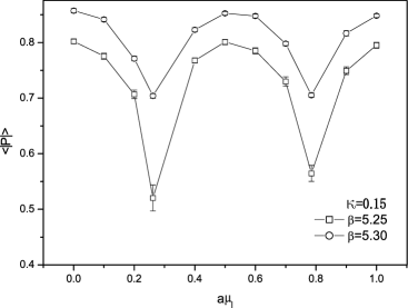
Figure 3: Polyakov loop norm as a function of $a\mu_{I}$ at $\kappa=0.15$ and two different $\beta$.

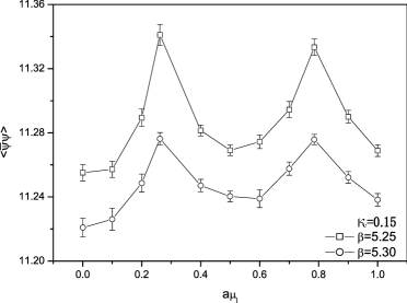
Figure 4: Chiral condensate as a function of $a\mu_{I}$ at $\kappa=0.15$ and two different $\beta$.

We have more complete data at $\kappa=0.15$ than other $\kappa$ values. Figure 3 plots the results for the Polyakov loop norm $\langle|P({\vec{x}})|\rangle$ as a function of $a\mu_{I}$ at two different and larger values of $\beta$ (corresponding to higher $T$). The data for $\langle\bar{\psi}\psi\rangle$ are shown in Fig. 4. As one sees, these quantities are approximately periodic with period $\pi/6$, confirming the RW period for $a\mu_{I}$ to be $2\pi aT/3=2\pi/(3N_{t})$. Furthermore, at $a\mu_{I}=2(k+1/2)\pi/(3N_{t})$, $k=0,1,...$, there is a rapid change in the thermodynamical quantities, indicating the RW phase transition at higher $T$ (larger $\beta$). Figure 5 is a more detailed scan for the phase of the Polyakov loop at $\beta=5.25$. At $a\mu_{I}=0.26$, it changes rapidly. Figure 6 plots the MC history of the phase of the Polyakov loop. There is a clear signal for first order phase transition at $a\mu_{I}=0.26$, confirming the existence of RW transition between different $Z_{3}$ sectors at $a\mu_{I}=\pi/(3N_{t})=\pi/12$.

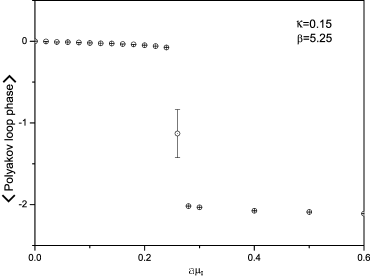
Figure 5: Phase of the Polyakov loop as a function of $a\mu_{I}$ at $\beta=5.25$ and $\kappa=0.15$.

Figure 6: MC history of the phase of the Polyakov loop at $a\mu_{I}=0.26$, $\beta=5.25$, and $\kappa=0.15$.

To locate the chiral/deconfinement phase transition line, we made more detailed measurements of $\langle|P({\vec{x}})|\rangle$, $\chi_{|P|}$, $\langle\bar{\psi}\psi\rangle$, and $\chi_{\bar{\psi}\psi}$ for $a\mu_{I}<\pi/(3N_{t})$.

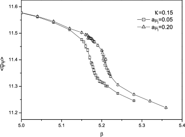
Figure 7: Chiral condensate as a function of $\beta$ at $\kappa=0.15$ and two different values of $a\mu_{I}$.

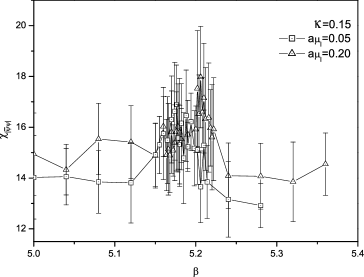
Figure 8: Chiral susceptibility as a function of $\beta$ at $\kappa=0.15$ and two different values of $a\mu_{I}$.

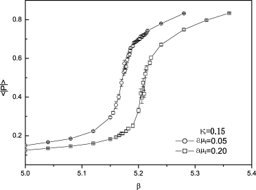
Figure 9: Polyakov loop norm as a function of $\beta$ at $\kappa=0.15$ and two different $a\mu_{I}$.

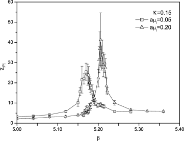
Figure 10: Susceptibility of the Polyakov loop norm as a function of $\beta$ at $\kappa=0.15$ and two different $a\mu_{I}$.

Figures 7 and 8 show respectively $\langle\bar{\psi}\psi\rangle$ and $\chi_{\bar{\psi}\psi}$ versus $\beta$ at $a\mu_{I}=0.05$ and 0.20 for $\kappa=0.15$; Figures 9 and 10 show the results for $\langle|P|\rangle$ and $\chi_{|P|}$. In the rapid changing area, the Polyakov loop and its susceptibility behave more singularly than the chiral condensate and chiral susceptibility. From the position of the peak in the susceptibilities, we determine the transition point. A collection of transition points $(a\mu_{I},\beta_{C})$ is listed in Tab. 1. In Refs. deForcrand:2002ci ; D'Elia:2002gd , it has generally been argued that for small $a\mu_{I}$, the transition line $\beta_{C}(a\mu_{I})$ can be expressed as a Taylor series with even power of $a\mu_{I}$. Due to limited data, the series is truncated to the quadratic term. We use the least squares method to fit the data in Tab. 1 for $\kappa=0.15$, and obtain an equation for the transition line:

$$\beta_{C}=5.169(9)+0.954(33)\left(a\mu_{I}\right)^{2}+O\left(a^{4}\mu_{I}^{4}\right),$$ (12)

with error bars coming from the fit.

$a\mu_{I}$		$\beta_{C}$
0.00		5.168(2)
0.05		5.170(2)
0.10		5.180(2)
0.14		5.187(2)
0.18		5.200(2)
0.20		5.206(2)
0.22		5.217(2)

Table 1: Collection of transition points for $\kappa=0.15$, determined by locating the peak of the susceptibilities, with error bars coming from the scan precision.

Nevertheless, at this $\kappa$, there is no obvious double peak structure in the histograms of thermodynamical observables. To determine the nature of the transition, one has to do a finite size study. Let us take the transition point at $a\mu_{I}=0.14$ and $\beta=5.187$ in Tab. 1 as an example. Figure 11 compares $\chi_{|P|}$ for spacial volumes $V=L^{3}=8^{3}$ and $12^{3}$ around the transition point (with $\Delta\beta=0.002$). Within error bars, the locations and heights of the peaks are consistent. At this $\beta$, we did the longest simulations on $8^{3}\times 4$, $10^{3}\times 4$, $12^{3}\times 4$, $14^{3}\times 4$, and $16^{3}\times 4$ lattices, with statistics at least four times higher than other non-transition points. As shown in Fig. 12, $\chi_{|P|}$ does not increase as $L$. This implies that the transition point at $a\mu_{I}=0.14$ and $\beta=5.187$ for $\kappa=0.15$ is just a crossover.

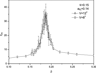
Figure 11: Susceptibility of the Polyakov loop norm as a function of $\beta$ at $a\mu_{I}=0.14$ and $\kappa=0.15$ for different spatial volumes $V=8^{3}$ and $12^{3}$.

Figure 12: Susceptibility of the Polyakov loop norm as a function of the spacial extent $L$ at $a\mu_{I}=0.14$, $\beta=5.187$ and $\kappa=0.15$.

However, the situations at small or large $\kappa$ are very different. Figure 13 shows the histogram of the Polyakov loop norm for $\beta=4.870$ and $a\mu_{I}=0.1$, at $\kappa=0.165$ which is closer to the chiral limit $\kappa_{chiral}$. We observe a double peak structure. Figure 14 plots the history of the MC simulation at the same parameters, with $|P|$ measured after warmups; We observe the jumps of $|P|$ from one plateau to another. The results for $\kappa=0$, 0.001 and 0.17 are similar, as shown in Figs. 15, 16 and 17. These indicate that the phase transitions at $\kappa\in[0,\kappa_{1}]$ and $\kappa\in[\kappa_{2},\kappa_{chiral}]$ are of first order; Here $\kappa_{1}\in(0.001,0.15)$, $\kappa_{2}\in(0.15,0.165)$ and $\kappa_{chiral}\in(0.17,0.25)$. At $\kappa=0.25$, which should be the case when $\kappa>\kappa_{chiral}$, Figs. 18 and 19 tell us that there is no phase transition.

Figure 13: Histogram of the Polyakov loop norm at and $a\mu_{I}=0.1$, $\beta=4.87$ and $\kappa=0.165$.

Figure 14: MC history of the Polyakov loop norm at $a\mu_{I}=0.1$, $\beta=4.87$, and $\kappa=0.165$.

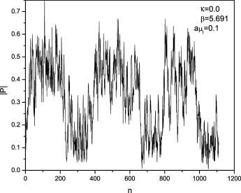
Figure 15: MC history of the Polyakov loop norm at $a\mu_{I}=0.1$, $\beta=5.691$, and $\kappa=0$.

Figure 16: MC history of the Polyakov loop norm at $a\mu_{I}=0.1$, $\beta=5.68$, and $\kappa=0.001$.

Figure 17: MC history of the Polyakov loop norm at $a\mu_{I}=0.1$, $\beta=4.736$, and $\kappa=0.17$.

Figure 18: Chiral condensate susceptibility as a function of $\beta$ at $a\mu_{I}=0.1$ and $\kappa=0.25$.

Figure 19: Susceptibility of the Polyakov loop norm as a function of $\beta$ at $a\mu_{I}=0.1$ and $\kappa=0.25$.

V PHASE DIAGRAM ON THE $(\mu,T)$ PLANE: THE PHYSICAL CASE

Replacing $\mu_{I}$ by $-i\mu$, we directly continue the transition line (12) at $\kappa=0.15$ from imaginary chemical potential to real chemical potential:

$$\beta_{C}=5.169(9)-0.954(33)\left(a\mu\right)^{2}+O\left(a^{4}\mu^{4}\right).$$ (13)

In order to translate the lattice results into the physical units, we use the renormalization group relation between the lattice spacing $a$ and $\beta$. The two loop perturbative expression givesCucchieri:2000hv

$$a\Lambda_{L} = \exp\bigg{(}-\frac{4\pi^{2}}{33-2N_{f}}\beta$$ (14)

$$+ \frac{459-57N_{f}}{(33-2N_{f})^{2}}\ln\left(\frac{8\pi^{2}}{33-2N_{f}}\beta\right)\bigg{)},$$ (15)

where $\Lambda_{L}$ is the lattice QCD scale. In Ref. Karsch:2000kv , the phase transition was studied with different kinds of fermion actions at $\mu=0$ and consistent results were obtained. Therefore we fix the lattice QCD scale by the critical temperature $T_{C}=164$ MeV at $\mu=0$ with 4 flavors for KS fermions Cucchieri:2000hv . The temperature $T$ is related to $a$ and $N_{t}$ by $T=1/(aN_{t})$. The critical line on the $(\mu,T)$ plane is shown in Fig. 20. For comparison, the critical line for KS fermionsD'Elia:2002gd is also shown. Within error bars, the results are consistent.

Figure 20: Phase diagram on the $(\mu,T)$ plane for $\kappa=0.15$. The area between the two solid lines is our result for Wilson quarks with error band, derived from Eqs. (13) and (14). The area between the two dotted lines is the result for KS fermions by D’Elia and Lombardo.

VI DISCUSSIONS

In the preceding sections, we have studied the properties of the phase structure of four-flavor QCD on the $(\mu,T)$ plane, using the information obtained from MC simulations of LGT with Wilson fermions at imaginary chemical potential $i\mu_{I}<i\pi T/3$.

The advantages of Wilson formulation have been mentioned in the introduction: it is free of species doubling and there is one to one correspondence between the flavors on the lattice and in the continuum.

Our study suggests that QCD with four flavors of Wilson quarks experiences a first order phase transition from the confinement phase to the deconfinement phase at small or large quark mass. However, at intermediate quark mass, the transition becomes a crossover. The properties of the transition are similar to those of KS fermions. This region is of interest for the present heavy-ion collision experiments.

Figure 21 is the expected phase diagram of lattice QCD with Wilson fermions in the $(\mu,T,\kappa)$ parameter space. There is a surface $\kappa=\kappa_{chiral}$ where the pion becomes massless. Above this surface, there is no phase transition, as confirmed by our numerical simulations for $\kappa=0.25$. Interesting physics is below this surface: at each $\kappa$, one should see a phase structure similar to Fig. 20. Of course, the order of transition depends on the value of $\kappa$. Due to heavy computational costs of simulations with dynamical fermions, we did not do a comprehensive search for the exact location of $\kappa_{1}$, $\kappa_{2}$ and $\kappa_{chiral}$. We believe that $\kappa_{1}\in(0.001,0.15)$, $\kappa_{2}\in(0.15,0.165)$ and $\kappa_{chiral}\in(0.17,0.25)$.

For lower temperature and larger chemical potential, all available MC simulation techniques fail. In the Hamiltonian lattice formulation, there has been successful analysis of the critical behavior for strong coupling QCD Gregory:1999pm ; Luo:2000xi ; Fang:2002rk at $(\mu,T=0)$ and on the $(\mu,T)$ planeLuo:2004mc . To study the continuum physics, new methods have to be developed. We hope to study these issues, as well as the dependence of the phase structure on the quark flavors, in the near future.

Figure 21: Expected phase diagram of lattice QCD with four flavors of Wilson quarks in the $(\mu,T,\kappa)$ parameter space. For $\kappa\in[0,\kappa_{1}]$ and $\kappa\in[\kappa_{2},\kappa_{chiral}]$, the phase transition is of first order, and while for $\kappa\in(\kappa_{1},\kappa_{2})$, the transition is a crossover.

- (1) S. Muroya, A. Nakamura, C. Nonaka and T. Takaishi, Prog. Theor. Phys. 110, 615 (2003), and refs. therein.
- (2) S. D. Katz, Nucl. Phys. B (Proc. Suppl.) 129, 60 (2004), and refs. therein.
- (3) M. P. Lombardo, Prog. Theor. Phys. Suppl. 153, 26 (2004), and refs. therein.
- (4) Z. Fodor and S. D. Katz, JHEP 0203, 014 (2002).
- (5) H. Neuberger, Phys. Rev. D 70, 097504 (2004).
- (6) B. Bunk, M. Della Morte, K. Jansen and F. Knechtli, Nucl. Phys. B 697, 343 (2004).
- (7) K. G. Wilson, Phys. Rev. D 10 (1974) 2445.
- (8) X. Q. Luo, Phys. Rev. D 70, 091504 (2004) (Rapid Commun.).
- (9) H. Neuberger, Phys. Lett. B 417, 141 (1998)
- (10) Z. Fodor, S. D. Katz and K. K. Szabo, JHEP 0408, 003 (2004)
- (11) P. Hasenfratz and F. Karsch, Phys. Lett. B 125, 308 (1983).
- (12) Z. Fodor and S. D. Katz, Phys. Lett. B 534, 87 (2002).
- (13) M. P. Lombardo, Nucl. Phys. B (Proc. Suppl.) 83, 375 (2000).
- (14) V. Azcoiti, G. Di Carlo, A. Galante and V. Laliena, JHEP 0412, 010 (2004).
- (15) A. Roberge and N. Weiss, Nucl. Phys. B 275, 734 (1986).
- (16) P. de Forcrand and O. Philipsen, Nucl. Phys. B 642, 290 (2002).
- (17) M. D’Elia and M. P. Lombardo, Phys. Rev. D 67, 014505 (2003).
- (18) S. A. Gottlieb, W. Liu, D. Toussaint, R. L. Renken and R. L. Sugar, Phys. Rev. D 35, 2531 (1987).
- (19) X. Q. Luo, E. B. Gregory, J. C. Yang, Y. L. Wang, D. Chang and Y. Lin, arXiv:hep-lat/0011090.
- (20) X. Q. Luo, E. B. Gregory, H. J. Xi, J. C. Yang, Y. L. Wang, Y. Lin and H. P. Ying, Nucl. Phys. B(Proc. Suppl.) 106, 1046 (2002).
- (21) A. Cucchieri and D. Zwanziger, Phys. Rev. D 65, 014002 (2002).
- (22) F. Karsch, E. Laermann and A. Peikert, Nucl. Phys. B 605, 579 (2001).
- (23) E. B. Gregory, S. H. Guo, H. Kröger and X. Q. Luo, Phys. Rev. D 62, 054508 (2000).
- (24) X. Q. Luo, E. B. Gregory, S. H. Guo and H. Kröger, hep-ph/0011120.
- (25) Y. Fang and X. Q. Luo, Phys. Rev. D 69, 114501 (2004).
- (26) http://physics.utah.edu/detar/milc/