Abstract

We present a scaling analysis in the 1-flavor Schwinger model with the full overlap and the rooted staggered determinant. In the latter case the chiral and continuum limit of the scalar condensate do not commute, while for overlap fermions they do. For the topological susceptibility a universal continuum limit is suggested, as is for the partition function and the Leutwyler-Smilga sum rule. In the heavy-quark force no difference is visible even at finite coupling. Finally, a direct comparison between the complete overlap and the rooted staggered determinant yields evidence that their ratio is constant up to $O(a^{2})$ effects.

1 Introduction

An issue which is of both phenomenological and conceptual relevance is whether it is a valid approach to use the staggered action to study QCD with ${N_{\!f}}\!=\!2$ or ${N_{\!f}}\!=\!2+1$ dynamical quarks. This is because the staggered Dirac operator $D^{\mathrm{st}}$ leads to 4 degenerate flavors in the continuum, and the simulations are thus performed by taking the square root of the staggered determinant (plus a quartic root for the dynamical strange quark). While the results of such studies look very promising from the phenomenological viewpoint [2, 3], a field-theoretic justification of the rooting procedure might be hard to find. The origin of the problem is that no one has constructed, so far, a local operator which, when raised to the fourth power, reproduces $D^{\mathrm{st}}$.

It has been shown that the most naive choice results in a non-local operator [4, 5], but of course a more elaborate construction might settle the issue.

The evidence in favor of the rooting procedure that comes from NLO staggered chiral perturbation theory [6] needs to be backed by numerical checks of the associated predictions (some are established [3]), and the analytical thoughts in [7] involve a number of simplifications. It has been shown – both in 2D and in 4D – that staggered eigenvalues on smooth enough backgrounds form near-degenerate pairs/quadruples which (apart from a rescaling factor) mimic the (non-degenerate) overlap eigenvalues on the same configuration [8, 9]. And the consequence that rooted staggered fermions satisfy an approximate index theorem and are in the right random-matrix universality class has been explicitly verified [10, 11]. However, all these pieces are inconclusive, as they do not say how the rooting procedure should be matched in the valence sector.

In the absence of a strict analytic argument, only a careful scaling study has some conceptual power, albeit an asymmetric one. If a continuum limit is found with rooted staggered fermions which agrees with another approach which is considered conceptually proof, nothing firm can be said (albeit a failure of the staggered framework seems less likely then). On the other hand, if the continuum limits disagree, the staggered answer would be in conflict with universality. In this note we attempt such a scaling study. The safe approach against which we shall compare is the overlap formulation [12], which, however, is far more demanding in terms of CPU time. The theory in which we will work is the massive ${N_{\!f}}\!=\!1$ Schwinger model, i.e. just QED in 2D.

We define the massless overlap operator as [12]

$$D^{\mathrm{ov}}=\rho\,\Big{(}1+\gamma_{5}\,\mathrm{sign}(\gamma_{5}D^{\mathrm{W}}_{-\rho})\Big{)}=\rho\,\Big{(}1+{D^{\mathrm{W}}_{-\rho}\over\sqrt{{D^{\mathrm{W}}_{-\rho}}^{\dagger}D^{\mathrm{W}}_{-\rho}}}\Big{)}$$ (1)

with $D^{\mathrm{W}}_{-\rho}$ the Wilson operator at negative mass $-\rho$, and construct the massive overlap via

$$D^{\mathrm{ov}}_{m}=(1\!-{m\over 2\rho})D^{\mathrm{ov}}+m\;.$$ (2)

The massless operator (1) satisfies the Ginsparg-Wilson relation [13]

$$D\hat{\gamma}_{5}+\gamma_{5}D=0,\qquad\hat{\gamma}_{5}=\gamma_{5}(1-{1\over\rho}D)$$ (3)

which substitutes the continuum chiral symmetry by the lattice chiral symmetry group [14]

$$\delta\psi=\hat{\gamma}_{5}\psi,\qquad\delta\overline{\psi}=\overline{\psi}\gamma_{5}$$ (4)

which, in turn, excludes additive mass renormalization and prevents operators in different chiral multiplets from mixing. On the lattices considered below, the full Dirac matrix may be kept in memory, and one can use standard linear algebra routines to perform a singular value decomposition of the shifted Wilson Dirac operator $D^{\mathrm{W}}_{-\rho}\!=\!USV^{\dagger}$, where $U,V$ are unitary matrices and $S\!>\!0$ is diagonal. The massless overlap operator is then simply given by

$$D^{\mathrm{ov}}\!=\!\rho(1+UV^{\dagger})$$ (5)

and it is straightforward to plug in a mass, see (2), and call further library routines to determine the complete eigenvalue spectrum. In practice, one may prefer to determine the eigensystem of ${D^{\mathrm{W}}_{-\rho}}^{\dagger}D^{\mathrm{W}}_{-\rho}$ or of $\gamma_{5}D^{\mathrm{W}}_{-\rho}$, but this does not bring any change in principle. We use $\rho\!=\!1$, which we checked, following Ref. [15], is an almost optimal choice with respect to locality for $\beta\!\geq\!4$.

The massless staggered operator reads

$$D^{\mathrm{st}}={1\over 2}\sum_{\mu}\eta_{\mu}(x)\Big{(}U_{\mu}(x)\delta_{x+\hat{\mu},y}-U_{\mu}^{\dagger}(x\!-\!\hat{\mu})\delta_{x-\hat{\mu},y}\Big{)}$$ (6)

with $\eta_{\mu}(x)\!=\!(-1)^{\sum_{\nu<\mu}x_{\nu}}$, and the massive operator is simply $D^{\mathrm{st}}_{m}\!=\!D^{\mathrm{st}}\!+\!m$. What remains of the continuum $SU(4)_{A}$ chiral symmetry group in the case of (6) is the abelian

$$\chi(x)\to\exp\Big{(}\mathrm{i}\,\theta_{A}(-1)^{\sum_{\nu}x_{\nu}}\Big{)}\chi(x)\quad,\qquad\bar{\chi}(x)\to\bar{\chi}(x)\exp\Big{(}-\mathrm{i}\,\theta_{A}(-1)^{\sum_{\nu}x_{\nu}}\Big{)}\;,$$ (7)

which, however, still protects the fermions against additive mass renormalization. The parallel transporter $U_{\mu}(x)$ in (6) may be replaced by a weighted sum of gauge-covariant paths from $x$ to $x\!+\!\hat{\mu}$ [16]. As a result, the most unphysical effects in the staggered formulation, the “taste-changing” interactions due to highly virtual gluon exchanges [17], can be considerably reduced. The reason is a separation of the relevant low-energy modes from the regularization dependent (and wildly fluctuating) high-energy modes and this is why we will speak of “UV-improved” or “UV-filtered” staggered quarks. For comparison the same modification will be considered in the overlap case [18, 8, 9], too, but there the effect will be much smaller.

We will be interested in the Schwinger model (SM) with one active flavor, since only there the rooting issue exists (in 2D the staggered formulation generates 2 flavors in the continuum), but for completeness let us mention the relationship to QCD both for ${N_{\!f}}\!=\!1$ and ${N_{\!f}}\!\geq\!2$.

In the zero temperature SM with ${N_{\!f}}\!=\!1$ the scalar condensate $\chi_{\mathrm{sca}}\!=\!\langle\overline{\psi}\psi\rangle$ at zero quark mass follows from the global axial anomaly and is given by [19]

$${\chi_{\mathrm{sca}}(m\!=\!0)\over e}={\exp(\gamma)\over 2\pi^{3/2}}=0.1599\ldots$$ (8)

where $\gamma\!=\!0.5772...$ is the Euler constant. Finite temperature effects will reduce $\chi_{\mathrm{sca}}$ [20], but no temperature will be large enough to really make it vanish. In other words, for ${N_{\!f}}\!=\!1$ there is no chiral phase transition, and thus the situation in the SM is analogous to QCD with ${N_{\!f}}\!=\!1$.

With ${N_{\!f}}\!\geq\!2$ and a small mass term the zero temperature SM shows a vague similarity to QCD slightly above the phase transition: The Polyakov loop does not vanish, and the chiral condensate is almost zero; the system “tries” to break the axial flavor symmetry spontaneously, the spectrum shows a gap between the “Schwinger particle” with mass $e\sqrt{{N_{\!f}}/\pi}\!+\!O(m)$ (the analog of the $\eta^{\prime}$) and the ${N_{\!f}}^{2}\!-\!1$ light “Quasi-Goldstones” with mass $M_{\pi}\!\sim\!m^{{N_{\!f}}/({N_{\!f}}+1)}$ [21]. The latter get sterile in the chiral limit (as required by Coleman’s theorem [22]), but the important point is that, as long as one stays away from the chiral limit, these “pions” dominate the correlators between external $P$- and $A_{\mu}$-sources at sufficiently long distance.

A peculiarity of any 2D gauge theory is that the fundamental coupling has the dimension of a mass. Furthermore, the SM is super-renormalizable and the coupling $e$ does not run, hence the theory is not asymptotically free. We use these features in taking the liberty to set the scale through $e$. In the compact lattice formulation, the fundamental charge is related to $\beta$ via

$$\beta={1\over(ae)^{2}}\;,$$ (9)

(below we will set $a\!=\!1$) and this means that the physical scale in the full theory depends only on $\beta$ and not on the fermion mass $m$. Of course, other choices would have been possible. One might set the scale via the measured slope in the short-distance potential (which is finite in 2D, since $\lim_{r\to 0}V(r)/r\!=\!\mathrm{const}$ in the continuum with a constant independent of ${N_{\!f}}$). In fact, our choice is just this short-distance option, up to cut-off effects.

2 Eigenvalue spectra

geometry	$8\!\times\!8$	$12\!\times\!12$	$16\!\times\!16$	$20\!\times\!20$	$24\!\times\!24$	$28\!\times\!28$
$\beta$	$0.8$	$1.8$	$3.2$	$5.0$	$7.2$	$9.8$
statistics	10,000	10,000	10,000	10,000	10,000	10,000

Table 1: Survey of matched zero temperature lattices, with statistics for both types of fermions.

geom.	$8\!\times\!2$	$16\!\times\!4$	$24\!\times\!6$	$32\!\times\!8$	$40\!\times\!10$	$48\!\times\!12$	$56\!\times\!14$	$64\!\times\!16$	$72\!\times\!18$	$80\!\times\!20$
$\beta$	$0.8$	$3.2$	$7.2$	$12.8$	$20.0$	$28.8$	$39.2$	$51.2$	$64.8$	$80.0$
over.	$\!10,\!000\!$	$\!10,\!000\!$	$\!10,\!000\!$	$\!10,\!000\!$	$\!10,\!000\!$	–	–	–	–	–
stag.	$\!10,\!000\!$	$\!10,\!000\!$	$\!10,\!000\!$	$\!10,\!000\!$	$\!10,\!000\!$	$\!10,\!000\!$	$\!10,\!000\!$	$\!10,\!000\!$	$\!10,\!000\!$	$\!10,\!000$

Table 2: Survey of matched $T\!=\!L/4$ lattices, with statistics for overlap and staggered fermions.

The plan is to produce a quenched ensemble, to compute all eigenvalues of the massless $D^{\mathrm{ov}},D^{\mathrm{st}}$ on each configuration and to introduce the dynamical fermions through reweighting [23]. We prepared a variety of lattices with fixed physical volume, both at zero temperature (i.e. with a time-extent $T\!=\!L$ large compared to all correlation lengths) and at a temperature given via $T\!=\!L/4$, see Tables 2, 2 for details. In 2D standard APE-smearing already involves the full hypercube, and we give the staple and the original link weight 0.5 each. Technically, we thus apply a smearing step and evaluate the fermion matrix on the resulting background, but we consider it a modification of the fermion action. What is peculiar to the choice of setting the scale through $\sqrt{\beta}$ is that our lattices are still (exactly) matched after reweighting to ${N_{\!f}}\!=\!1,2$.

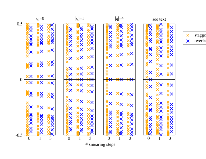
Figure 1: Low-energy spectrum of the unfiltered and two filtered versions of the Dirac operators $D^{\mathrm{st}}$ and $D^{\mathrm{ov}}$ [after chiral rotation as in (13)] on three typical configurations at $\beta\!=\!7.2$ and on a selected one where the overlap charge depends on the smearing level (rightmost panel).

Fig. 1 shows the low-energy spectrum of $D^{\mathrm{st}}$ and the $\hat{\lambda}$ of $D^{\mathrm{ov}}$ [cf. eqn. (13)] on four selected configurations at $\beta\!=\!7.2$. We define their topological charge as the overlap index [24, 14]

$$q(U)=\mathrm{ind}(U)={1\over 2\rho}\mathrm{tr}(\gamma_{5}D^{\mathrm{ov}})\;.$$ (10)

The first three are typical for topological charge $q=0,1,4$, respectively, while the last panel shows one of the rare (at $\beta\!=\!7.2$) cases where the overlap charge (10) depends on the filtering level or, likewise, on the parameter $\rho$. Without smearing there is a vague similarity between the staggered and the overlap spectrum on the $q\!=\!0$ configuration, but not on those with higher charge. This holds for fairly smooth gauge fields; the plaquette is $0.927722(54)$ at $\beta\!=\!7.2$. However, after a single smearing step, the situation improves dramatically. The staggered eigenvalues form near-degenerate pairs which sit close to an individual overlap eigenvalue. In particular the right number of “would-be” zero modes separates from the rest of the spectrum and clusters near the origin, namely $0,2,8$ for $q\!=\!0,1,4$, respectively. This is a manifestation of the (approximate) index theorem for staggered fermions which holds both in 2D [8] and in 4D [10, 9, 11]. However, the similarity extends to the higher modes, and one can take the “fingerprint” of a configuration likewise with $D^{\mathrm{ov}}$ or $D^{\mathrm{st}}$, the two differ just by a trivial rescaling factor and the two-fold degeneracy in the latter case. This is the basis of the rooting procedure for staggered fermions, and it is thus interesting to perform, in a first step, a scaling analysis for some observables which can be formed from the eigenvalues only.

3 Scalar condensate

For overlap fermions, the (bare) scalar condensate is unambiguously defined as [25]

$${\chi_{\mathrm{sca}}\over e}=-{\sqrt{\beta}\over L^{2}}\langle\overline{\psi}({1\over 2}+{\gamma_{5}\hat{\gamma}_{5}\over 2})\psi\rangle=-{\sqrt{\beta}\over L^{2}}\langle\overline{\psi}(1-{1\over 2\rho}D^{\mathrm{ov}})\psi\rangle\;.$$ (11)

Denoting the eigenvalues of the massless overlap Dirac operator by $\lambda$, and remembering that we work with $\rho\!=\!1$, the reweighted condensate is

$${\chi_{\mathrm{sca}}\over e}={\sqrt{\beta}\over L^{2}}{\langle\det(D^{\mathrm{ov}}_{m})^{N_{\!f}}\sum{1-\lambda/2\over(1-m/2)\lambda+m}\rangle\over\langle\det(D^{\mathrm{ov}}_{m})^{N_{\!f}}\rangle}\;,\qquad\det(D^{\mathrm{ov}}_{m})=\prod((1\!-\!{m\over 2})\lambda\!+\!m)$$ (12)

where the sum runs over the full spectrum. These eigenvalues occur either in complex conjugate pairs or as isolated chiral (doubler) modes at $\lambda\!=\!0\,(2)$. Finally, one can rewrite (12) as

$${\chi_{\mathrm{sca}}\over e}={\sqrt{\beta}\over L^{2}}{\langle\det(D^{\mathrm{ov}}_{m})^{N_{\!f}}\sum^{\prime}{1\over\hat{\lambda}+m}\rangle\over\langle\det(D^{\mathrm{ov}}_{m})^{N_{\!f}}\rangle}\;,\qquad\hat{\lambda}=\Big{(}\lambda^{-1}-2^{-1}\Big{)}^{-1}$$ (13)

where $\hat{\lambda}$ is purely imaginary and the primed sum excludes the doubler modes at $\lambda\!=\!2$.

In the staggered case we follow [26] and implement the (bare) 1-flavor condensate through

$${\chi_{\mathrm{sca}}\over e}=-{\sqrt{\beta}\over 2L^{2}}\langle\bar{\chi}\chi\rangle\;,$$ (14)

where the purpose of the factor $1/2$ is to compensate the two-fold degeneracy of the staggered formulation in 2D. Denoting the eigenvalues of the massless staggered Dirac operator by $\lambda$ (they show up in complex conjugate pairs with zero real part), the reweighted condensate is

$${\chi_{\mathrm{sca}}\over e}={\sqrt{\beta}\over 2L^{2}}{\langle\det(D^{\mathrm{st}}_{m})^{{N_{\!f}}/2}\sum{1\over(\lambda+m)}\rangle\over\langle\det(D^{\mathrm{st}}_{m})^{{N_{\!f}}/2}\rangle}\;,\qquad\det(D^{\mathrm{st}}_{m})=\prod(\lambda\!+\!m)\;.$$ (15)

with the sum and product running over the entire spectrum.

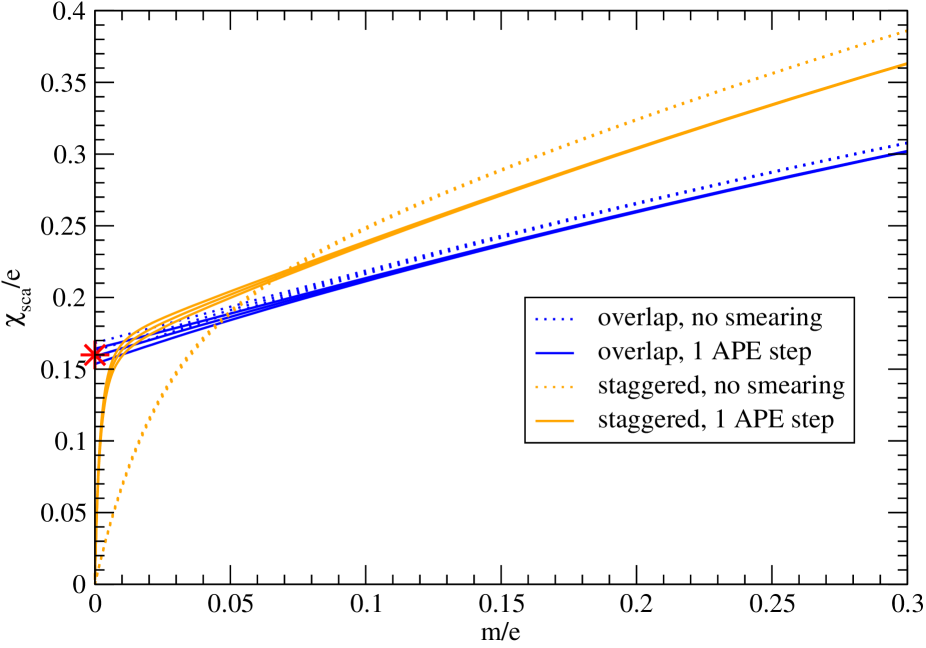
Figure 2: Bare overlap and rooted staggered ${N_{\!f}}\!=\!1$ condensate $\chi_{\mathrm{sca}}/e$ at $\beta\!=\!7.2$, plotted versus the quark mass. Here and in subsequent figures, three lines indicate a $1\sigma$-error band. The overlap result changes little, if a UV filtered Wilson operator is used instead of an unfiltered kernel. By contrast, in the staggered case this makes a big difference – only the filtered variety shows a clear separation into a regime (here: $m/e\!>\!0.02$) where the staggered answer is meaningful, and a regime ($m/e\!<\!0.02$) where lattice artefacts overwhelm.

Finally, there is no renormalization factor to be taken into account in a 2D theory with cut-off effects of order $O(a^{2})$, if one insists on a massless renormalization scheme. This follows from the general expansion $Z\!=\!1\!+\!O(e^{2})$ which, due to the dimensionful coupling, reads $Z\!=\!1\!+\!O(a^{2}e^{2})$ and thus tells us that there is no way to separate a $Z$-factor from intrinsic $O(a^{2})$ effects.

An example of the condensates (13, 15) with ${N_{\!f}}\!=\!1$ in one of our zero temperature geometries is shown in Fig. 2. The overlap yields a smooth curve which, for $m\!\to\!0$, is consistent with the Schwinger value (8), marked by an asterisk. This holds both with a standard Wilson kernel and with the filtered version. By contrast, the staggered condensate (at any filtering level and any $\beta$) tends to zero, if the chiral limit is performed at fixed lattice spacing, and taking, in a second step, the continuum limit will not change this, thus

$$\lim_{a\to 0}\lim_{m\to 0}{\chi_{\mathrm{sca}}^{\mathrm{st}}(m,a)\over e}=0\;.$$ (16)

Given the dramatic difference between the two staggered curves in Fig. 2, one wonders whether the staggered answer could be useful, if one uses only the data above some $m_{\mathrm{min}}$ to extrapolate to the chiral limit. Obviously, there is no canonical definition of such a $m_{\mathrm{min}}$, but the staggered results in Fig. 2 suggest that it might be less ambiguous for the filtered operator. The question can be formalized by asking whether it is possible to reproduce the Schwinger result (8) with rooted staggered fermions, if one considers the reverse order of limits, i.e. whether

$$\lim_{m\to 0}\lim_{a\to 0}{\chi_{\mathrm{sca}}^{\mathrm{st}}(m,a)\over e}={\exp(\gamma)\over 2\pi^{3/2}}\;.$$ (17)

The goal is to show that (only) the second order of limits works with staggered fermions, while the overlap discretization is correct with either order.

It turns out that eqn. (17) together with our definitions for $\chi_{\mathrm{sca}}^{\mathrm{ov/st}}$ does not make sense, neither for staggered nor for overlap fermions. This is because the definitions (11) and (14), when evaluated with a positive quark-mass, lead to a logarithmic divergence in the cut-off.

The logarithmic divergence shows up only in the condensate at finite $m$, with a coefficient that vanishes as the quark mass tends to zero. That such a “soft breaking” through $m\log(\Lambda^{2})$ terms must happen is obvious from the free case, where elementary manipulations yield

$$\langle\overline{\psi}\psi\rangle\! \!=\! \!\int\!d^{2}p\;{1\over p/-m}\,=\int\!d^{2}p\,{m\over p^{2}+m^{2}}\,=\int_{0}^{2\pi}\!d\varphi\int_{0}^{\infty}\!d\lambda\;{\lambda m\over\lambda^{2}+m^{2}}$$ (18)

$$\!=\! \!2\pi\lim_{\Lambda\to\infty}\int_{0}^{\Lambda}\!d\lambda\;{\lambda m\over\lambda^{2}+m^{2}}=\lim_{\Lambda\to\infty}\pi\,m\log\Big{(}{\Lambda^{2}+m^{2}\over m^{2}}\Big{)}\;.$$

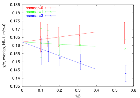
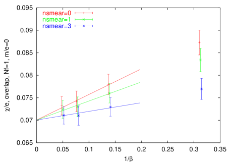
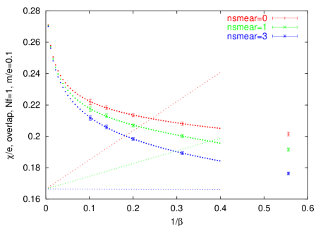
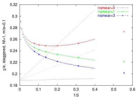
Figure 3: Bare overlap condensate $\chi_{\mathrm{sca}}^{\mathrm{ov}}/e$ with $m\!=\!0$ at zero temperature (left) or finite temperature (right) versus $(ae)^{2}$. The three filtering levels have a universal continuum limit, and the extrapolation (19) works well. The zero temperature result is consistent with (8).

Figure 4: Bare ${N_{\!f}}\!=\!1$ condensate $\chi_{\mathrm{sca}}/e$ with overlap (left) or rooted staggered (right) fermions at zero temperature and $m/e\!=\!0.1$ versus $(ae)^{2}$. The three filtering levels have a common logarithmic divergence. Adopting the ansatz (20), the divergence may be subtracted for either discretization, but the so-defined continuum limit is non-universal.

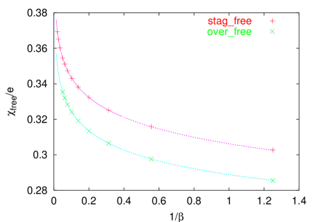
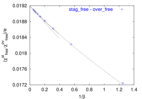
Figure 5: Left: Free condensates versus $1/\beta$ (in our zero temperature geometries, extended towards larger $\beta$), at fixed $m/e\!=\!0.1$. The fit to eqn. (21) uses the data below 0.4, i.e. $L\!\geq\!16$. Right: Difference of the free staggered and overlap condensate versus $1/\beta$. The data to the left of 0.4 are fitted with a $O(1/\beta)\!+\!O(1/\beta^{3/2})$ ansatz, shown together with its leading part.

Fig. 4 collects our ${N_{\!f}}\!=\!1$ overlap data at zero and finite temperature, evaluated at $m\!=\!0$. There is no sign of a logarithmic divergence, and we get an acceptable fit if we use

$${\chi_{\mathrm{sca}}(m\!=\!0,1/\beta,n)\over e}=A+B_{n}/\beta$$ (19)

with a common $A$ and slope parameters $B_{n}$ which account for the $O(a^{2})$ effects at filtering level $n$. At zero temperature our continuum result $A\!=\!0.1629(47)$ is compatible with the Schwinger value (8). The result $A\!=\!0.0700(16)$ from our thermal geometries indicates that at this temperature the massless continuum condensate is considerably reduced. The main lesson is that with overlap fermions one can indeed take the chiral limit first, letting $a\!\to\!0$ in a second step, and gets the correct answer.

Fig. 4 shows the ${N_{\!f}}\!=\!1$ zero temperature overlap and staggered condensates, evaluated at $m/e\!=\!0.1$. Now, the divergence in the cut-off is clearly visible. Indeed, we get an acceptable result from a correlated fit to all data (in one formulation) at fixed $m/e$ with the ansatz

$${\chi_{\mathrm{sca}}(m/e,1/\beta,n)\over e}=A+B_{n}/\beta+C\log(1/\beta)+(\delta_{n,0}D_{0}^{(3/2)}\!+\!\delta_{n,1}D_{1}^{(3/2)})/\beta^{3/2}+\delta_{n,0}D_{0}^{(2)}/\beta^{2}$$ (20)

where all coefficients depend on $m/e$, and $A,C$ are common to all filtering levels, while $B_{n}$, $D_{n}^{(3/2,2)}$ depend on the level $n$. Thus, besides the leading $O(a^{2})$ cut-off effects for each filtering level, we include $O(a^{3})$ terms in levels $1,0$, and $O(a^{4})$ terms with no smearing. With rooted staggered quarks everything is analogous, i.e. the ansatz (20) works again. The fine dotted lines beneath the data indicate what remains if one subtracts the so-determined logs plus higher order terms and stays with the constant plus linear part. For each $m/e\!>\!0$ there is a well-defined continuum limit with such a procedure, but there is no reason to expect it to be universal.

The difference between the “minimally subtracted” overlap and staggered condensates that survives in the continuum can be traced back to the difference between the two free condensates. The latter difference has a finite continuum limit, since each of the free condensates contains the same logarithmic divergence. This point is illustrated in Fig. 5. On the left the free condensates $\chi_{\mathrm{free}}^{\mathrm{ov/st}}/e$ at fixed physical quark mass are plotted versus $1/\beta$ (here, we refer to Tab. 2, i.e. $\beta$ merely encodes for the geometry). The curves have a common log term; they fit to the form

$${\chi_{\mathrm{free}}^{\mathrm{ov/st}}(m/e,1/\beta)\over e}=A_{\mathrm{free}}^{\mathrm{ov/st}}(m/e)+B_{\mathrm{free}}^{\mathrm{ov/st}}(m/e)/\beta+C_{\mathrm{free}}(m/e)\log(1/\beta)$$ (21)

where $A_{\mathrm{free}},B_{\mathrm{free}}$ depend on the discretization, while $C_{\mathrm{free}}$ is universal. The same conclusion is reached via directly plotting the difference, as shown on the right; the curvature decreases towards the continuum, and there is no sign of a remnant log.

The lesson is that one should define the massive continuum condensate in 2D through

$$\chi_{\mathrm{subt}}(m/e)=\int_{0}^{\infty}\!d\lambda\;{2m\over\lambda^{2}+m^{2}}\;\Big{[}\rho(\lambda)-\rho_{\mathrm{free}}(\lambda)\Big{]}$$ (22)

in infinite volume and regard its computation with overlap and staggered fermions a direct test of universality. Here, the underlying assumption is that asymptotically the eigenvalue density $\rho(\lambda)$ agrees with the free one [from a glimpse at (18), one learns that $\rho_{\mathrm{free}}(\lambda)\to\pi\lambda$].

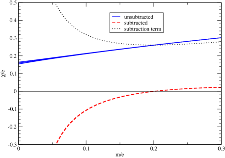
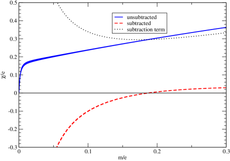
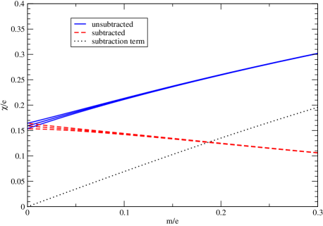
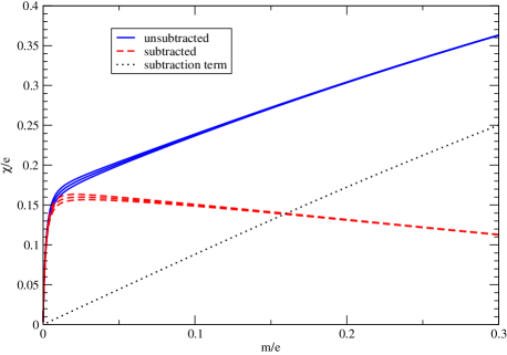
Figure 6: The “naive” subtracted condensates (25, 26) at $\beta\!=\!7.2$, together with $\chi_{\mathrm{sca}}$ and $\chi_{\mathrm{free}}$ for overlap (left) and staggered (right) fermions. Note the power-like IR-divergence in $\chi_{\mathrm{subt}}^{\mathrm{ov/st}}$.

Figure 7: The “primed” subtracted condensates (29, 30) at $\beta\!=\!7.2$. No IR-divergence is left.

A legitimate strategy to implement (22) on the lattice is to first subtract the free case in the same formulation and geometry, followed by an extrapolation to infinite volume. The first step may be done analytically, the corresponding expressions read

$$\chi_{\mathrm{free}}^{\mathrm{ov}}(m) = {1\over L^{2}}\sum_{k_{1},k_{2}=0}^{L-1}\mathrm{Tr}\!\left\{D_{\mathrm{free}}^{\mathrm{ov}}(m)^{-1}\Big{(}1-{1\over 2\rho}D_{\mathrm{free}}^{\mathrm{ov}}(0)\Big{)}\right\}$$ (23)

$$D_{\mathrm{free}}^{\mathrm{ov}}(m) = \Big{(}\rho-{m\over 2}\Big{)}\left(1+{D_{\mathrm{free}}^{\mathrm{W}}(-\rho)\over|D_{\mathrm{free}}^{\mathrm{W}}(-\rho)|}\right)+m$$

$$D_{\mathrm{free}}^{\mathrm{W}}(M) = 2+M-\sum_{\mu}c_{\mu}+\mathrm{i}\sum_{\mu}s_{\mu}\gamma_{\mu}$$

$$\chi_{\mathrm{free}}^{\mathrm{st}}(m) = {1\over L^{2}}\sum_{k_{1},k_{2}=0}^{L/2-1}{2m\over m^{2}+s_{1}^{2}+s_{2}^{2}}$$ (24)

with $c_{\mu}=\cos({2\pi\over L}k_{\mu})$ and $s_{\mu}=\sin({2\pi\over L}k_{\mu})$. In the (“naive”) subtracted condensates

$$\chi_{\mathrm{subt}}^{\mathrm{ov}}(m/e,1/\beta,V) = \chi_{\mathrm{sca}}^{\mathrm{ov}}(m/e,1/\beta,V)-\chi_{\mathrm{free}}^{\mathrm{ov}}(m/e,V)$$ (25)

$$\chi_{\mathrm{subt}}^{\mathrm{st}}(m/e,1/\beta,V) = \chi_{\mathrm{sca}}^{\mathrm{st}}(m/e,1/\beta,V)-\chi_{\mathrm{free}}^{\mathrm{st}}(m/e,V)$$ (26)

the limit $V\!\to\!\infty$ must be taken before $m\!\to\!0$, since the free case contains a massless mode, and this reflects itself in the behavior $\chi_{\mathrm{subt}}^{\mathrm{ov/st}}/e\!\to\!-2/(emV)$ for a small mass.

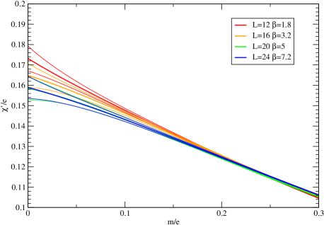
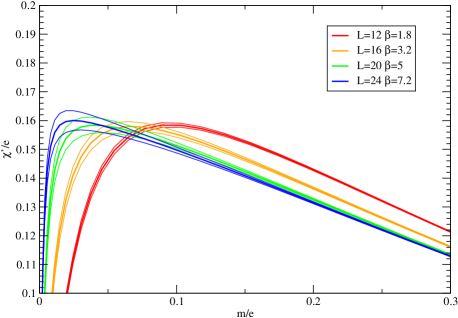
Figure 8: The “primed” subtracted condensates (29, 30) for overlap (left) and staggered (right) fermions with 1 smearing step. Note the small scaling violations at any $m/e$ with overlap fermions, while they get progressively worse for small $m/e$ in the staggered case.

Looking at (23, 24) the piece that makes the chiral limit in a finite volume singular is easily identified, it is the term with $k_{1}\!=\!k_{2}\!=\!0$. Hence, a better choice is to subtract the free case in the same geometry without the non-topological zero-modes. With

$$\chi_{\mathrm{free}}^{\prime\;\mathrm{ov}}(m) = {1\over L^{2}}\sum\nolimits^{\prime}\mathrm{Tr}\!\left\{D_{\mathrm{free}}^{\mathrm{ov}}(m)^{-1}\Big{(}1-{1\over 2\rho}D_{\mathrm{free}}^{\mathrm{ov}}(0)\Big{)}\right\}$$ (27)

$$\chi_{\mathrm{free}}^{\prime\;\mathrm{st}}(m) = {1\over L^{2}}\sum\nolimits^{\prime}{2m\over m^{2}+s_{1}^{2}+s_{2}^{2}}$$ (28)

[the primed sum skips the $(0,0)$ contribution, otherwise the summation is as in (23, 24)], one may define the “primed” subtracted condensates

$$\chi_{\mathrm{subt}}^{\prime\;\mathrm{ov}}(m/e,1/\beta,V) = \chi_{\mathrm{sca}}^{\mathrm{ov}}(m/e,1/\beta,V)-\chi_{\mathrm{free}}^{\prime\;\mathrm{ov}}(m/e,V)$$ (29)

$$\chi_{\mathrm{subt}}^{\prime\;\mathrm{st}}(m/e,1/\beta,V) = \chi_{\mathrm{sca}}^{\mathrm{st}}(m/e,1/\beta,V)-\chi_{\mathrm{free}}^{\prime\;\mathrm{st}}(m/e,V)$$ (30)

that avoid the IR singularity in (25, 26). In other words, (29, 30) is the only lattice implementation of (22) which is simultaneously UV and IR finite and thus permits to skip the limit $V\!\to\!\infty$, because finite volume corrections are (asymptotically) exponentially small. Note that this procedure differs from a standard renormalization in QCD. Since the theory is super-renormalizable, there is no bare parameter to be adjusted and no counterterm to be added to the Lagrangian, the only option is a pure vacuum reordering.

The “naive” and “primed” condensates (25, 26) and (29, 30) are shown for one coupling in Fig. 7 and Fig. 7, both for overlap and staggered quarks. The former version clearly exhibits the IR divergence $\chi_{\mathrm{subt}}^{\mathrm{ov/st}}(m/e\!\to\!0)/e\!\to\!-2/(emV)$, due to the subtraction term in (25, 26). In the latter version, the leading finite-volume effects are tied to the lightest particle in the interacting theory, the Schwinger particle with mass $e/\sqrt{\pi}\!+\!O(m)$, and thus exponentially small.

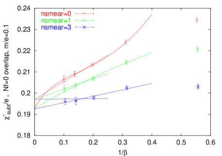
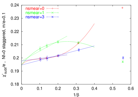
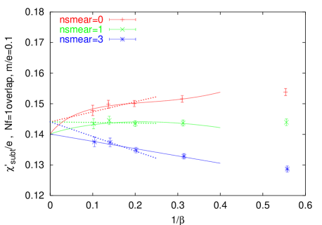
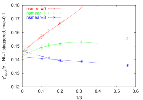
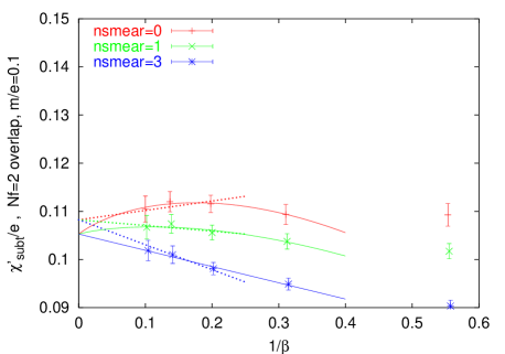
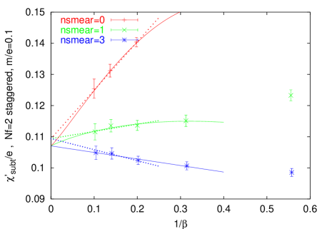
Figure 9: Continuum limit, via (20) without the log (full lines), of $\chi_{\mathrm{subt}}^{\prime}/e$ at fixed $m/e\!=\!0.1$ with overlap (left) and staggered (right) quarks for ${N_{\!f}}\!=\!0,1,2$ (top, center, bottom). Comparing to the strictly linear extrapolation (dotted lines) gives a measure for the systematic error.

Having defined the “primed” subtracted condensates, we are in a position to let, for any fixed $m/e\!>\!0$, the lattice spacing tend to zero

$${\chi_{\mathrm{cont}}^{\prime\;\mathrm{ov}}(m/e)\over e} = \lim_{1/\beta\to 0}\sqrt{\beta}\chi_{\mathrm{subt}}^{\prime\;\mathrm{ov}}(m/e,1/\beta)$$ (31)

$${\chi_{\mathrm{cont}}^{\prime\;\mathrm{st}}(m/e)\over e} = \lim_{1/\beta\to 0}\sqrt{\beta}\chi_{\mathrm{subt}}^{\prime\;\mathrm{st}}(m/e,1/\beta)$$ (32)

and Fig. 8 indicates that there is, at this stage, a practical difference among the two formulations. In the overlap case cut-off effects are mild, and this means that the continuum limit can be taken, from the $\beta$-values available, over the full mass range shown. With rooted staggered quarks, scaling violations get progressively worse for small $m/e$.

Fig. 9 indicates that, once the fermion mass is large enough to be in the staggered scaling regime, both formulations agree in the continuum, and the agreement seems not to be tied to a particular ${N_{\!f}}$. Comparing our (${N_{\!f}}\!=\!1$) continuum result $\chi_{\mathrm{cont}}^{\prime\;\mathrm{ov}}(m/e\!=\!0.1)\!=\!0.142(4)$ to the values 0.1171 by Hosotani [27] and 0.1277 by Adam [28] we find a disagreement at the $6.2\sigma$ or $3.6\sigma$ level, respectively. This might indicate a finite-volume effect or a limited precision of the latter calculations. Since our boxlength is $\sim\!5$ times larger than the correlation length of the lightest particle in the massless ${N_{\!f}}\!=\!1$ theory, and in this regime finite-volume effects are exponentially small [20], we consider the first option with our data unlikely.

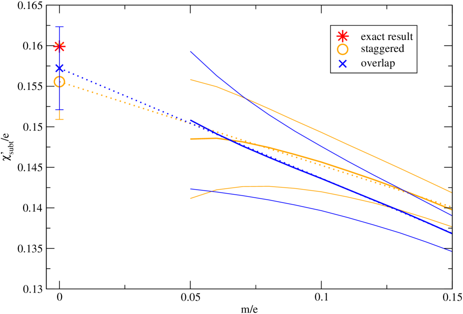
Figure 10: Chiral extrapolation of the continuum extrapolated primed condensates (31, 32). In the staggered case the continuum limit can only be taken for $m/e\!\geq\!0.05$ from our $\beta$-values, and with overlap quarks the same cut is applied for consistency. A linear extrapolation $m\!\to\!0$ agrees with the analytical result (8) for either discretization. The error-band is only statistical.

As a last step, one my now take the chiral limit. In the staggered case we find that after the $a\!\to\!0$ limit has been taken with the ansatz

$${\chi_{\mathrm{subt}}^{\prime}(m/e,1/\beta,n)\over e}=A+B_{n}/\beta+C\log(1/\beta)+D_{n}/\beta^{3/2}\;.$$ (33)

we have a continuum curve that covers the range $0.05\!\leq\!m/e\!\leq\!0.15$, outside the ansatz (33) yields an unacceptable $\chi^{2}$. Using this segment and a linear ansatz for the extrapolation ${m\!\to\!0}$ we find that the massless staggered ${N_{\!f}}\!=\!1$ condensate agrees with the analytical result (8). In the overlap case the continuum curve would extend to $m/e\!=\!0$, but as a consistency check we perform the same extrapolation, getting again a result compatible with (8). Both extrapolations are shown in Fig. 10. Thus, for overlap fermions our data support the universal behavior

$$\lim_{a\to 0}\lim_{m\to 0}{\chi_{\mathrm{subt}}^{\prime\;\mathrm{ov}}(m/e,a^{2})\over e}=\lim_{m\to 0}\lim_{a\to 0}{\chi_{\mathrm{subt}}^{\prime\;\mathrm{ov}}(m/e,a^{2})\over e}={\exp(\gamma)\over 2\pi^{3/2}}\;.$$ (34)

For staggered fermions, one the other hand, the suggested non-commutativity phenomenon

$$\lim_{a\to 0}\lim_{m\to 0}{\chi_{\mathrm{subt}}^{\prime\;\mathrm{st}}(m/e,a^{2})\over e}=0\quad,\qquad\lim_{m\to 0}\lim_{a\to 0}{\chi_{\mathrm{subt}}^{\prime\;\mathrm{st}}(m/e,a^{2})\over e}={\exp(\gamma)\over 2\pi^{3/2}}$$ (35)

means that rooted staggered fermions can be used to reproduce the Schwinger result (8), but only if the right order of limits is chosen.

4 Topological susceptibility

Another interesting observable to study the effects of dynamical fermions is the topological susceptibility which, in the context of this note, shall be defined (in the continuum) through

$$\chi_{\mathrm{top}}=\lim_{V\to\infty}{\langle\det(D\!+\!m)^{N_{\!f}}\;q^{2}\rangle\over V\,\langle\det(D\!+\!m)^{N_{\!f}}\rangle}\;.$$ (36)

The main difference to the scalar condensate is that the topological susceptibility depends only on the sea-quarks, thus offering a potentially cleaner view at the effects of square-rooting the staggered determinant to get ${N_{\!f}}\!=\!1$.

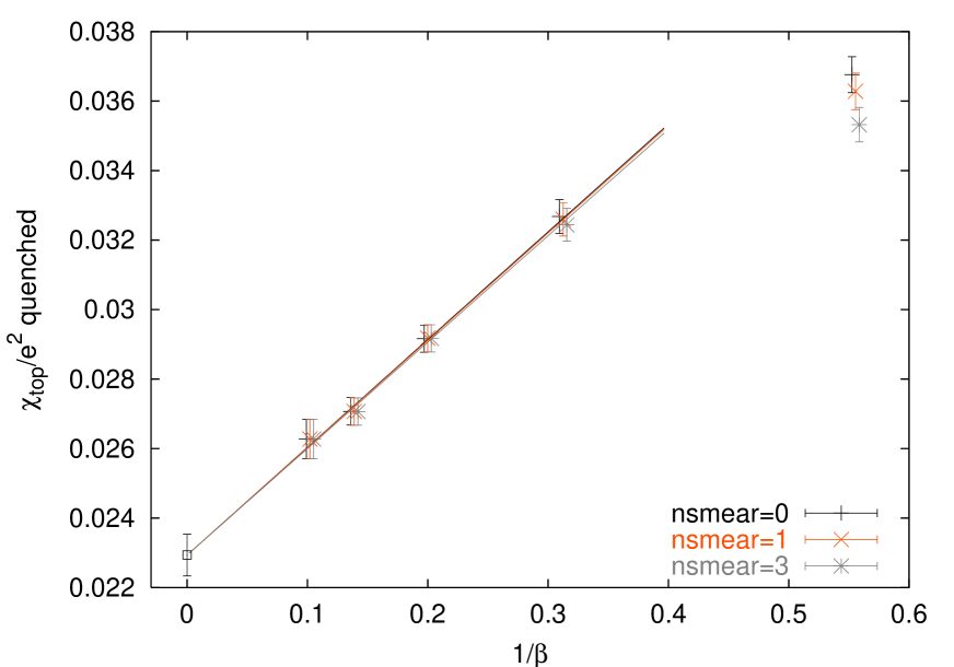
Figure 11: The zero temperature quenched topological susceptibility $\chi_{\mathrm{top}}^{{N_{\!f}}=0}/e^{2}$ versus $(ae)^{2}$. The symbols for $\mathrm{nsmear}\!=\!0,3$ are slightly offset for better visibility. Note the steep slope – in spite of being in the scaling regime for $\beta\!\geq\!3.2$, cut-off effects can be large. At $\beta\!=\!9.8$ the charge $q$ is independent of the smearing level for all our configurations.

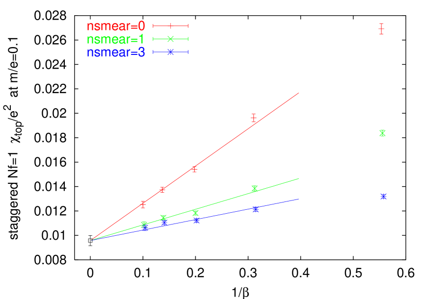
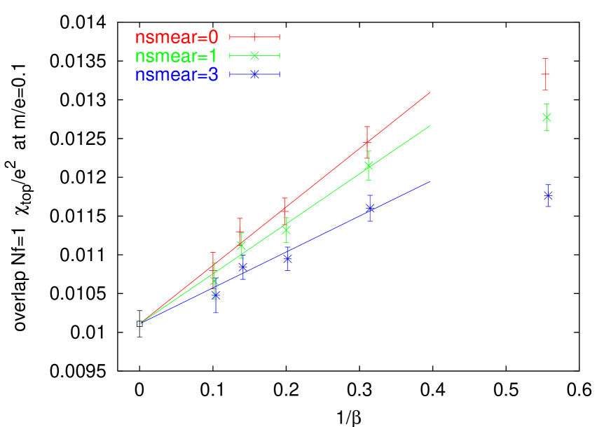
Figure 12: At the fixed quark mass $m/e\!=\!0.1$ a correlated fit to all staggered ${N_{\!f}}\!=\!1$ data (top) suggest a continuum limit 0.00958(42) which is consistent with 0.01011(17) from all overlap data (bottom). In the staggered case, the first smearing renders the extrapolation much flatter, while the overlap has a flat behavior with any level of filtering (note the difference in scale).

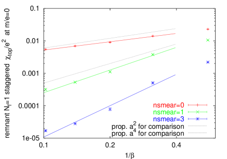
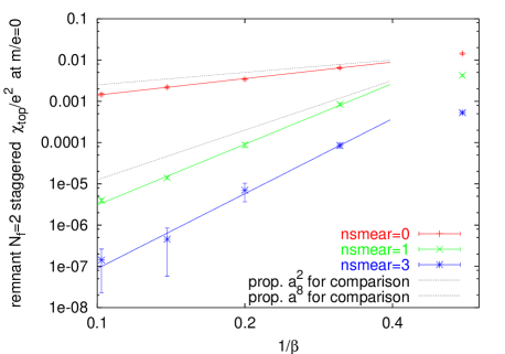
Figure 13: The remnant $\chi_{\mathrm{top}}^{\mathrm{st}}/e^{2}$ at $m/e\!=\!0$ versus $1/\beta$, in log-log scale. This staggered artefact seems to disappear with a power-law in $a$, for ${N_{\!f}}\!=\!1$ (left) and ${N_{\!f}}\!=\!2$ (right), but the power is 2 only for smearing level 0, while it is $4...8$ for higher filtering levels (over our range of $\beta$-values).

For staggered quarks, the definition (36), taken in fixed volume, reduces to

$${\chi_{\mathrm{top}}^{\mathrm{st}}\over e^{2}}={\beta\over L^{2}}\,{\langle\det(D^{\mathrm{st}}_{m})^{{N_{\!f}}/2}\;q^{2}\rangle\over\langle\det(D^{\mathrm{st}}_{m})^{{N_{\!f}}/2}\rangle}\;,$$ (37)

while for overlap quarks, the implementation is

$${\chi_{\mathrm{top}}^{\mathrm{ov}}\over e^{2}}={\beta\over L^{2}}\,{\langle\det(D^{\mathrm{ov}}_{m})^{N_{\!f}}\;q^{2}\rangle\over\langle\det(D^{\mathrm{ov}}_{m})^{N_{\!f}}\rangle}\;,$$ (38)

where $\det(D^{\mathrm{st}}_{m})$ and $\det(D^{\mathrm{ov}}_{m})$ are defined in (15, 12). The sum is over the full spectrum of the massless operator, and we apply the overlap definition (10) of the charge $q$ in either case.

Let us begin with a check that a reasonable number of our zero temperature $\beta$-values is in the scaling regime before reweighting. Fig. 11 contains our quenched topological susceptibility data, and $\beta\!\geq\!3.2$ seems sufficient to be in the regime with only $O(a^{2})$ effects.

The first test is whether overlap and rooted staggered quarks yield the same result in the continuum, if the topological susceptibility $\chi_{\mathrm{top}}^{{N_{\!f}}=1}(m/e)/e^{2}$ is taken at a fixed non-vanishing quark mass. Fig. 12 presents the outcome for $m/e\!=\!0.1$. In either case the three smearing levels seem to have a common continuum limit and this is why we adopt a correlated linear fit. The staggered continuum value 0.00958(42) is consistent with 0.01011(18) from all overlap data. This is of course not a proof but good numerical evidence that rooted staggered quarks yield the correct continuum limit for the topological susceptibility at finite quark mass.

The second test concerns the chiral limit, where $\chi_{\mathrm{top}}^{\mathrm{ov}}(0)\!=\!0$ (as in the continuum [29]), while $\chi_{\mathrm{top}}^{\mathrm{st}}(0)\!>\!0$ is a pure discretization effect. Fig. 13 shows the remnant staggered susceptibility at $m/e\!=\!0$ versus $(ae)^{2}$, in a log-log representation. With unfiltered staggered sea-quarks it seems to disappear in proportion to $a^{2}$, regardless of ${N_{\!f}}$. For the filtered variety we find a slope $\sim\!2$ (i.e. dominating $O(a^{4})$ cut-off effects) over the range of accessible couplings for ${N_{\!f}}\!=\!1$ and even $\sim\!4$ (i.e. dominating $O(a^{8})$ effects) for ${N_{\!f}}\!=\!2$. Still, it is conceivable that this slope eventually flattens out and the asymptotic cut-off effects might be $O(a^{2})$ with any level of filtering. This would mean that smearing renders the coefficient in front of the $O(a^{2})$ term so small that the “subleading” $O(a^{4})$ or $O(a^{8})$ terms would numerically dominate over a substantial range of couplings. In any case, the important news is that the non-commutativity phenomenon in the chiral condensate is not replicated here – for the topological susceptibility the staggered answer is correct even if the chiral limit is taken before the continuum limit.

5 Partition function and Leutwyler-Smilga sum rules

In the $\epsilon$-regime of QCD [29] ($m\Sigma V\!\ll\!1$, but still with a large box-size, i.e. $L\!\gg\!1/(2F_{\pi})\!\simeq\!1\,\mathrm{fm}$, c.f. the discussion in [30]) the log of the partition function is known analytically [29]

$$Z_{\theta}(m)=e^{m\Sigma V\cos(\theta)}$$ (39)

with sub-leading corrections of order $(m\Sigma V)^{2}$. The partition function in a sector of fixed topological charge $q$ follows by taking the Fourier transform [29]

$$Z_{q}(m)=\int d\theta\;e^{\mathrm{i}q\theta}Z_{\theta}(m)=I_{|q|}(m\Sigma V)$$ (40)

where $I_{|q|}$ is the modified Bessel function.

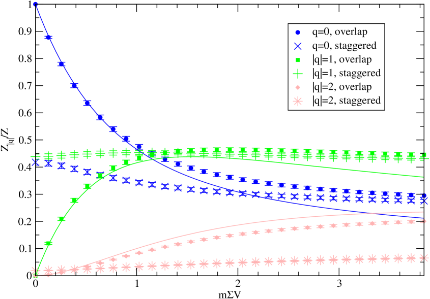
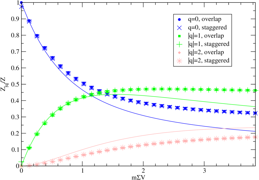
Figure 14: The ${N_{\!f}}\!=\!1$ partition function $Z_{|q|}$ (normalized by the sum over all $q$) at $\beta\!=\!3.2$ without filtering (top) and at $\beta\!=\!9.8$ with 1 smearing step (bottom) versus $x\!=\!m\Sigma V$. For sufficiently small mass the overlap version (filled symbols) is always a decreasing function of $|q|$, as in the continuum. The rooted staggered version (crosses) joins, for large mass, the associated overlap $Z_{|q|}/Z_{\theta=0}$. The full lines represent the parameter-free prediction (39, 40).

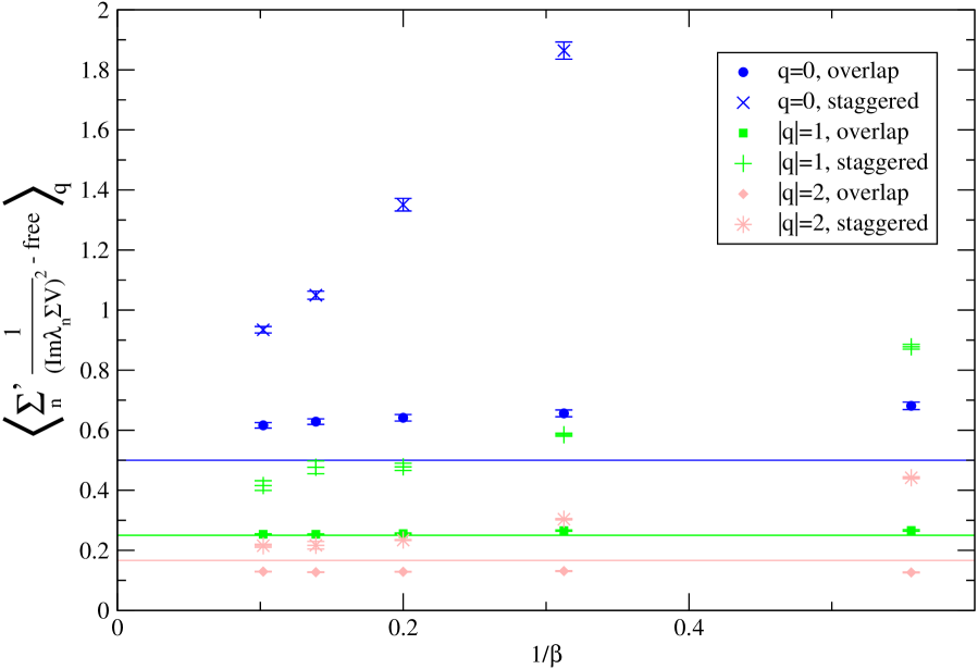
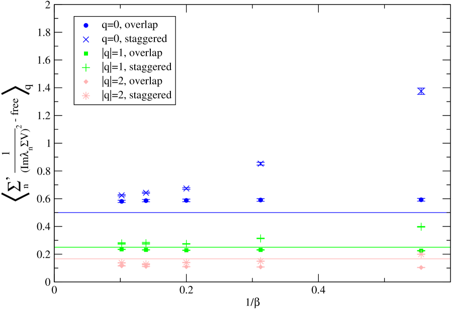
Figure 15: The Leutwyler-Smilga sum rule (42) for ${N_{\!f}}\!=\!1$ active quarks versus $(ae)^{2}$, at smearing level 0 (top) and 1 (bottom). Note the dramatic difference in the scaling behavior between overlap and rooted staggered fermions. The deviation, in the continuum, from the Leutwyler-Smilga prediction (full lines) is likely a finite-volume effect.

By differentiating with respect to the quark mass and setting the latter to zero, Leutwyler and Smilga obtained the first sum rule for the inverse eigenvalues of the massless Dirac operator

$$\left\langle\sum_{n}\nolimits^{\prime}{1\over(\mathrm{imag}(\lambda_{n})\Sigma V)^{2}}\right\rangle_{\!\!q}^{\!\!\prime}={1\over 2(|q|\!+\!{N_{\!f}})}$$ (41)

where the primes indicate that in a sector with topological charge $q\!\neq\!0$ the sum is over the full spectrum without the $|q|$ zero modes and the importance sampling is to be carried out with the “primed determinant”, i.e. without the zero modes. In 4D the l.h.s. is quadratically divergent, since the eigenmode distribution is asymptotically proportional to $\lambda^{3}$. In 2D the divergence is logarithmic, since the eigenmode distribution is asymptotically linear in $\lambda$ [cf. (22)]. One way out is to subtract the free case in the same volume. An other one is to consider the difference between two topological sectors, since the UV-behavior is independent of the charge.

We start with the conjecture that eqn. (39) and thus (40, 41) hold in the 1-flavor Schwinger model, too, albeit with re-interpreting $\Sigma$ as the analytically known 1-flavor condensate (8).

In Fig. 14 we show the ${N_{\!f}}\!=\!1$ partition function on a coarse and a fine lattice, without and with one APE step, respectively. In the first case, one sees a significant difference between the overlap and the rooted staggered answer for small quark masses. For larger $\beta$ and with just one smearing step this difference disappears and we did not find any indication for a disagreement in the continuum limit at any $m/e$. For $x\!\ll\!1$ the continuum extrapolated data agree well with $(2\!-\!\delta_{q,0})I_{|q|}(x)/\exp(x)$ which, with our choice for $\Sigma$, is a parameter-free prediction. We like to point out that this figure is reminiscent of the situation in QCD, see Fig. 3 of Ref. [31].

To verify (41) we subtract the free case, i.e. we check whether

$$\left\langle\sum_{n}\nolimits^{\prime}{1\over(\mathrm{imag}(\lambda_{n})\,\Sigma V)^{2}}-\sum_{n}\nolimits^{\prime}{1\over(\mathrm{imag}(\lambda_{n}^{\mathrm{free}})\,\Sigma V)^{2}}\right\rangle_{\!\!q}^{\!\!\prime}={1\over 2(|q|\!+\!{N_{\!f}})}$$ (42)

with $\lambda_{n}$ denoting the (purely imaginary) $n$-th staggered or chirally rotated overlap eigenvalue (i.e. the $\hat{\lambda}$ of (13)), and in the staggered case an additional factor $1/2$ on the l.h.s. is needed (or $1/4$ in 4D). The prime on the sum indicates that on topologically nontrivial configurations the $|q|$ true overlap zero modes or the $|q|$ “would be” zero modes on either side of the staggered spectrum are excluded. Since also the free overlap and staggered Dirac operators have 2 and 4 (non-topological) zero modes, respectively, the $\lambda_{n}^{\mathrm{free}}$ denote the free eigenvalues without these zeros. Thus the sum over $n$ does not include the same number of terms in the free and interacting case. The prime above the expectation value indicates that in a $q\!\neq\!0$ sector the $|q|$ zeros are removed from the determinant. Fig. 15 contains our results for the sum rule (42), where our choice for the interpretation of $\Sigma$ leads again to a parameter-free prediction. The deviation from the Leutwyler-Smilga value is likely a finite-volume effect. In any case, there is no sign of a difference between the rooted staggered and the overlap answer in the continuum.

6 Heavy quark potential

The heavy-quark (HQ) potential is an interesting observable, since it is easy to measure in the Schwinger model and the effect of dynamical fermions is clearly visible. We define the HQ potential $V(r)$ in a finite volume $L\times T$ via the Polyakov loop correlator

$$e^{-V(r)T}=\langle P(0)P^{\dagger}(r)\rangle\;.$$ (43)

In the quenched case, and with $T\!\to\!\infty$, it has a simple saw tooth shape, i.e. it starts at zero, raises linearly for $0\!\leq\!r\!\leq\!L/2$, and then it decreases linearly, until it reaches $0$ at $r\!=\!L$ again. This follows from the fact that the quenched Wilson loop in infinite volume satisfies an exact area law $W_{{N_{\!f}}=0}(r,t)=(I_{1}(\beta)/I_{0}(\beta))^{rt}$ [in lattice units], thus the force in physical units is

$${F_{{N_{\!f}}=0,T=\infty}(r)\over e^{2}}=-\beta\log\Big{(}{I_{1}(\beta)\over I_{0}(\beta)}\Big{)}\;.$$ (44)

In the ${N_{\!f}}\!=\!1$ case an exact solution on the torus is known for $m\!=\!0$ [20], but – as far as we know – not for massive fermions. However, we expect the screening behavior found in the massless case to also apply, on a qualitative level, for a small enough fermion mass.

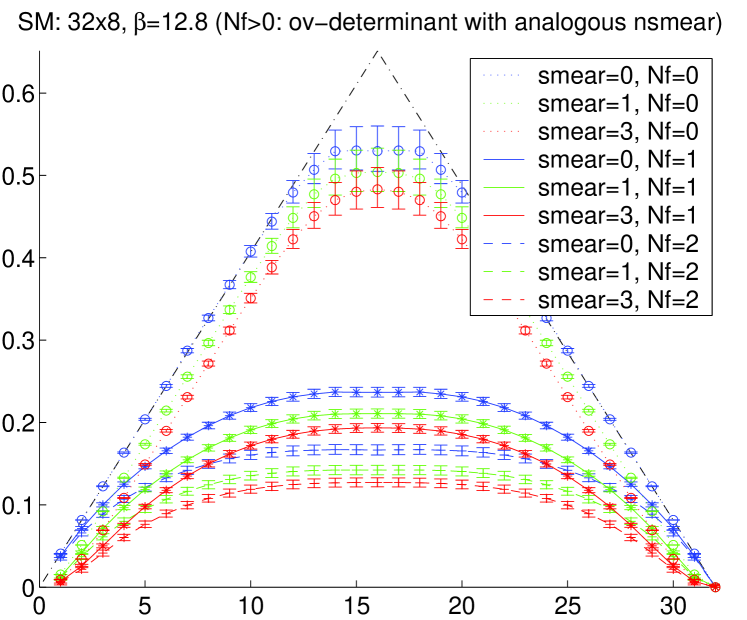
Figure 16: The quenched zero temperature HQ-potential is a saw tooth. After reweighting with staggered (top, rooted for ${N_{\!f}}\!=\!1$) or overlap (bottom) fermions ($m/e\!=\!0.1$), screening is seen. Throughout, the same smearing is applied in the HQ line and in the fermion operator. Except near the endpoints, the improved HQ action leads to a mere downwards shift of the potential.

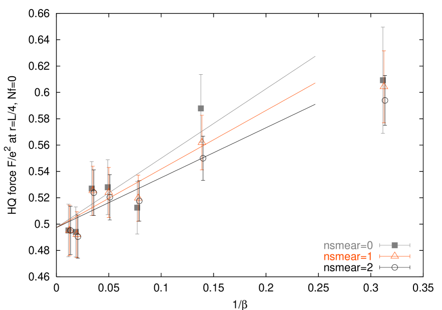
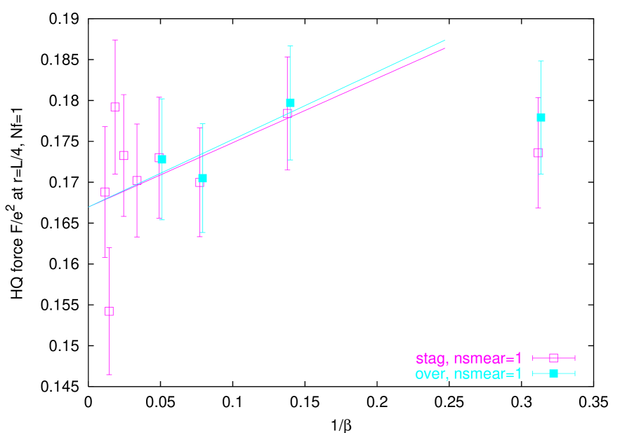
Figure 17: Top: With our $\beta$-values, the quenched heavy-quark force $F/e^{2}$ at $r\!=\!L/4$ is in the scaling regime. For large enough $\beta$, the three HQ actions agree in their central values and errors. Bottom: The ${N_{\!f}}\!=\!1$ HQ force $F/e^{2}$ at $r\!=\!L/4$ with overlap or rooted staggered fermions (filtering level 1 applied in both and the HQ action) seems to have a universal continuum limit.

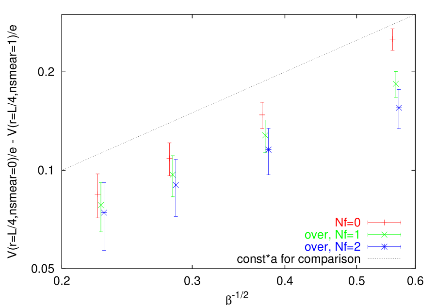
Figure 18: The difference between the HQ potentials with smearing-level 0 and 1 (at $r\!=\!L/4$) versus $ae$, in log-log scale. It disappears in proportion to $a$ – the offset line has slope 1.

In Fig. 16 we show an example of our HQ potentials ($\beta\!=\!12.8$, lattice units). In this regime the quenched prediction (44) works very well, except that the finite temperature causes a flattening of the peak region. If the Polyakov loops are built from smeared links instead of the original ones (“improved HQ action”, see [32, 33]), the potential is merely shifted downwards, except near $r=0,L$ where some curvature is introduced. In other words, the force is unaffected by such a modification of the HQ action, provided it is measured at a distance larger than the number of smearing steps applied. Furthermore, the reduced HQ selfenergy is supposed to lead to a smaller error bar (originally [32], see  [33] for details), but here it seems unaffected – we will come back to this point. After reweighting to ${N_{\!f}}\!=\!1$ or ${N_{\!f}}\!=\!2$, screening is seen (as expected), yet there is no visible difference between staggered (top) or overlap (bottom) dynamical flavors. Here we show only the “diagonal” data, where the same smearing level is applied in the HQ action as in the fermion operators, but the “offdiagonal” data are similar.

For a detailed analysis we shall concentrate on the force at a given (large enough) distance, and we choose to present a scaling analysis for $F_{{N_{\!f}}=1}(r\!=\!L/4)/e^{2}$. Before doing so, it is worthwhile to check that our $\beta$-values are such that the quenched counterpart, $F_{{N_{\!f}}=0}(r\!=\!L/4)/e^{2}$, is in the scaling regime, and the top of Fig. 17 shows that this is indeed the case – regardless of the HQ action (smearing level of the Polyakov loop links) used. When employing overlap or rooted staggered fermions to have one active flavor with $m/e\!=\!0.1$, nothing fundamental changes, as shown in the bottom of Fig. 17. In fact, at the 4 couplings where we have data with either discretization, the results are fully compatible already at finite $\beta$. Thus, in the case of the HQ force a rooted staggered field seems to yield the same continuum limit as a single overlap flavor.

Let us finally discuss an interesting aside. It has been argued (originally [32], see  [33] for details) that the selfenergy $\delta\!m$ of a quark in the static approximation is directly related to the noise in an observable with such a quark. The important point is that in 4D the selfenergy in physical units diverges linearly in the inverse lattice spacing [34]

$$\delta\!m\!=\!\mathrm{const}/a\qquad[\mathrm{4D}]\;.$$ (45)

If changing the discretization amounts to a replacement $\mathrm{const}^{{}^{\prime}}\!\to\!\mathrm{const}^{{}^{\prime\prime}}$, then smearing becomes more important on fine lattices. What we wish to point out is that the situation in 2D is just opposite. Here, the selfenergy vanishes in proportion to the lattice spacing

$$\delta\!m\!=\!\Lambda_{\mathrm{HQ}}^{2}\,a\qquad[\mathrm{2D}]\;.$$ (46)

As a consequence, the usefulness of smearing decreases in 2D towards the continuum. This is clearly seen in the top of Fig. 17. In the rightmost point ($\beta\!=\!3.2$) the smeared HQ action leads to a smaller error bar, while this effect quickly disappears towards the left. This is matched by the behavior of the shift of the HQ potential [in physical units], brought by a single smearing step, as shown in Fig. 18. Such a pattern is expected, if the first smearing step amounts to a replacement $\Lambda_{\mathrm{HQ}}^{{}^{\prime}}\!\to\!\Lambda_{\mathrm{HQ}}^{{}^{\prime\prime}}$, and it is reassuring to see that this rule holds for any ${N_{\!f}}$.

7 Determinant ratios

The last topic that we wish to discuss is how well the rooted staggered determinant manages to approximate the (one flavor) overlap determinant. It has been shown – both in 2D [8] and in 4D [9] – that the low energy eigenvalues eventually coincide (apart from an overall rescaling factor and the $2^{d/2}$-fold degeneracy), in the limit of fine lattice spacings. However, in the UV region the two spectra are very different, and, if the resolution is made finer in a fixed physical volume, the total number of modes grows in proportion to $1/a^{d}$. Therefore, it is not clear whether the full one-flavor determinants would eventually coincide. In fact, $\det(D^{\mathrm{ov}})$ and the $2^{d/2}$-fold root of $\det(D^{\mathrm{st}})$ are never equal (typically, they differ by many orders of magnitude), but the right question to ask is whether the two formulations give the same answer – modulo cut-off effects – for the determinant ratio on two arbitrary configurations, i.e. whether

$${\det(D^{\mathrm{ov}}(U))\over\det(D^{\mathrm{ov}}(U^{\prime}))}=\sqrt[2^{d/2}]{\det(D^{\mathrm{st}}(U))\over\det(D^{\mathrm{st}}(U^{\prime}))}\;\Big{(}1+O(a^{2})\Big{)}\;.$$ (47)

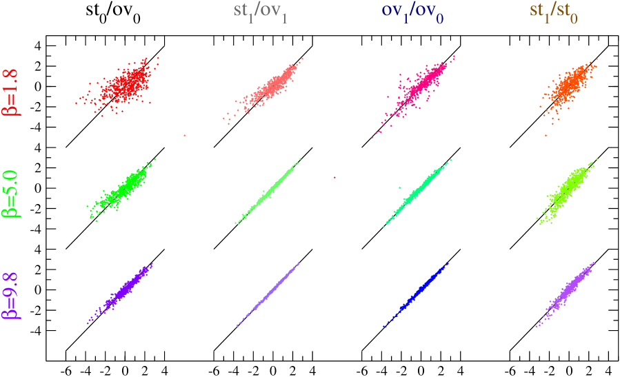
Figure 19: Log-log plot of the rooted staggered versus the overlap determinant, at fixed physical mass $m/e\!=\!0.1$ and $\beta\!=\!1.8,5.0,9.8$ (from top to bottom), without (leftmost column) and after one step of filtering (second column). In addition, we plot smearing level 1 versus level 0 for the overlap (third) and the rooted staggered determinant (fourth column), which are known to deviate through $O(a^{2})$ effects. Throughout, the black line is the identity, not a fit.

We are in an excellent position to test (47), since we have all eigenvalues with either discretization in a number of lattices with fixed physical volume (see Tab. 2). Introducing

$$S^{\mathrm{ov}}_{m}(U,U^{\prime}) = \;\;\;\;\;\;\,-\log\bigg{(}{\det(D_{m}^{\mathrm{ov}}(U))\over\det(D_{m}^{\mathrm{ov}}(U^{\prime}))}\bigg{)}$$ (48)

$$S^{\mathrm{st}}_{m}(U,U^{\prime}) = -{1\over 2^{d/2}}\log\bigg{(}{\det(D_{m}^{\mathrm{\,st}}(U))\over\det(D_{m}^{\mathrm{\,st}}(U^{\prime}))}\bigg{)}$$ (49)

the goal is to show that the unfiltered ratios differ by cut-off effects only, relation (47) or

$$S_{m}^{\mathrm{ov}}(U,U^{\prime})=S_{m}^{\mathrm{st}}(U,U^{\prime})+O(a^{2})\;.$$ (50)

For this it is sufficient to show that an analogous relation holds among the filtered operators

$$S_{m}^{\mathrm{ov}}(U^{(1)},U^{\prime(1)})=S_{m}^{\mathrm{st}}(U^{(1)},U^{\prime(1)})+O(a^{2})\;,$$ (51)

where the superscript $(1)$ refers to the smearing level $1$, since we already know that the left-hand sides and the right-hand sides of (50, 51) satisfy

$$S_{m}^{\mathrm{ov}}(U,U^{\prime}) = S_{m}^{\mathrm{ov}}(U^{(1)},U^{\prime(1)})+O(a^{2})$$ (52)

$$S_{m}^{\mathrm{st}}\,(U,U^{\prime}) = S_{m}^{\mathrm{st}}\,(U^{(1)},U^{\prime(1)})+O(a^{2})$$ (53)

respectively, because filtering amounts to an $O(a^{2})$ redefinition of the operator.

The leftmost column of Fig. 19 contains scatter plots of the two sides of (50) in a fixed physical volume and at a fixed quark mass $m/e$. Each dot represents a configuration $U$, while $U^{\prime}$ is an artificial background which realizes the ensemble mean (over $U$) of (48, 49). Obviously, the correlation on an arbitrary background $U$ gets tighter and the pertinent slope moves closer to 1 as the lattice spacing decreases. Note that this holds regardless of the topological charge, since our ensembles contain a Gaussian distribution of $q$ at each $\beta$. The second column shows the scatter plots of the two sides of (51), where the correlation is much better than before. Finally, the third and fourth columns contain the scatter plots for the known relations (52) and (53). Qualitatively, they look very similar to the first two columns, and this gives some confidence that (50, 47) might actually hold true. In any case, the interesting news is that the 1-filtered staggered action generates, on a fine enough lattice, a distribution that is closer to the the 1-filtered overlap one, than the latter is to the unfiltered overlap distribution.

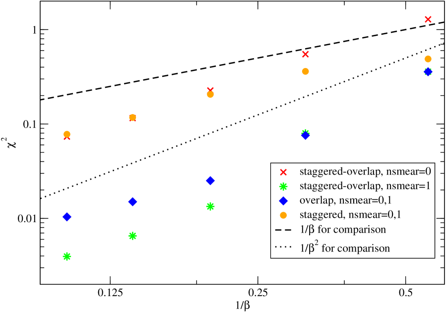
Figure 20: Scaling of $\chi^{2}$, defined in (7), versus $(ae)^{2}$. For the diamonds/bullets it is known that they represent an $O(a^{2})$ redefinition of the operator, for the crosses/stars it is conjectured, because of the striking similarity of the fall-off pattern.

To make the discussion a bit more precise, we introduce a quantity designed to measure the deviation of the correlation from the identity. We use e.g. for the first column

$$\chi^{2} = {1\over\#(U)}\sum_{U}\Big{(}{1\over 2}\log^{\prime}(\det(D^{\mathrm{st}}))-\log^{\prime}(\det(D^{\mathrm{ov}}))\Big{)}^{2}$$ (54)

$$\mathrm{where} \log^{\prime}(\det)=\log(\det)-{1\over\#(U^{\prime})}\sum_{U^{\prime}}\log(\det)$$

and expect that it decreases, in a fixed physical volume, as the lattice spacing gets smaller. Of course, this $\chi^{2}$ is not a physical observable, and one should not expect it to vanish in proportion to $1/\beta\!=\!a^{2}$. Still, the data in Fig. 20 suggest that it falls of – roughly – with a power law in $a$. We tested other $m/e$ which are in the scaling regime with our $\beta$-values and found qualitatively the same behavior. The important point is that there is no obvious difference among the pattern of the four coefficients pertinent to the four columns of Fig. 19. Only the prefactor is different, telling us that the correlation among the two formulations at smearing level 1 is better than the internal overlap correlation between level 0 and 1, and the latter is better than the internal staggered and the staggered-to-overlap correlation without smearing. In other words, the scaling of the coefficient (7) between the overlap and the rooted staggered contribution to the effective action (normalized per physical volume) behaves in the same way as the one for the internal overlap or internal rooted staggered correlation between two smearing levels. Since the latter are known to deviate through $O(a^{2})$ effects, we rate this as strong evidence that also the overlap and rooted staggered determinants differ by $O(a^{2})$ terms, cf. (50, 51) or (47).

8 Summary and discussion

We have attempted scaling tests for dynamical overlap and rooted staggered fermions. The Schwinger model was chosen, because it permits to reach high numerical accuracy while the conceptual issue of square-rooting the staggered determinant remains for ${N_{\!f}}\!=\!1$.

First, we have looked at the scalar condensate at fixed physical quark mass. For $m/e\!>\!0$ the bare staggered and overlap condensates (11, 14) diverge logarithmically in $1/a$. Subtracting the free case without its non-topological zero modes defines a UV and IR safe observable at finite quark mass, and Fig. 9 suggests that it has the same continuum value for staggered and overlap fermions. Hence the analytic value (8) for the condensate in the massless 1-flavor theory can be reproduced with rooted staggered fermions, if the limit $m\!\to\!0$ is taken after letting $a\!\to\!0$. In the overlap formulation the two limits may be interchanged, while in the staggered case the reverse order of limits yields an exact (but incorrect) zero. We consider the non-commutativity phenomenon (35) important, because the Schwinger value (8) reflects the axial anomaly, and the second version indicates that rooted staggered fermions do get the anomaly right, if the continuum limit is taken at finite quark mass.

The second observable has been the topological susceptibility. Both in the continuum and with overlap sea-quarks it vanishes at zero quark mass. Hence $\chi_{\mathrm{top}}^{\mathrm{st}}(m\!=\!0)$ is a pure lattice artefact, and it seems to disappear like $a^{2}$ for an unfiltered (“naive”) staggered Dirac operator, while in a filtered version $O(a^{4}...a^{8})$ terms would numerically dominate over a wide range of couplings. On the other hand, with a finite quark mass, there is no obvious difference among the two formulations, and we have verified that one sees pure $O(a^{2})$ scaling, as expected. Furthermore, the continuum limit of the topological susceptibility with overlap or rooted staggered fermions at fixed physical quark mass is consistent within errors.

Our third observable, the partition function, is a bit more refined, but similar in spirit, to the topological susceptibility. Again we find, at fixed $m/e$, a continuum value, for arbitrary charge $q$, that is consistent within errors. Also the fourth test, a check of the Leutwyler-Smilga sum rule (42) has not revealed any difference of the two formulations in the continuum limit.

The finite temperature heavy-quark force at fixed physical distance has been our fifth test. It is interesting that in the Schwinger model the effects of virtual quark loops are so pronounced and so easy to measure. We find no deviation between the two fermion discretizations, since at filtering level 1 overlap and rooted staggered sea-quarks agree already at the $\beta$-values considered. It is noteworthy that the $a$-dependence of the heavy-quark selfenergy in 2D is entirely different from the one in 4D. As a consequence, a fuzzed heavy-quark action increases the signal-to-noise ratio only on rough lattices in 2D, while this trick helps only on fine lattices in 4D.

Finally, we have investigated the logarithmic determinant ratio of overlap and rooted staggered fermions as a function of the lattice spacing in a fixed physical volume. We find strong evidence that, at a given filtering level, this ratio is constant over the entire configuration space up to $O(a^{2})$ effects, since the pertinent $\chi^{2}$ disappears in the same way as for (52, 53) which are established relations. Of course, this is a numerical argument and not a proof.

In general, we find cut-off effects with dynamical overlap fermions to be smaller than with staggered fermions. Close to the chiral limit, the difference may be dramatic.

As mentioned in the introduction, the conceptual power of a scaling study is one-sided. We might have found an observable where the staggered answer turns out wrong in the continuum, and this would have been sufficient to prove that the rooted staggered action does not represent a legitimate fermion discretization. We have not found such an observable, and the fact that even the condensate in the 1-flavor theory is reproduced correctly (under the right order of limits) lets one feel more sceptical whether such an observable exists. Still, we emphasize that most of our observables involve only sea quarks, and even the finite-mass condensate does not probe the complicated flavor/taste structure that staggered fermions have in the valence sector. Hence, a scaling study focusing on $\pi$ and $\eta^{\prime}$ properties might be worthwhile.

For current dynamical simulations with rooted staggered quarks the implication is two-fold. The good news is that, for any finite sea-quark mass, we find a universal continuum limit in a dynamical theory. This is just numerical evidence and not a proof, but if overlap and staggered quarks would not yield the same result in the continuum, there is no reason why this difference would be particularly small, but non-zero, in the massive Schwinger model. The potentially worrisome observation is the non-commutativity phenomenon (35). This is critical, because in 4D physical results are extracted by fitting the data against predictions from staggered chiral perturbation theory (SXPT) [3], i.e. the limits $a\!\to\!0$ and $m\!\to\!0$ are taken simultaneously. It is not clear to us whether SXPT would accommodate such a non-commutativity (in the full theory), but maybe standard physical observables in 4D QCD with ${N_{\!f}}\!\geq\!2$ are not afflicted with this problem anyways.

Finally, we feel that in future investigations the focus should be on the locality issue mentioned in the introduction. Bunk et al. have shown that the fourth root (in 4D) of $D^{\mathrm{st}}$ is not a local operator [4], but the question is, of course, whether there is any local operator which, when raised to the fourth power, reproduces $D^{\mathrm{st}}$. Obviously, this problem needs to be solved to lend a solid theoretical basis to a mixed action approach as it has been explored in Ref. [36]. Recently, Neuberger has discussed how the operation of taking the fourth root may be cast into a local relativistic framework in 6 dimensions [37]. The question that should be asked, in our opinion, is whether it is really necessary to have a local operator $D$ that satisfies $D^{4}=D^{\mathrm{st}}$ exactly, or whether a version with corrections, say

$$D^{-4}=(D^{\mathrm{st}})^{-1}\!+\!O(a^{2})$$ (55)

for the Green’s functions, would suffice to guarantee that a “hybrid” formulation with a rooted $D^{\mathrm{st}}$ in the determinant and $D$ for the valence quarks yields the correct continuum limit. If so, our Fig. 19 suggest that such a $D$ might be built via the overlap prescription.

Acknowledgments: We thank Tom DeGrand and Victor Laliena for useful correspondence. S.D. wishes to acknowledge discussions with Rainer Sommer, C.H. with Laurent Lellouch and Leonardo Giusti. S.D. was partly supported by DFG in SFB/TR-9, partly by the Swiss NSF. C.H. was supported by EU grant HPMF-CT-2001-01468.

References

- [1]
- [2] C.T.H. Davies et al. [HPQCD Collaboration], Phys. Rev. Lett. 92, 022001 (2004) [hep-lat/0304004].
- [3] C. Aubin et al. [MILC Collaboration], hep-lat/0407028.
- [4] B. Bunk, M. Della Morte, K. Jansen and F. Knechtli, Nucl. Phys. B 697, 343 (2004) [hep-lat/0403022].
- [5] A. Hart and E. Muller, hep-lat/0406030.
- [6] C. Aubin and C. Bernard, Phys. Rev. D 68, 034014 (2003) [hep-lat/0304014]. C. Aubin and C. Bernard, Phys. Rev. D 68, 074011 (2003) [hep-lat/0306026]. S.R. Sharpe and R.S. van de Water, hep-lat/0409018.
- [7] D.H. Adams, Phys. Rev. Lett. 92, 162002 (2004) [hep-lat/0312025]. D.H. Adams, hep-lat/0409013.
- [8] S. Dürr and C. Hoelbling, Phys. Rev. D 69, 034503 (2004) [hep-lat/0311002] and hep-lat/0408039.
- [9] S. Dürr, C. Hoelbling and U. Wenger, Phys. Rev. D 70, 094502 (2004) [hep-lat/0406027] and hep-lat/0409108.
- [10] E. Follana, A. Hart and C.T.H. Davies [HPQCD Collaboration], Phys. Rev. Lett. 93, 241601 (2004) [hep-lat/0406010].
- [11] K.Y. Wong and R.M. Woloshyn, hep-lat/0407003. K.Y. Wong and R.M. Woloshyn, hep-lat/0412001.
- [12] R. Narayanan and H. Neuberger, Nucl. Phys. B 412, 574 (1994) [hep-lat/9307006]. R. Narayanan and H. Neuberger, Nucl. Phys. B 443, 305 (1995) [hep-th/9411108]. H. Neuberger, Phys. Lett. B 417, 141 (1998) [hep-lat/9707022]. H. Neuberger, Phys. Lett. B 427, 353 (1998) [hep-lat/9801031].
- [13] P.H. Ginsparg and K.G. Wilson, Phys. Rev. D 25, 2649 (1982).
- [14] M. Lüscher, Phys. Lett. B 428, 342 (1998) [hep-lat/9802011].
- [15] P. Hernandez, K. Jansen and M. Lüscher, Nucl. Phys. B 552, 363 (1999) [hep-lat/9808010].
- [16] T. Blum et al., Phys. Rev. D 55, 1133 (1997) [hep-lat/9609036]. K. Orginos, D. Toussaint and R.L. Sugar [MILC Collaboration], Phys. Rev. D 60, 054503 (1999) [hep-lat/9903032].
- [17] G.P. Lepage, Phys. Rev. D 59, 074502 (1999) [hep-lat/9809157].
- [18] T. DeGrand [MILC collaboration], Phys. Rev. D 63, 034503 (2001) [hep-lat/0007046]. T. DeGrand, A. Hasenfratz and T.G. Kovacs, Phys. Rev. D 67, 054501 (2003) [hep-lat/0211006].
- [19] J.S. Schwinger, Phys. Rev. 128, 2425 (1962).
- [20] I. Sachs and A. Wipf, Helv. Phys. Acta 65, 652 (1992).
- [21] A. Smilga and J.J.M. Verbaarschot, Phys. Rev. D 54, 1087 (1996) [hep-ph/9511471].
- [22] N.D. Mermin and H. Wagner, Phys. Rev. Lett. 17, 1133 (1966). P.C. Hohenberg, Phys. Rev. 158, 383 (1967). S.R. Coleman, Commun. Math. Phys. 31, 259 (1973).
- [23] C.B. Lang and T.K. Pany, Nucl. Phys. B 513, 645 (1998) [hep-lat/9707024].
- [24] P. Hasenfratz, V. Laliena and F. Niedermayer, Phys. Lett. B 427, 125 (1998) [hep-lat/9801021].
- [25] R. Narayanan, H. Neuberger and P. Vranas, Nucl. Phys. Proc. Suppl. 47, 596 (1996) [hep-lat/9509046]. R. Narayanan, H. Neuberger and P. Vranas, Phys. Lett. B 353, 507 (1995) [hep-lat/9503013]. F. Farchioni, I. Hip and C.B. Lang, Phys. Lett. B 443, 214 (1998) [hep-lat/9809016]. F. Farchioni, I. Hip, C.B. Lang and M. Wohlgenannt, Nucl. Phys. B 549, 364 (1999) [hep-lat/9812018]. S. Chandrasekharan, Phys. Rev. D 59, 094502 (1999) [hep-lat/9810007]. J.E. Kiskis and R. Narayanan, Phys. Rev. D 62, 054501 (2000) [hep-lat/0001026]. L. Giusti, C. Hoelbling and C. Rebbi, Phys. Rev. D 64, 054501 (2001) [hep-lat/0101015].
- [26] E. Marinari, G. Parisi and C. Rebbi, Nucl. Phys. B 190, 734 (1981). J. Polonyi and H.W. Wyld, Phys. Rev. Lett. 51, 2257 (1983), Erratum-ibid. 52, 401 (1984). T. Burkitt, Nucl. Phys. B 220, 401 (1983). A.N. Burkitt and R.D. Kenway, Phys. Lett. B 131, 429 (1983). S.R. Carson and R.D. Kenway, Annals Phys. 166, 364 (1986). M. Grady, Phys. Rev. D 35, 1961 (1987). V. Azcoiti, G. Di Carlo, A. Galante, A.F. Grillo and V. Laliena, Phys. Rev. D 50, 6994 (1994) [hep-lat/9401032]. P. de Forcrand, J.E. Hetrick, T. Takaishi and A.J. van der Sijs, Nucl. Phys. Proc. Suppl. 63, 679 (1998) [hep-lat/9709104].
- [27] Y. Hosotani, hep-th/9703153.
- [28] C. Adam, Phys. Lett. B 440, 117 (1998) [hep-th/9806211].
- [29] H. Leutwyler and A. Smilga, Phys. Rev. D 46, 5607 (1992).
- [30] G. Colangelo and S. Dürr, Eur. Phys. J. C 33, 543 (2004) [hep-lat/0311023].
- [31] K. Ogawa and S. Hashimoto, hep-lat/0409103.
- [32] G.P. Lepage, Nucl. Phys. Proc. Suppl. 26, 45 (1992).
- [33] M. Della Morte et al. [ALPHA Collaboration], Phys. Lett. B 581, 93 (2004) [hep-lat/0307021]. S. Dürr, hep-lat/0409141. M. Della Morte, F. Knechtli, A. Shindler, R. Sommer, to appear.
- [34] E. Eichten and B. Hill, Phys. Lett. B 234, 511 (1990).
- [35] C. Bernard, hep-lat/0412030.
- [36] K.C. Bowler, B. Joo, R.D. Kenway, C.M. Maynard and R.J. Tweedie [UKQCD Collaboration], hep-lat/0411005.
- [37] H. Neuberger, hep-lat/0409144.
- [38] F. Maresca and M. Peardon, hep-lat/0411029.
- [39] D.H. Adams, hep-lat/0411030.
- [40] Y. Shamir, hep-lat/0412014.