DESY 04-217

HU-EP-04-64

MS-TP-04-31

Bicocca-FT-04-16

SFB/CPP-04-59

March 3, 2024

Computation of the strong coupling in QCD with two dynamical flavours

We present a non-perturbative computation of the running of the coupling $\alpha_{\rm s}$ in QCD with two flavours of dynamical fermions in the Schrödinger functional scheme. We improve our previous results by a reliable continuum extrapolation. The $\Lambda$-parameter characterizing the high-energy running is related to the value of the coupling at low energy in the continuum limit. An estimate of $\Lambda r_{0}$ is given using large-volume data with lattice spacings $a$ from $0.07\,\rm fm$ to $0.1\,\rm fm$. It translates into $\Lambda_{\rm\overline{MS\kern-0.35002pt}\kern 0.35002pt}^{(2)}=245(16)(16)\,{\rm MeV}$ [assuming $r_{0}=0.5\,{\rm fm}$]. The last step still has to be improved to reduce the uncertainty.

Keywords: lattice QCD, strong coupling constant

1 Introduction

The QCD sector of the Standard Model of elementary particles constitutes a renormalizable quantum field theory. After determining one mass parameter for each quark species and the strong coupling constant (at some reference energy) which fixes the interaction strength, QCD is believed – and so-far found – to predict all phenomena where only strong interactions are relevant. Due to asymptotic freedom, this programme could be successfully implemented for processes with energies $E\gg 1\,{\rm GeV}$ by using perturbation theory to evaluate QCD. A recent report on such determinations of the coupling implied by a multitude of experiments is found in [?].

At smaller energy the lattice formulation together with the tool of numerical simulation is used to systematically extract predictions of the theory. Here the free parameters are typically determined by a sufficient number of particle masses or matrix elements associated with low energies, and then for instance the remaining hadron spectrum becomes a prediction. See [?] for a recent reference on such large scale simulations.

While this almost looks like two theories having disjoint domains of applicability, we really view QCD as one theory for all scales. Then the adjustable parameters mentioned above are not independent but half of them should in fact be redundant or, in other words, predictable. The ALPHA Collaboration is pursuing the long-term programme of computing the perturbative parameters in the theory matched with Nature at hadronic energies. Here a non-perturbative multi-scale problem has to be mastered: hadronic and perturbative energies have to be covered and kept remote from inevitable infrared and ultraviolet cutoffs. To nevertheless gain good control over systematic errors in such a calculation, a special strategy had to be developed; it will be reviewed in the next section.

As done for many other applications of lattice QCD, also our collaboration has recently set out to overcome the quenched approximation and include vacuum fluctuations due to the two most important light quark flavours. In this article we publish detailed results on the energy dependence of a non-perturbative coupling from hadronic to perturbative energies and thereby connect the two regimes of QCD. This connection has been broken into two parts. It is first established with reference to a scale $L_{\rm max}$ in the hadronic sector that is not yet directly physical but rather technically convenient within our non-perturbative renormalization scheme. This part is, however, a universal continuum result and represents what is mainly reported here. In a second step, which does not anymore involve large physical scale ratios, one number relating our intermediate result to physics, like for instance $L_{\rm max}F_{\pi}$, has to be computed. Here we can cite in this publication only a first estimate and not yet a systematic continuum extrapolation, which is left as a future task.

Earlier milestones of our programme consisted of the formulation of the finite-size scaling technique [?], its adaptation to QCD [?,?], check of universality [?] and the complete numerical execution of all steps in the quenched approximation [?,?,?]. A shorter account of the present study with a subset of the data was published in [?].

We would like to mention that beside our finite-volume technique there are also efforts to compute the coupling and quark masses in a more direct “one-lattice” approach. Some recent references with unquenched results include [?,?,?]. Since it is not possible to accommodate all scales involved on one lattice in a satisfactory fashion, in these works a perturbative connection is established between the bare coupling associated with the lattice cutoff scale $a$ and a renormalized coupling at high energy in a continuum scheme such as $\overline{\rm MS}$. In our view, this step represents the main weakness of the method. Series in the non-universal bare coupling are usually worse behaved than renormalized perturbation theory. There are techniques to improve this (tadpole improvement, boosted perturbation theory) which, in cases where a non-perturbative check is possible, sometimes help more and sometimes help less. Thus it is not easy to verify that one uses this perturbation theory in a regime where it is accurate and to quote realistic errors on this step. On the other hand, this approach is much easier to carry through and typically yields approximate results before an application of our strategy is available.

2 Strategy

A non-perturbative renormalization of QCD addresses the question how the high-energy regime, where perturbation theory has been successfully applied in many cases, is related to the observed hadrons and their interactions at small energies. This relation involves large scale separations and thus is difficult to study by numerical simulation. Naively, it would require simulations with a cutoff $a^{-1}$ much larger than the largest energy scale, combined with a large system size $L$, much larger than the Compton wavelength of the pion. In summary this would mean

$$a^{-1}\gg\mu_{\text{perturbative}}\gg\mu_{\text{hadronic}}\gg L^{-1}\,,$$ (2.1)

to avoid discretization and finite-size errors. This clearly corresponds to – with the current computing power – inaccessibly large lattices.

Our method to overcome these problems has been developed in [?,?,?,?,?,?,?]; pedagogical introductions can be found in [?,?]. The key concept is an intermediate finite-volume renormalization scheme, in which the scale evolution of the coupling (and the quark masses) can be computed recursively from low to very high energies. At sufficiently high energies, the scale evolution is verified to match with perturbation theory and there the $\Lambda$-parameter is determined.

2.1 Renormalization

Any physical quantity $P$ should be independent of the renormalization scale $\mu$. This is expressed by the Callan-Symanzik equation [?,?]

$$\left\{\mu\frac{\partial}{\partial\mu}+\beta(\bar{g})\frac{\partial}{\partial\bar{g}}+\tau(\bar{g})\kern 1.0pt\overline{\kern-1.0ptm\kern-1.0pt}\kern 1.0pt\frac{\partial}{\partial\kern 1.0pt\overline{\kern-1.0ptm\kern-1.0pt}\kern 1.0pt}\right\}P=0\,.$$ (2.2)

Here, the $\beta$-function is given by

$$\beta(\bar{g})=\mu\frac{\partial\bar{g}(\mu)}{\partial\mu}\,.$$ (2.3)

Hence, once the coupling has been defined non-perturbatively for all scales (see section 2.2), also the $\beta$-function is defined beyond perturbation theory. For weak couplings or high energies only, the $\beta$-function can be asymptotically expanded as

$$\beta(\bar{g})=-\bar{g}^{3}\left(b_{0}+b_{1}\bar{g}^{2}+b_{2}\bar{g}^{4}+\ldots\right)\,.$$ (2.4)

In the following we only consider mass independent renormalization schemes [?], in which the renormalization conditions are imposed at zero quark mass. Particular examples are the Schrödinger functional scheme described below, and the ${\rm\overline{MS\kern-0.50003pt}\kern 0.50003pt}$ scheme. If in two such schemes the couplings can be mutually expanded as Taylor series of each other (once they are small enough),

$$\bar{g}^{\prime\,2}=\bar{g}^{2}\left(1+C_{g}^{(1)}\bar{g}^{2}+\ldots\right)\,,$$ (2.5)

then the 1- and 2-loop coefficients $b_{0}$ and $b_{1}$ in (2.4) are universal,

$$b_{0} = \frac{1}{(4\pi)^{2}}\left(11-\frac{2}{3}N_{\rm f}\right)\,,$$ (2.6)

$$b_{1} = \frac{1}{(4\pi)^{4}}\left(102-\frac{38}{3}N_{\rm f}\right)\,,$$ (2.7)

while the higher-order coefficients depend on the choice of the coupling. Starting from the 3-loop coefficient in the ${\rm\overline{MS\kern-0.50003pt}\kern 0.50003pt}$ scheme [?] and its conversion to the minimal subtraction scheme of lattice regularization [?,?,?,?], the 3-loop coefficient in the Schrödinger functional scheme (with all the parameters as specified below)

$$b_{2}=\left(0.483(7)-0.275(5)N_{\rm f}+0.0361(5)N_{\rm f}^{2}-0.00175(1)N_{\rm f}^{3}\right)/(4\pi)^{3}$$ (2.8)

could be obtained in [?].

Now, a special exact solution of the Callan-Symanzik equation (2.2) is the renormalization group invariant $\Lambda$-parameter,

$$\Lambda=\mu\left(b_{0}\bar{g}^{2}(\mu)\right)^{-b_{1}/(2b_{0}^{2})}{\rm e}^{\,-1/(2b_{0}\bar{g}^{2}(\mu))}\exp\left\{-\int_{0}^{\bar{g}(\mu)}\!dx\left[\frac{1}{\beta(x)}+\frac{1}{b_{0}x^{3}}-\frac{b_{1}}{b_{0}^{2}x}\right]\right\}\,.$$ (2.9)

$\Lambda$ is scale independent but renormalization scheme dependent. The transition to other mass independent schemes is accomplished exactly by a 1-loop calculation. If in another scheme the coupling is given through (2.5) with both $\bar{g}^{\prime}$ and $\bar{g}$ taken at the same $\mu$, the $\Lambda$-parameters are related by

$$\Lambda^{\prime}=\Lambda\,{\rm e}^{\,C_{g}^{(1)}/(2b_{0})}\,.$$ (2.10)

In particular, the transition from the Schrödinger functional scheme with two dynamical flavours to the ${\rm\overline{MS\kern-0.50003pt}\kern 0.50003pt}$ scheme of dimensional regularization is provided through [?]

$$\Lambda_{\rm\overline{MS\kern-0.35002pt}\kern 0.35002pt}^{(2)}=2.382035(3)\Lambda^{(2)}\,.$$ (2.11)

2.2 Schrödinger functional

Since we want to connect the perturbative regime of QCD with the non-perturbative hadronic regime, we have to employ a non-perturbative definition of the coupling. Furthermore, the definition of the coupling should be practical. This means that one has to be able to evaluate it on the lattice with a small error, that cutoff effects are reasonably small and that its perturbative expansion to 2-loop order is computable with a reasonable effort. In principle there is a large freedom for the choice of the coupling, however, it turns out that the conditions above are hard to fulfill simultaneously.

To this end we consider the Schrödinger functional, which is the propagation amplitude for going from some field configuration at the time $x_{0}=0$ to another field configuration at the time $x_{0}=T$. Here the space-time is a hyper-cubic Euclidean lattice with discretization length $a$ and volume $T\times L^{3}$. We choose $T=L$ so that $L$ is the only remaining external scale in the continuum limit $a\rightarrow 0$ of the massless theory.

The SU(3) gauge fields $U$ are defined on the links of the lattice, while the fermion fields are defined on the lattice sites. The partition function of this system is given by

$$Z=e^{-\Gamma}=\int_{T\times L^{3}}\!{\rm D}[U,\psi,\overline{\psi}]\ e^{-S[U,\psi,\overline{\psi}]}\,.$$ (2.12)

Here, the action is the sum $S[U,\psi,\overline{\psi}]=S_{\rm g}[U]+S_{\rm f}[U,\psi,\overline{\psi}]$ of the ${\rm O}(a)$ improved plaquette action

$$S_{\rm g}[U]=\frac{1}{g_{0}^{2}}\sum_{p}w(p)\,\hbox{tr}\,(1-U(p))$$ (2.13)

and the fermionic action

$$S_{\rm f}[U,\psi,\overline{\psi}]=\sum_{x}\overline{\psi}(x)(D+m_{0})\psi(x)$$ (2.14)

for two degenerate flavours implicit in $\psi$. For the special boundary conditions considered below, the weight factor $w(p)$ is the boundary improvement term $c_{\rm t}$ [?] for time-like plaquettes at the boundary and one in all other cases. The value of $c_{\rm t}$ has become available to 2-loop order in perturbation theory [?] in the course of this work. Thus some of our data sets use the 1-loop value of $c_{\rm t}$, hence our simulations adopt two different actions. Because of universality we expect them to yield the same continuum limits for our observables.

The ${\rm O}(a)$ improved Wilson Dirac operator $D$ includes the Sheikholeslami-Wohlert term [?] multiplied with the improvement coefficient $c_{\rm sw}$ that has been determined with non-perturbative precision in [?], and a boundary improvement term that is multiplied by the coefficient $\tilde{c}_{\rm t}$, which is known to 1-loop order. For details and notation we refer to [?,?].

The boundary conditions in the space directions are periodic for the gauge fields and periodic up to a global phase $\theta$ for the fermion fields. The value of $\theta$ was optimized at 1-loop order of perturbation theory [?]. It turns out that a value close to $\theta=\pi/5$ leads to a significantly smaller condition number of the fermion matrix than other values of $\theta$ and thus to a smaller computational cost. Benchmarks in the relevant parameter range for our project have shown this too, and therefore we adopt the choice $\theta=\pi/5$ in this work.

In the time direction, Dirichlet boundary conditions are imposed at $x_{0}=0$ and $x_{0}=T$. The quark fields at the boundaries are given by the Grassmann valued fields $\rho,\bar{\rho}$ at $x_{0}=0$ and $\rho^{\prime},\bar{\rho}^{\prime}$ at $x_{0}=T$, respectively. They are used as sources that are set to zero after differentiation. The gauge fields at the boundaries are chosen such that a constant colour-electric background field, which is the unique (up to gauge transformations) configuration of least action, is generated in our space-time [?]. This is achieved by the diagonal colour matrices specified in ref. [?], parametrized by two dimensionless real parameters $\eta$ and $\nu$.

A renormalized coupling $\bar{g}^{2}$ may then be defined by differentiating the effective action $\Gamma$ at the boundary point “A” of [?] that corresponds to the choice $\eta=\nu=0$,

$$\frac{\partial\Gamma}{\partial\eta}\bigg{|}_{\eta=\nu=0}=\frac{k}{\bar{g}^{2}}\,.$$ (2.15)

The normalization $k$ is chosen such that the tree-level value of $\bar{g}^{2}$ equals $g_{0}^{2}$ for all values of the lattice spacing. The boundary point “A” and especially the value $\nu=0$ are used, since the statistical error of the coupling turns out to be small for this choice. For general values of $\nu$ we find another renormalized quantity $\bar{v}$,

$$\frac{\partial\Gamma}{\partial\eta}\bigg{|}_{\eta=0}=k\left\{\frac{1}{\bar{g}^{2}}-\nu\bar{v}\right\}\,,$$ (2.16)

that we have investigated as well to study the effects of dynamical fermions.

The renormalized coupling depends on the system size, the lattice spacing $a$ and on the quark mass. The bare quark mass $m_{0}$ is additively renormalized on the lattice because chiral symmetry is broken for Wilson fermions [?]. Thus we define the bare mass by the PCAC relation that relates the axial current $A^{a}_{\mu}(x)=\overline{\psi}(x)\frac{\tau^{a}}{2}\gamma_{\mu}\gamma_{5}\psi(x)$ to the pseudoscalar density $P^{a}(x)=\overline{\psi}(x)\frac{\tau^{a}}{2}\gamma_{5}\psi(x)$. Using the matrix elements $f_{\rm A}$ and $f_{\rm P}$ of $A^{a}_{\mu}$ and $P^{a}$, respectively (cf. [?]), the ${\rm O}(a)$ improved PCAC mass is defined as

$$m(x_{0})=\frac{\frac{1}{2}(\partial_{0}+\partial_{0}^{\star})f_{\rm A}(x_{0})+c_{\rm A}a\partial_{0}^{\star}\partial_{0}f_{\rm P}(x_{0})}{2f_{\rm P}(x_{0})}\,.$$ (2.17)

We have used 1-loop perturbation theory for $c_{\rm A}$ [?].

To fix all the details of our scheme, we define the bare current mass through

$$m=\left\{\begin{array}[]{ll}m(T/2)\,,&\mbox{if $T/a$ is even,}\\ \left[m((T-a)/2)+m((T+a)/2)\right]/2\,,&\mbox{if $T/a$ is odd.}\end{array}\right.$$ (2.18)

This mass is tuned to zero,

$$m(g_{0},m_{0},L/a)=0\,,$$ (2.19)

so that we have a massless renormalization scheme, in which the only remaining external scale in the continuum limit is the system size $L$.

2.3 Computational Strategy

In the last section we have defined the Schrödinger functional coupling $\bar{g}^{2}$. This finite-volume coupling runs with $\mu=1/L$ and – assuming monotonicity – there is a one-to-one relation between the value of the coupling and the system size $L$ or energy scale $\mu$. In an abuse of notation we will from now on write $\bar{g}^{2}(L)$ instead of $\bar{g}^{2}(1/L)$.

Our goal is to calculate the scale evolution of the strong coupling and the $\Lambda$-parameter of QCD in terms of a low-energy scale. We start the computation by choosing a value $u$ for the renormalized coupling (which implicitly determines $L$) and by choosing a lattice resolution $L/a$. The theory can then be renormalized by tuning the bare parameters $\beta=6/g_{0}^{2}$ and $\kappa=1/(8+2am_{0})$ such that

$$\bar{g}^{2}(L)=u\quad\text{and}\quad m=0\,.$$ (2.20)

Now we simulate a lattice with twice the linear size at the same bare parameters, that means at the same value of the lattice spacing, and thus with the physical extent $2L$, corresponding to a new renormalized coupling $u^{\prime}=\bar{g}^{2}(2L)$. This determines the scale evolution of the renormalized coupling. It can be expressed through the lattice step scaling function

$$\left.\Sigma(u,a/L)=\bar{g}^{2}(2L)\right|_{\bar{g}^{2}(L)=u\,,\,m=0}\,,$$ (2.21)

which is the key observable we compute. Finally, we obtain the step scaling function

$$\sigma(u)=\lim_{a/L\rightarrow 0}\Sigma(u,a/L)$$ (2.22)

in the continuum limit by repeating these three steps with finer and finer lattice resolutions. This algorithm is iterated for a sequence of values for $u$ to get the functional form of $\sigma(u)$.

For small values of $u$ the step scaling function $\sigma(u)$ can be expanded in renormalized perturbation theory,

$$\sigma(u)=u+s_{0}u^{2}+s_{1}u^{3}+\ldots\,,$$ (2.23)

with the coefficients

$$s_{0} = 2\ b_{0}\ln 2\,,$$ (2.24)

$$s_{1} = (2\ b_{0}\ln 2)^{2}+2\ b_{1}\ln 2\,,$$ (2.25)

$$s_{2} = (2\ b_{0}\ln 2)^{3}+10\ b_{0}\ b_{1}(\ln 2)^{2}+2\ b_{2}\ln 2\,.$$ (2.26)

The step scaling function $\sigma(u)$ can be interpreted as an integrated discrete $\beta$-function. Indeed, by using equation (2.3) we get

$$\beta\left(\sqrt{\sigma(u)}\right)=\beta\left(\sqrt{u}\right)\,\sqrt{\frac{u}{\sigma(u)}}\,\sigma^{\prime}(u)$$ (2.27)

for the $\beta$-function, which allows to calculate it recursively once the step scaling function $\sigma(u)$ is known.

To arrive at our main result, that is the $\Lambda$-parameter in terms of a low-energy scale, we solve the equation

$$\sigma\left(\bar{g}^{2}(L/2)\right)=\bar{g}^{2}(L)$$ (2.28)

recursively for $\bar{g}^{2}(L/2)$. We start this recursion at a maximal value $u_{\rm max}=\bar{g}^{2}(L_{\rm max})$ of the coupling. The value of $u_{\rm max}$ is chosen such that the associated scale $L_{\rm max}$ is a scale in the hadronic regime of QCD. Following the recursion (2.28) to larger and larger energies, we obtain the values for

$$u_{i}=\bar{g}^{2}(2^{-i}L_{\rm max})\,,\quad i=0,\ldots,n\,,\quad u_{0}=u_{\rm max}\,.$$ (2.29)

We perform $n=7$ or $n=8$ steps of this recursion and can in this way cover a scale separation of a factor 100 to 250. Eventually, for sufficiently large energies, perturbation theory can safely be applied. Then we use (2.9) with $\mu=2^{n}/L_{\rm max}$ and with the $\beta$-function truncated at 3-loop order, (2.6)–(2.8). The final result for $\Lambda L_{\rm max}$ in the Schrödinger functional scheme can be converted to the ${\rm\overline{MS\kern-0.50003pt}\kern 0.50003pt}$ scheme with (2.11). We also check the admissibility of employing perturbation theory by studying the variation of our final result with respect to the number of non-perturbative steps $n$ in the scale evolution of the strong coupling.

2.4 Discretization effects

The influence of the underlying space-time lattice on the evolution of the coupling can be estimated perturbatively [?], by generalizing Symanzik’s discussion [?,?,?] to the present case. Close to the continuum limit we expect that the relative deviation

$$\delta(u,a/L)=\frac{\Sigma(u,a/L)-\sigma(u)}{\sigma(u)}=\delta_{1}(a/L)u+\delta_{2}(a/L)u^{2}+\ldots$$ (2.30)

of the lattice step scaling function from its continuum limit converges to zero with a rate roughly proportional to $a/L$. More precisely, since the action is ${\rm O}(a)$ improved, we expect

$$\delta_{1}(a/L) \sim \left(d_{0,1}+d_{1,1}\ln\frac{a}{L}\right)\left(\frac{a}{L}\right)^{2}+\ldots\,,$$ (2.31)

$$\delta_{2}(a/L) \sim e_{0,2}\frac{a}{L}+\left(d_{0,2}+d_{1,2}\ln\frac{a}{L}+d_{2,2}\left(\ln\frac{a}{L}\right)^{2}\right)\left(\frac{a}{L}\right)^{2}+\ldots$$ (2.32)

for the 1-loop value of $c_{\rm t}$ and the same form with $e_{0,2}=0$ for the 2-loop value of $c_{\rm t}$. Note that the tree-level discretization effects vanish exactly, since we normalize the coupling such that its perturbative expansion starts with $g_{0}^{2}$ for all values of the lattice spacing.

The coefficients $\delta_{1}$ and $\delta_{2}$ are collected in table 1 for the resolutions needed in this work.

$L/a$	$\delta_{1}$	$\delta_{2}^{c_{\rm t}=\text{1-loop}}$	$\delta_{2}^{c_{\rm t}=\text{2-loop}}$
4	$-0.0103$	0.0063	$-0.00007$
5	$-0.0065$	0.0049	$-0.00019$
6	$-0.0042$	0.0038	$-0.00041$
8	$-0.0021$	0.0029	$-0.00030$

Table 1: Discretization error of the step scaling function.

An expanded version of this table can be found in [?]. The entries in the last column are very small. For larger values of $L/a$ than shown in the table, $\delta_{2}^{c_{\rm t}=\text{2-loop}}$ decreases as expected. Since $\delta_{2}^{c_{\rm t}=\text{1-loop}}$ is of the order $a/L$, it is no surprise that it is much larger than $\delta_{2}^{c_{\rm t}=\text{2-loop}}$. In fact, it is of the same size as $\delta_{1}$, for which the linear term in $a/L$ is absent.

The largest coupling at which the step scaling function has been computed with the 1-loop value of $c_{\rm t}$ is $u=1.7319$. With the 2-loop value of $c_{\rm t}$, this is $u=3.334$. Table 1 suggests that the step scaling function is only mildly affected by discretization effects. This will be demonstrated by our numerical results in section 4.

We cancel the known perturbative cutoff effects for the respective actions by using

$$\Sigma^{(2)}(u,a/L)=\frac{\Sigma(u,a/L)}{1+\delta_{1}(a/L)u+\delta_{2}(a/L)u^{2}}$$ (2.33)

in the analysis of our Monte Carlo data. The perturbative estimate of the relative cutoff effects behaves as $(a/L)\times u^{3}$ close to the continuum limit.

2.5 Matching to a hadronic scheme

As described so far, our computational strategy yields $\Lambda L_{\rm max}$, with $L_{\rm max}$ defined by the value of the coupling itself. Since the latter is not experimentally measurable, it remains to relate $L_{\rm max}$ to a hadronic scale. Here, the natural choice is the pion decay constant $F_{\pi}$, since chiral perturbation theory provides an analytic understanding of the pion dynamics [?,?], which is expected to help to control the extrapolations to the physical quark mass [?] as well as to infinite volume [?].

A computation of $L_{\rm max}F_{\pi}$ requires the knowledge of $f(\tilde{g}_{0}^{2})=aF_{\pi}$ (at a quark mass where $m_{\pi}/F_{\pi}$ takes its experimental value) and $l(g_{0}^{2})=L_{\rm max}/a$, where $\bar{g}^{2}(L_{\rm max})=u_{\rm max}$. We remind the reader that $\bar{g}^{2}$ is defined at vanishing quark mass. The difference between the improved bare coupling $\tilde{g}_{0}$ [?] and $g_{0}$ is proportional to the light quark mass and can safely be neglected for physical values of the light quark mass. We therefore replace $\tilde{g}_{0}\approx g_{0}$ in the following. The value of $u_{\rm max}$ is restricted to be in the range covered by the computation of the scale dependence of the coupling and, for lattice spacings accessible in large-volume simulations, $l(g_{0}^{2})$ should be sufficiently large. With both functions, $l$ and $f$, defined for the same discretization, one finally wants to evaluate

$$\left.L_{\rm max}\,F_{\pi}\right|_{\rm continuum}=\lim_{f\to 0}l(g_{0}^{2})f(g_{0}^{2})\,.$$ (2.34)

Unfortunately, the results available in the literature [?,?] for $f(g_{0}^{2})$ with our action [?] suffer from an uncertainty in the renormalization of the axial current, which has not yet been performed non-perturbatively. Also the O$(a)$ improvement of the current is known only perturbatively and it is not obvious that quark masses have been reached where chiral perturbation theory is applicable.

At present, we thus prefer to relate $L_{\rm max}$ to the frequently used hadronic radius $r_{0}$, which, according to phenomenological considerations, has a value of around $0.5\,{\rm fm}$ [?] and which has also been the reference scale in the zero-flavour theory, i.e. the quenched approximation [?]. Note that in a calculation in this approximation agreement was found (within its 3% precision) between $F_{\rm K}r_{0}$ and the product of the experimental number for $F_{\rm K}$ times $0.5\,$fm [?]. Below, we thus evaluate $L_{\rm max}/r_{0}=l(g_{0}^{2})/\rho(g_{0}^{2})$ where $\rho(g_{0}^{2})=r_{0}/a$ and translate to physical units via $r_{0}=0.5\,{\rm fm}$.

3 Details of the numerical simulation and analysis

In addition to the piece present in the pure gauge theory [?], the central observable, $\partial\Gamma/\partial\eta$, receives a contribution due to the quark determinant. We describe its numerical evaluation by a stochastic estimator in appendix A. Also detailed tables with simulation results are deferred to an appendix (B).

3.1 Tuning

With a number of tuning runs we determine the bare parameters $\beta$ and $\kappa$ such that eq. (2.20) is valid. Fulfilling the condition $m(L)=0$ precisely would require a fine tuning of the hopping parameter $\kappa$. However, the uncertainty in $\Sigma$ owing to a small mismatch of $m$ can be estimated perturbatively. To this end we compute the derivative of $\Sigma$ with respect to $z=mL$,

$$\left.\frac{\partial}{\partial z}\bar{g}^{2}(2L)\right|_{\bar{g}^{2}(L)=u\,,\,m(L)=z/L}=\Phi(a/L)u^{2}+\ldots\,.$$ (3.35)

It turns out that $\Phi$ is a slowly varying function of $a/L$. Thus, for our purpose it suffices to approximate it by its universal part,

$$\Phi(0)=-\frac{N_{\rm f}}{4\pi}\left.\frac{\partial}{\partial z}c_{1,1}(z)\right|_{z=0}=0.00957N_{\rm f}\,,$$ (3.36)

where $c_{1,1}(z)$ has been taken from [?]. The typical precision in Monte Carlo simulations is $\Delta(\bar{g}^{-2})=\bar{g}^{-4}\Delta(\bar{g}^{2})=0.003$, as can be seen from the tables 10 and 11 in appendix B. This means that an additional error of $0.001\times u^{2}$ due to a slight mismatch of the mass $m(L)$ is tolerable. Then it suffices to require

$$am<0.1\frac{a}{L}\frac{1}{N_{\rm f}}\,.$$ (3.37)

The tables 10 and 11 in appendix B show that we have reached this precision in our simulations.

Analogously, we stop the fine tuning of $\beta$ if $\bar{g}^{2}(L)=u$ well within the errors. Then we can correct for a small mismatch owing to $\bar{g}^{2}(L)=\tilde{u}\neq u$ by using

$$\Sigma(u,a/L)=\Sigma(\tilde{u},a/L)+\Sigma^{\prime}(u,a/L)\times(u-\tilde{u})\,,$$ (3.38)

with the perturbative estimate

$$\Sigma^{\prime}(u,a/L)\equiv\frac{\partial\Sigma(u,a/L)}{\partial u}\approx\frac{\partial\sigma(u)}{\partial u}\approx 1+2s_{0}u+3s_{1}u^{2}+4s_{2}u^{3}$$ (3.39)

for the derivative of the step scaling function $\Sigma$. This correction is always smaller than the statistical error of the step scaling function.

Similarly, we convert the statistical error on $u$ into an additional error of $\Sigma$,

$$\Delta\left(\Sigma(u)\right)\approx\Sigma^{\prime}(u,a/L)\times\Delta(u)\approx(1+2s_{0}u+\ldots)\times\Delta(u)\,.$$ (3.40)

This additional error is always much smaller than the error of $\bar{g}^{2}(2L)$, to which it is added in quadrature.

In some cases we have stopped the fine tuning of $\beta$ and $\kappa$ after a number of runs and interpolated the results such that exactly the target coupling and mass zero with the errors as shown in the tables 10 and 11 were obtained.

The step scaling function $\Sigma(u,a/L)$ and its partner with the perturbative cutoff effects being divided out, $\Sigma^{(2)}(u,a/L)$ (cf. (2.33)), are listed in table 2.

$u$	$L/a$	$\Sigma(u,a/L)$	$\Sigma^{(2)}(u,a/L)$	$u$	$L/a$	$\Sigma(u,a/L)$	$\Sigma^{(2)}(u,a/L)$
0.9793	4	1.0643(35)	1.0686(35)	1.5031	4	1.7204(56)	1.7477(57)
	5	1.0720(40)	1.0738(41)		5	1.737(11)	1.755(11)
	6	1.0802(46)	1.0807(46)		6	1.730(13)	1.743(13)
	8	1.0736(59)	1.0729(59)		8	1.723(16)	1.730(16)
1.1814	4	1.3154(55)	1.3199(56)	2.0142	4	2.481(18)	2.535(18)
	5	1.3296(61)	1.3307(61)		5	2.438(20)	2.473(20)
	6	1.3253(70)	1.3249(70)		6	2.507(27)	2.533(28)
	8	1.3342(71)	1.3323(71)		8	2.475(35)	2.489(35)
1.5031	4	1.7310(61)	1.7332(61)	2.4792	4	3.251(28)	3.338(29)
	5	1.756(12)	1.754(12)		5	3.336(52)	3.394(53)
	6	1.745(12)	1.741(12)		6	3.156(57)	3.198(58)
					8	3.326(52)	3.351(53)
1.7319	4	2.0583(76)	2.0562(76)	3.334	4	5.588(54)	5.791(56)
	5	2.083(21)	2.076(21)		5	5.43(11)	5.56(11)
	6	2.058(20)	2.049(20)		6	5.641(99)	5.75(10)
					8	5.48(13)	5.53(13)

Table 2: Step scaling functions $\Sigma$ and $\Sigma^{(2)}$. The left hand side of the table contains the data with the 1-loop value of $c_{\rm t}$, while the data with $c_{\rm t}=\text{2-loop}$ are shown on the right.

3.2 Parameters

Our choice of parameters is displayed in table 10 and table 11 in appendix B. The parameters shown are the results of a careful application of the tuning procedure explained in the last section. The tables reveal that the condition $\bar{g}^{2}(L)=u$ is fulfilled to a good precision. The remaining deviations and the errors are then propagated into an additional error for $\Sigma(u)$, as described above.

3.3 Simulation costs and proper sampling of the configuration space

Most of our results have been produced with the hybrid Monte Carlo algorithm (HMC) [?], the polynomial hybrid Monte Carlo (PHMC) in the version proposed in [?,?] and for some of the $L/a=16$ runs the hybrid Monte Carlo algorithm generalized to two pseudofermion fields (HMC 2 pf) [?,?].

We measure the cost of our simulations with the quantity

$$M_{\rm cost} = {\rm(update\;time\;in\;seconds\;on\;machine\;M})$$

$$\times\,{\rm{(error\;of}}\;1/\bar{g}^{2})^{2}\times(4a/T)(4a/L)^{3}\,.$$

In [?] the cost of a subset of the simulations discussed here (essentially up to $L/a=12$ and $\bar{g}^{2}\approx 2.5$) has been analyzed. A typical value for HMC at $L/a=10$ and $\bar{g}^{2}\approx 2.5$ is $M_{\rm cost}\approx 3.5$, with respect to one board of APEmille [?]. To give an idea about the increase of the cost for the $L/a=16$ simulations, we collect results from two different runs at the coupling $\bar{g}^{2}\approx 2.5$ in table 3. We compute the autocorrelation time $\tau_{\rm int}$ in units of trajectories in the way suggested in [?].

algorithm	step size	$\tau_{\rm int}$	$t_{\rm update}/[\,s\,]$	$\bar{g}^{2}$	$N_{\rm traj}$	$M_{\rm cost}$
HMC	$0.0625$	$3.6(3)$	$380$	$2.46(5)$	$4800$	$6.9(6)$
HMC 2 pf	$0.111$	$4.6(4)$	$262$	$2.55(5)$	$5900$	$5.6(5)$

Table 3: Cost estimates for two $L/a=16$ runs; $t_{\rm update}/[\,s\,]$ is the time in seconds needed for one trajectory of length 1. The reference machine is an APEmille board.

Related to the issue of estimating the autocorrelation time is always the question whether the algorithm samples the entire relevant configuration space efficiently. If this is not the case, autocorrelation times may be largely underestimated and even systematically wrong results may be obtained. We now discuss two at least rough checks that our simulations do not suffer from such problems.

1. To investigate the contributions to the coupling from sectors of configuration space with non-trivial topology, we have performed a set of simulations at the coupling $\bar{g}^{2}\approx 2.5$ with $L/a=8,12$. The topological charge $Q(U)$ is determined through a cooling procedure. Since sampling different topological sectors might be algorithmically very difficult, we have employed the PHMC algorithm, whose flexibility can be exploited to enhance the transition rate among different sectors (at the price of increasing the fluctuations of the reweighting factor), and checked the results to be independent of the polynomial approximation used.

Starting from a hot, random configuration, several of the independent replica were in a non-trivial topological sector. For these replica the smallest eigenvalue of $D^{2}$ (even-odd preconditioned) turns out to be one order of magnitude smaller than typical values in the topologically trivial sectors. After ${\rm O}(100)$ trajectories for $L/a=8$, respectively O(1000) trajectories for $L/a=12$, all the replica have zero topological charge and transitions to sectors with $Q(U)\neq 0$ have not been observed in additional ${\rm O}(10^{4})$ trajectories.

From this we conclude that the PHMC algorithm can tunnel between different topological sectors, but for large $L/a$ the transition rate is very small. In addition, the weight of the non-trivial sectors is too small for them to occur in a practical simulation at all (all tunnellings went to $Q(U)=0$ and none in the reverse direction). Their weight in the path integral is negligible. These statements have been checked for $L/a=8,12$, and it appears safe to assume their validity also for larger $L/a$. Therefore, we decided to always start from a cold configuration, especially for the $L/a=16$ simulations, to avoid thermalization problems.

2. For the two largest couplings discussed here the distribution of $\partial S/\partial\eta$ shows long tails toward negative values. The same effect was also observed in the computation of the Schrödinger functional coupling in pure SU(3) gauge theory [?]. We have related this tail to secondary local minima of the action [?] by measuring on cooled configurations the pure gauge contribution to the action $S_{\rm g}^{\rm cool}$ and to the coupling $\partial S_{\rm g}^{\rm cool}/\partial\eta$. This leads to metastabilities as shown for an $L/a=16$ simulation with $\bar{g}^{2}\approx 3.3$ in figure 1.

Figure 1: Monte Carlo histories of $S_{\rm g}^{\rm cool}$ and $\partial S_{\rm g}^{\rm cool}/\partial\eta$ from two independent replica (solid and dotted lines) in a simulation of a $16^{4}$ lattice at $\bar{g}^{2}\approx 3.3$.

The upper panel is the Monte Carlo history ($t_{\rm MD}$ is the Monte Carlo time in units of molecular dynamics trajectories) of the gauge part of the action after cooling for two independent replica. The lower panel shows the history of $\partial S_{\rm g}^{\rm cool}/\partial\eta$ for the same two replica. The correlation between metastable states and small (even negative) values of $\partial S_{\rm g}^{\rm cool}/\partial\eta$ appears evident in this case. The action $S_{\rm g}^{\rm cool}$ for the metastability in the figure is consistent with the value for a secondary solution of the field equations [?], given our choice for the boundary fields. Numerical evidence suggests that this solution is a local minimum.

In order to estimate the weight of these contributions in our expectation values properly, we have enhanced their occurrence through a modified sampling similar to [?], adding to the HMC effective action a term

$$\left.\gamma\,{{\partial S_{\rm g}}\over{\partial\eta}}\right|_{\eta=0}+{{1}\over{w_{\gamma}}}\,(\gamma-\gamma_{0})^{2}\,,$$ (3.42)

where $\gamma_{0}$ and $w_{\gamma}$ are fixed to suitable (positive) values, while $\gamma$ is a dynamical variable. The expectation values in the original ensemble are then obtained by reweighting. By some deterministic cooling procedure with a fixed number of cooling steps we now define a quantity $q$ whose value is 1 for metastable configurations, and 0 otherwise, such that $\delta_{q1}+\delta_{q0}\equiv 1$. For an arbitrary observable $O$ we have an exact identity

$$\langle O\rangle = \langle\delta_{q1}O\rangle+\langle\delta_{q0}O\rangle$$

$$= \langle\delta_{q1}O\rangle+\langle O\rangle_{\bar{1}}(1-\langle\delta_{q1}\rangle)\,,$$

with $\langle O\rangle_{\bar{1}}=\langle\delta_{q0}O\rangle/\langle\delta_{q0}\rangle$. If the main contribution to $\langle O\rangle$ comes from the configurations with $q=0$, a precise estimate of $\langle O\rangle$ just requires a precise estimate of $\langle O\rangle_{\bar{1}}$, which can be obtained by an algorithm that samples only the $q=0$ sector, together with rough estimates of $\langle\delta_{q1}\rangle$ and $\langle\delta_{q1}O\rangle$ that can be obtained by the modified sampling.

At $\bar{g}^{2}\approx 3.3$ we get $\langle\delta_{q1}\rangle=0.3(2)\%$, independent of $L/a=8,12$ within the error. The effect of metastable states on the coupling is $0.10(2)\%$. At the coupling $\bar{g}^{2}\approx 5.5$ the occurrence of metastable states is much more frequent, as expected, and we get $\langle\delta_{q1}\rangle=5(1)\%$. At the same time their sampling is much easier already in the original ensemble, using either the PHMC or the HMC algorithm. In fact, we have repeated the $L/a=12$ simulation for $\bar{g}^{2}\approx 5.5$ using PHMC for the ordinary ensemble (without (3.42)) as in [?], but measuring in addition the occurrence of metastable states. This turned out to be around $6\%$, and for $\bar{g}^{2}$ we have obtained a result fully consistent with the number in [?].

In summary, we can be confident that topologically non-trivial sectors are irrelevant for our observables with our choice of parameters and at the present level of precision. In contrast, there are secondary minima in the action, which are visible as metastable states in the Monte Carlo sequence. They are relevant starting at $\bar{g}^{2}\approx 3$ and have been taken into account efficiently by deviating from naive importance sampling and combining two different properly chosen ensembles.

4 Results

4.1 The strong coupling

In figure 2 we show the approach of the step scaling function $\Sigma^{(2)}(u,a/L)$ to the continuum limit. The cutoff effects are small. Actually, all the data are compatible with constants. If we use simple fits to constants, the combined $\chi^{2}$ per degree of freedom for all the eight continuum extrapolations is about 1.4 regardless of the number of lattices included in the fit. Even the points at $L/a=4$ are compatible with a constant continuum extrapolation. One possible strategy for the continuum extrapolation is thus a fit to a constant that uses the lattices with $L/a=6,8$.

In this fit to constants we exclude the two coarsest lattices since there is always the danger of including systematic cutoff effects into the results coming from the lattices with large $a/L$. Therefore, we have also investigated two alternative fit procedures. The first and most conservative one (denoted as “global fit” in the tables) is a combined continuum extrapolation of all the data sets, but excluding $L/a=4$. Here we use the two-parameter ansatz

$$\Sigma^{(2)}(u,a/L)=\sigma(u)+\rho^{X}\,u^{4}\,(a/L)^{2}\,,\quad X\in\{\text{1-loop},\text{2-loop}\}\,,$$ (4.44)

for the lattice artifacts, where the coefficients $\rho^{X}$ are understood to be associated to the data with the 1-loop and the 2-loop value of $c_{\rm t}$, respectively. This fit results in $\rho^{\text{1-loop}}=0.08(13)$ and $\rho^{\text{2-loop}}=0.01(4)$, quantifying that lattice artifacts are not detectable in our data. Moreover we have studied a mixed fit procedure, using a fit to constants for the lattices with $L/a=6,8$ for the 2-loop improved data sets and the global fit ansatz (4.44), which includes a slope for the cutoff effects, for the 1-loop improved data sets.

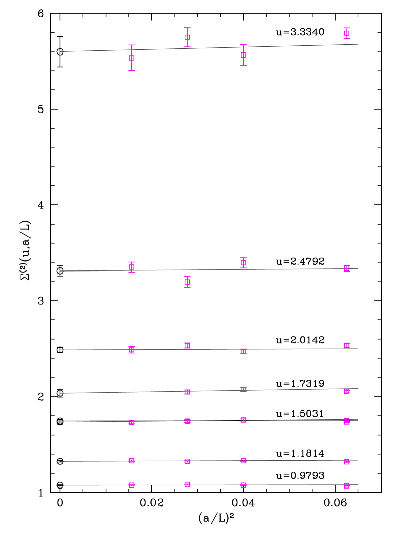
Figure 2: Continuum extrapolation of the step scaling function.

These different fits are performed to investigate the uncertainties in the continuum results. All our plots refer to the most conservative of these three fit procedures, which leaves both $\rho^{\text{1-loop}}$ and $\rho^{\text{2-loop}}$ unconstrained.

$u$	$\sigma(u)$
	global fit	fit to constants	mixed fit
0.9793	1.0736(44)	1.0778(36)	1.0736(44)
1.1814	1.3246(81)	1.3285(50)	1.3246(81)
1.5031	1.733(23)	1.741(12)	1.733(23)
1.7319	2.037(41)	2.049(20)	2.037(41)
1.5031	1.7440(97)	1.738(10)	1.738(10)
2.0142	2.488(26)	2.516(22)	2.516(22)
2.4792	3.311(52)	3.281(39)	3.281(39)
3.3340	5.60(16)	5.670(80)	5.670(80)

Table 4: Continuum limit of the step scaling function.

The results of the continuum limit extrapolation of the step scaling function $\Sigma^{(2)}(u,a/L)$ are recorded in table 4. At $u=1.5031$ we have two sets of data, one of which was produced with the 1-loop value and the other with the 2-loop value of $c_{\rm t}$. Both continuum results agree well within their errors, which is an independent check of our extrapolation procedures.

We interpolate the values of table 4 by a polynomial of degree 6 in $u$, the first coefficients up to $u^{3}$ being fixed by 2-loop perturbation theory, cf. (2.23). This interpolation is depicted in figure 3.

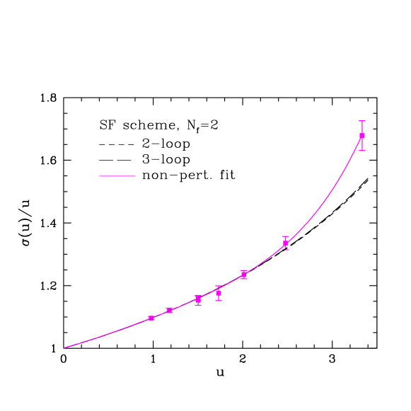
Figure 3: Step scaling function $\sigma(u)$. The dashed lines show the perturbative results from the integration of the 2-loop and 3-loop $\beta$-function, respectively.

For small values of $u<2$, the step scaling function is well described by perturbation theory. Actually, the perturbative lines shown in this plot are the solution of

$$-2\ln 2=\int_{u}^{\sigma(u)}\!\frac{dx}{\sqrt{x}\ \beta(\sqrt{x})}$$ (4.45)

for $\sigma(u)$ using the 2-loop and the 3-loop $\beta$-function. Looking at the comparison of successive perturbative approximations to the non-perturbative results, it appears likely that higher orders would not improve the agreement at the largest coupling. Rather we appear to have reached a value for the coupling, where the perturbative expansion has broken down. In fact, already in section 3.3 we have discussed the indications that fluctuations around a secondary minimum of the action are important at this value of the coupling. Such a mechanism may represent one possible source of non-perturbative effects.

We adopt the parametrized form of the step scaling function to compute the $\Lambda$-parameter. To this end we start a recursion with a maximal coupling $u_{\text{max}}=\bar{g}^{2}(L_{\text{max}})$. For $u_{\rm max}=5.5$, the recursive step (2.28) is solved numerically to get the couplings $u_{i}$, corresponding to the energy scales $\mu=2^{i}/L_{\rm max}$, that are quoted in table 5. We then insert these couplings into eq. (2.9) for the $\Lambda$-parameter, using there the 3-loop $\beta$-function.

global fit			constant fit, $L/a=6,8$		mixed cont. extrap.
$i$	$u_{i}$	$-\ln(\Lambda L_{\text{max}})$	$u_{i}$	$-\ln(\Lambda L_{\text{max}})$	$u_{i}$	$-\ln(\Lambda L_{\text{max}})$
0	5.5	0.957	5.5	0.957	5.5	0.957
1	3.306(40)	1.071(25)	3.291(18)	1.081(12)	3.291(19)	1.081(12)
2	2.482(31)	1.093(37)	2.479(20)	1.096(23)	2.471(20)	1.106(24)
3	2.010(27)	1.093(48)	2.009(19)	1.096(35)	2.003(19)	1.106(35)
4	1.695(22)	1.089(57)	1.691(16)	1.099(43)	1.690(17)	1.103(44)
5	1.468(18)	1.087(65)	1.462(14)	1.109(49)	1.464(15)	1.100(52)
6	1.296(16)	1.086(73)	1.288(12)	1.122(55)	1.292(14)	1.100(63)
7	1.160(14)	1.086(82)	1.151(11)	1.138(62)	1.157(13)	1.101(74)
8	1.050(13)	1.088(93)	1.041(10)	1.155(70)	1.048(13)	1.103(87)

Table 5: Recursive computation of the $\Lambda$-parameter starting at $u_{0}=u_{\text{max}}=5.5$.

This gives the results in the third column of table 5. Employing the 2-loop $\beta$-function leads to results that are larger by roughly $0.02$. The table shows that for $u<2$ the $\Lambda$-parameter barely moves within its error bars. To be conservative, we use the global fit result and quote

$$-\ln(\Lambda L_{\text{max}})=1.09(7)\quad\text{at}\quad u_{\text{max}}=5.5$$ (4.46)

as our final result, if the hadronic scale $L_{\text{max}}$ is defined through $u_{\text{max}}=5.5$.

We have in addition computed the $\Lambda$-parameter as a function of $u_{\text{max}}$ in the interval $u_{\text{max}}=3.0\ldots 5.5$. The results can be parametrized as

$$-\ln(\Lambda L_{\text{max}})=\frac{1}{2b_{0}\,u_{\text{max}}}+\frac{b_{1}}{2b_{0}^{2}}\ln(b_{0}\,u_{\text{max}})-0.1612+0.0379\,u_{\text{max}}\,.$$ (4.47)

This parametrization is motivated by (2.9) and represents the central values of our data with a precision better than one permille. The absolute error of $-\ln(\Lambda L_{\text{max}})$ that we quote for all the values of $u_{\text{max}}$ is $0.07$. This means that we have calculated the $\Lambda$-parameter in units of $L_{\text{max}}$ with a precision of seven percent.

The running of the Schrödinger functional coupling $\alpha(\mu)=\bar{g}^{2}(1/\mu)/(4\pi)$ as a function of $\mu/\Lambda$ is displayed in figure 4.

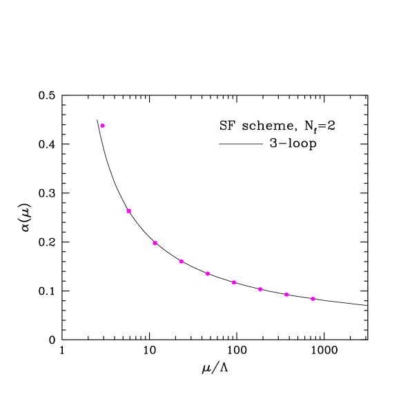
Figure 4: Running of the strong coupling in the Schrödinger functional scheme.

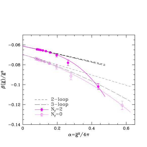
Figure 5: Non-perturbative $\beta$-function in the Schrödinger functional scheme.

The points refer to the entries of the second column of table 5. The symbol size is larger than their error. The difference between the perturbative and the non-perturbative running of the coupling looks small in this plot. However, if we had used perturbation theory only to evolve the coupling over the range considered here, the $\Lambda$-parameter would have been overestimated by up to $14\%$, depending on $u_{\text{max}}$. This corresponds to an extra error of $3\%$ for the coupling in the range where its value is close to 0.12, corresponding to the physical value of $\alpha_{\rm\overline{MS\kern-0.35002pt}\kern 0.35002pt}$ at $M_{\rm Z}$. Needless to add, this error could of course not even be quantified without non-perturbative information.

Furthermore, our non-perturbative coupling was designed to have a good perturbative expansion, since we rely on the 3-loop $\beta$-function in the (high-energy part of the) computation of the $\Lambda$-parameter. With our computation we have shown that for the Schrödinger functional coupling there is an overlapping region where both, perturbative and non-perturbative methods apply. In no way is this to be interpreted as a general statement about QCD observables or couplings at certain energies.

In figure 5 we show the non-perturbative $\beta$-function in the Schrödinger functional scheme, together with the 2-loop and the 3-loop perturbation theory. It has been obtained recursively from (2.27). The derivative of the step scaling function needed there has been calculated from the polynomial interpolating $\sigma(u)$ (see continuous line in figure 3). The non-perturbative data are fitted with two parameters beyond the 2-loop $\beta$-function. The plot again shows an overlapping region in $\bar{g}$, where the perturbative and the non-perturbative $\beta$-functions agree well with each other. For $\alpha>0.2$, however, perturbation theory is no longer valid. Furthermore, the plot shows the difference between $N_{\rm f}=0$ and $N_{\rm f}=2$. Already the leading coefficient $b_{0}$ of the $\beta$-function depends on the number of flavours, and this is nicely reflected in the figure.

4.2 Computation of $\bar{v}$ as a function of the strong coupling

The difference between the quenched approximation and the two-flavour theory is also apparent in the renormalized quantity $\bar{v}$ defined in (2.16). As a function of the coupling $u$ we write (at zero quark mass)

$$\bar{v}=\omega(u)=\lim_{a/L\rightarrow 0}\Omega(u,a/L)\,.$$ (4.48)

In perturbation theory, $\Omega$ is known to 2-loop order,

$$\Omega(u,a/L)=(v_{1}+v_{2}u)\left(1+\epsilon_{1}(a/L)+\epsilon_{2}(a/L)u\right)+{\rm O}(u^{2})\,.$$ (4.49)

Here [?,?,?],

$$v_{1} = 0.0694603(1)+0.0245370(1)N_{\rm f}\,,$$ (4.50)

$$v_{2} = -0.001364(14)-0.000101(17)N_{\rm f}-0.0003362(30)N_{\rm f}^{2}\,,$$ (4.51)

and the perturbative cutoff effects are listed in table 6. Note that the tree-level coefficient of $\bar{v}$ vanishes exactly because of the definition of the couplings. The perturbative results indicate a large effect for going from the zero- to the two-flavour theory.

		$N_{\rm f}=0$			$N_{\rm f}=2$
$L/a$		$\epsilon_{1}(a/L)$	$\epsilon_{2}(a/L)$		$\epsilon_{1}(a/L)$	$\epsilon_{2}(a/L)$
4		0.1880609(17)	$-0.02020(24)$		0.3044344(25)	$0$.	$03725(43)$
5		0.1085045(16)	$-0.01347(22)$		0.1822083(22)	$0$.	$01255(39)$
6		0.0677292(15)	$-0.00910(22)$		0.1114033(21)	$0$.	$00325(36)$
7		0.0460993(15)	$-0.00660(21)$		0.0727865(20)	$-0$.	$00047(35)$
8		0.0335967(15)	$-0.00513(21)$		0.0502340(20)	$-0$.	$00130(34)$
10		0.0203927(15)	$-0.00357(21)$		0.0280832(19)	$-0$.	$00118(34)$
12		0.0138002(15)	$-0.00273(20)$		0.0181305(19)	$-0$.	$00091(33)$
14		0.0099904(15)	$-0.00219(20)$		0.0127946(19)	$-0$.	$00074(33)$
16		0.0075781(15)	$-0.00181(20)$		0.0095635(19)	$-0$.	$00064(33)$
20		0.0047983(14)	$-0.00133(20)$		0.0059634(19)	$-0$.	$00050(33)$
24		0.0033132(14)	$-0.00103(20)$		0.0040873(19)	$-0$.	$00040(33)$

Table 6: Cutoff effects of $\bar{v}$ in perturbation theory.

The first step in the analysis is to project $\bar{v}$ on zero mass. To this end we have obtained the crude estimate $\partial\bar{v}/\partial(am)\approx-0.15(4)$ at constant $u$ from the matching runs at the smallest coupling and with $L/a=4$. We use it also at the other couplings. After this projection, the perturbative cutoff effects are eliminated (similarly to (2.33)) by replacing $\Omega$ by

$$\Omega^{(2)}(u,a/L)=\frac{\Omega(u,a/L)}{1+\epsilon_{1}(a/L)+\epsilon_{2}(a/L)u}$$ (4.52)

in the analysis. In contrast to the coupling, this correction is substantial and the resulting continuum extrapolation is much smoother [?].

Then we project $\Omega^{(2)}(u,a/L)$ on some reference couplings in the range $u=0.9793\ldots 5.5$, using a numerical estimate for the slope. In principle, we would have to propagate the error of $u=\bar{g}^{2}$ into an extra error of $\Omega^{(2)}(u,a/L)$. However, it turns out, both from perturbation theory and from the non-perturbative fits later, that the variation of $\bar{v}$ with $u$ is so small that this extra error can safely be neglected.

We make an ansatz linear in $(a/L)^{2}$ for the continuum extrapolation. The data for the two different actions are extrapolated separately and the continuum results are then averaged according to their weight. The data at $L/a=4,5$ are left out.

The results are displayed in figure 6 together with $\bar{v}$ at $N_{\rm f}=0$ from ref. [?]. The comparison shows that $\bar{v}$ increases by almost a factor two when going from the quenched approximation to $N_{\rm f}=2$.

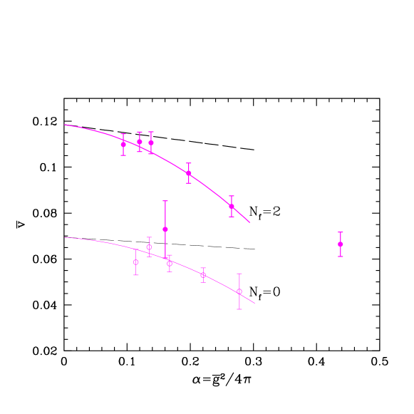
Figure 6: $\bar{v}$ as a function of the strong coupling $\alpha$. The dashed lines show the 2-loop perturbation theory while the solid lines are non-perturbative fits for $\alpha<0.3$ including an additional $\alpha^{2}$-term.

4.3 Evaluation of $\Lambda r_{0}$

For the O($a$) improved action [?] used in our computations, the low-energy scale $r_{0}$ has been calculated at $\beta\equiv 6/g_{0}^{2}=5.2$ (or $a\approx 0.1\,$fm) by two groups [?,?]. Recently, these large-volume $N_{\rm f}=2$ simulations of QCD have been extended to smaller values of the lattice spacing, namely $5.2\leq\beta\leq 5.4$ [?]. In order to obtain $\Lambda r_{0}$ and to study its dependence on the lattice spacing, we here use results for $r_{0}/a$ of [?] at $\beta=5.2,5.29,5.4$ and compare also to the numbers resulting from $r_{0}/a$ of [?].

			$c_{\rm t}$=1-loop	$c_{\rm t}$=2-loop
$\beta$	$\kappa$	$L/a$	$\bar{g}^{2}(L)$
5.20	0.13600	4	3.32(2)	3.65(3)
5.20	0.13600	6	4.31(4)	4.61(4)
5.29	0.13641	4	3.184(16)	3.394(17)
5.29	0.13641	6	4.059(32)	4.279(37)
5.29	0.13641	8	5.34(8)	5.65(9)
5.40	0.13669	4	3.016(20)	3.188(24)
5.40	0.13669	6	3.708(31)	3.861(34)
5.40	0.13669	8	4.704(59)	4.747(63)

Table 7: Simulation results for $\bar{g}^{2}(L)$ at low $\beta$. The hopping parameters $\kappa$ are set to the critical ones ($\kappa_{\rm c}$) of [?].

First, we obtain the renormalized coupling on lattices with extent $L/a=4,6,8$ at the three chosen values of $\beta$. It is listed in table 7. The hopping parameters $\kappa$ are taken from [?]. They correspond to roughly massless pions and thus massless quarks. We checked that reasonable changes of $\kappa$, e.g. requiring eq. (2.19), affect our analysis only to a negligible amount. We then set the improvement coefficient $c_{\rm t}$ to its 2-loop value and obtain $L_{\rm max}/a$ for the three values of $\beta$ combined with two fixed values $u_{\rm max}\equiv\bar{g}^{2}(L_{\rm max})=3.65$ and $u_{\rm max}=4.61$ by an interpolation of the data in table 7. These values of $L_{\rm max}/a$, which are recorded in table 8, are insensitive to the interpolation formula used.

		$u_{\rm max}=3.65$		$u_{\rm max}=4.61$
$\beta$	$r_{0}/a$	$L_{\rm max}/a$	$\Lambda_{\rm\overline{MS\kern-0.35002pt}\kern 0.35002pt}\,r_{0}$	$L_{\rm max}/a$	$\Lambda_{\rm\overline{MS\kern-0.35002pt}\kern 0.35002pt}\,r_{0}$
5.20	5.45(5)(20)	4.00(6)	0.655(27)	6.00(8)	0.610(25)
5.29	6.01(4)(22)	4.67(6)	0.619(25)	6.57(6)	0.614(24)
5.40	7.01(5)(15)	5.43(9)	0.621(17)	7.73(10)	0.609(16)

Table 8: Low-energy scale $r_{0}$ in the chiral limit and the combination $\Lambda_{\rm\overline{MS\kern-0.28001pt}\kern 0.28001pt}\,r_{0}$ as obtained for two values of $u_{\rm max}=\bar{g}^{2}(L_{\rm max})$.

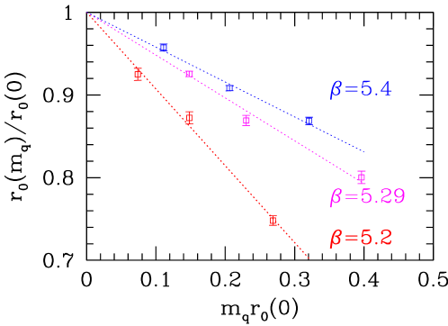
Figure 7: Dependence of $r_{0}$ on the bare quark mass $m_{\rm q}=(1/\kappa-1/\kappa_{\rm c})/2$. Both quantities are rescaled (made dimensionless) by the extrapolated value of $r_{0}$, denoted by $r_{0}(0)$. The uncertainty of this rescaling is not propagated into the errors. For $\kappa_{c}$, we take the values of [?], listed in table 7.

Second, we analyze the raw data for $r_{0}/a$ at finite bare quark masses, $m_{\rm q}$, in order to obtain the value corresponding to massless quarks (the up- and down-quark masses may safely be neglected in this context). At each bare coupling, three different quark masses, corresponding to pion masses between about $500\,{\rm MeV}$ and $1\,{\rm GeV}$, have been simulated in [?]. As seen in figure 7, the radius $r_{0}$ depends approximately linearly on the bare quark mass in this range. The figure also demonstrates that the slope is strongly cutoff dependent; its magnitude decreases quite rapidly as $\beta$ increases (the lattice spacing decreases). This has been noted earlier [?] and reminds us that the study of lattice artifacts is important. On the other hand, we are here not interested in the slope but in $r_{0}$ at zero quark mass. We estimate it by a simple linear extrapolation in $m_{\rm q}$. Since the linear behaviour is not guaranteed to extend all the way to zero quark mass, we include a systematic error of the extrapolation in addition to the statistical one: an uncertainty of half the difference of the last data point and the extrapolated value is added as the second error in table 8. Within the total error, dominated by the systematic one due to the extrapolation, our values of $r_{0}/a$ do agree with those quoted in [?,?,?], where somewhat different ansätze – and in [?] also different data – have been used.

Third, combining eqs. (4.47) and (2.11) with $r_{0}/a$ and $L_{\rm max}/a$ of table 8, one arrives at the columns $\Lambda_{\rm\overline{MS\kern-0.35002pt}\kern 0.35002pt}\,r_{0}$ in that table. Here we have added errors in quadrature, except for the one attributed to eq. (4.47), which is independent of the bare coupling. The resulting $\Lambda_{\rm\overline{MS\kern-0.35002pt}\kern 0.35002pt}\,r_{0}$ are remarkably stable with respect to the change of the lattice spacing and also the choice of $u_{\rm max}$. In particular, for $L_{\rm max}/a>4.5$ all numbers including their errors are covered by the interval $0.58\leq\Lambda_{\rm\overline{MS\kern-0.35002pt}\kern 0.35002pt}\,r_{0}\leq 0.66$ and also the central value obtained with the worst discretization $L_{\rm max}/a=4$ is inside. We thus quote

$$\Lambda_{\rm\overline{MS\kern-0.35002pt}\kern 0.35002pt}^{(2)}\,r_{0}=0.62(4)(4)$$ (4.53)

as our result, the second error deriving from the $7\%$ error on $\Lambda L_{\rm max}$.

We finally mention that we repeated the above analysis also for $c_{\rm t}$ to 1-loop precision and the values $u_{\rm max}=3.32$ and $4.31$ suggested by table 7. The central values for $\Lambda_{\rm\overline{MS\kern-0.35002pt}\kern 0.35002pt}\,r_{0}$ are then up to $15\%$ lower than for $c_{\rm t}$ at 2-loop precision, but this difference shrinks as $L_{\rm max}/a$ grows. At the largest value of $L_{\rm max}/a$, the number for $\Lambda_{\rm\overline{MS\kern-0.35002pt}\kern 0.35002pt}\,r_{0}$ is again fully contained in the range $\Lambda_{\rm\overline{MS\kern-0.35002pt}\kern 0.35002pt}\,r_{0}=0.62(4)$.

5 Conclusions

This non-perturbative QCD computation has required extensive simulations of $N_{\rm f}=2$ QCD with O($a$) improved massless Wilson fermions in finite volume. In our situation, discretization errors turned out to be very small, as seen for example in figure 2 and also in [?]. Although we could achieve the necessary precision only on lattices up to a size $16^{4}$, the smallness of discretization errors allowed to obtain the running of the QCD coupling in the continuum limit and to good accuracy. As in the $N_{\rm f}=0$ (pure gauge) theory, the energy dependence of the coupling in the Schrödinger functional scheme is now known over more than two orders of magnitude in the energy scale. This is the main result of our investigation.

The $N_{\rm f}$-dependence is best illustrated in figure 5, where we also observe excellent agreement with 3-loop perturbation theory for $\alpha\leq 0.2$, while for larger $\alpha$, the non-perturbative $\beta$-function breaks away rapidly from the perturbative approximation. At $\alpha\approx 0.3\ldots 0.4$, a couple of additional higher-order perturbative terms with coefficients of a reasonable size would not be able to come close to the non-perturbative $\beta$-function.

To calibrate the overall energy scale, one fixes a large enough value of the coupling to be in the low-energy region and relates the associated distance, $L_{\rm max}$, to a non-perturbative, large-volume observable. For technical reasons, explained in section 2.5, we have chosen the hadronic radius $r_{0}$, which has an unambiguous definition in terms of the force $F(r)$ between static quarks, via $r_{0}^{2}F(r_{0})=1.65$ [?]. This quantity has also been chosen in the computation of the $\Lambda$-parameter for $N_{\rm f}=0$ [?]. We compare $\Lambda r_{0}$ for various numbers of flavours in table 9.

$N_{\rm f}$	$\Lambda_{\rm\overline{MS\kern-0.35002pt}\kern 0.35002pt}^{(N_{\rm f})}\,r_{0}$	reference	remarks
0	0.60(5)	[?]
2	0.62(4)(4)	this work
4	0.57(8)	[?,?,?]	DIS NNLO & $r_{0}=0.5\,{\rm fm}$
4	0.74(10)	[?]	world average & $r_{0}=0.5\,{\rm fm}$
5	0.54(8)	[?]	world average & $r_{0}=0.5\,{\rm fm}$

Table 9: The QCD $\Lambda$-parameter in units of $r_{0}$. Non-perturbative, purely theoretical determinations for $N_{\rm f}=0,2$ are compared to extractions of $\Lambda$ from high-energy scattering experiments, using high-order perturbation theory combined with the phenomenological estimate $r_{0}\approx 0.5\,{\rm fm}$ [?].

The last two entries in the table represent one and the same world average by S. Bethke of $\alpha$-measurements. They are related by the perturbative matching of the effective theories with $N_{\rm f}=4$ and $N_{\rm f}=5$ massless quarks [?]. While little can be said on the $N_{\rm f}$-dependence of $\Lambda_{\rm\overline{MS\kern-0.35002pt}\kern 0.35002pt}^{(N_{\rm f})}\,r_{0}$ on general grounds, the prediction that there should be a significant drop from $N_{\rm f}=4$ to $N_{\rm f}=5$ depends only on perturbation theory at the scale of the b-quark mass and should thus be reliable. A similar statement for the change from $N_{\rm f}=3$ to $N_{\rm f}=4$ is less certain as it involves physics at and below the mass of the charm quark.

Another relevant issue in the above comparison is that we used $r_{0}\approx 0.5\,{\rm fm}$ to relate the high-energy experiments to our theoretical predictions. Although it appears unlikely that $r_{0}$ differs by 10% from this value, a true error is difficult to estimate until a reliable non-perturbative computation of e.g. $r_{0}F_{\pi}$ has been performed. Indeed, such a computation, or more directly the computation of $L_{\rm max}\times F_{\pi}$ for $N_{\rm f}=2$, is the most urgent next step to be taken in our programme. After that, the effect of the remaining (massive) quarks needs to be estimated.

Keeping the above caveats in mind, we still may convert the $\Lambda$-parameter to physical units and obtain

$$\Lambda_{\rm\overline{MS\kern-0.35002pt}\kern 0.35002pt}^{(2)}=245(16)(16)\,{\rm MeV}\quad\text{[with $r_{0}=0.5\,{\rm fm}$]}\,.$$ (5.54)

Although in this case the four-flavour theory has not yet been reached, it is a very non-trivial test of QCD that the non-perturbative results, which use experimental input at low energies of order $1/r_{0}\approx 400\,{\rm MeV}$, agree roughly with the high-energy, perturbative extractions of $\Lambda$. Unravelling the details in this comparison will still require some work; some of it was just mentioned.

Now, that $\alpha(\mu)$ is known, the tables presented in this work also provide the bare parameters of our lattice action needed in the computation of the energy dependence of the renormalized quark mass and composite operators. These are then readily related to the appropriate renormalization group invariants.

Appendix A Evaluation of $\partial\Gamma/\partial\eta$

Our central observable, eq.(2.15), translates into the expectation value

$$\frac{\partial\Gamma}{\partial\eta}\bigg{|}_{\eta=0}=\left\langle\frac{{\rm d}S}{{\rm d}\eta}\right\rangle=\left\langle\frac{{\rm d}S_{\rm g}}{{\rm d}\eta}\right\rangle+\left\langle\frac{{\rm d}S_{\rm f}^{\rm eff}}{{\rm d}\eta}\right\rangle\,,$$ (A.55)

where the pure gauge part ${\rm d}S_{\rm g}/{\rm d}\eta$ has been discussed in [?] and

$$\frac{{\rm d}S_{\rm f}^{\rm eff}}{{\rm d}\eta}=-N_{\rm f}{\rm Tr}\,Q^{-1}\frac{{\rm d}Q}{{\rm d}\eta}=-N_{\rm f}\,\left\langle\,\varphi^{\dagger}Q^{-1}\frac{{\rm d}Q}{{\rm d}\eta}\varphi\,\right\rangle_{\varphi}\,.$$ (A.56)

Here we have used $S_{\rm f}^{\rm eff}=-N_{\rm f}{\rm Tr}\ln Q$ with $Q=\gamma_{5}(D+m_{0})=Q^{\dagger}$ and $D$ the (one-flavour) Dirac operator including improvement terms. As usual, $S_{\rm f}^{\rm eff}$ is obtained after integrating out the fermion fields and the trace extends over colour and Dirac indices as well as over the space-time points. The last expression in eq. (A.56) represents an average over a complex random field $\varphi(x)$ with the property

$$\langle\varphi^{\ast}_{c\alpha}(x)\varphi_{d\beta}(y)\rangle_{\varphi}=\delta_{cd}\,\delta_{\alpha\beta}\,\delta_{xy}\,,$$ (A.57)

where $c,d$ denote colour indices and $\alpha,\beta$ are Dirac indices. We may finally rewrite ${\rm d}S_{\rm f}^{\rm eff}/{\rm d}\eta$ in the form

$$\frac{{\rm d}S_{\rm f}^{\rm eff}}{{\rm d}\eta} = -N_{\rm f}\,\left\langle\,\sum_{x|x_{0}\in\{a,T-a\}}\frac{1}{2}\,\hbox{tr}\,\,\frac{{\rm d}Q(x,x)}{{\rm d}\eta}\left[\varphi(x)X^{\dagger}(x)+X(x)\varphi^{\dagger}(x)\right]\right\rangle_{\varphi}\,,$$ (A.58)

$$QX=\varphi\,,$$

where we have used the fact that ${\rm d}Q/{\rm d}\eta$ vanishes except for the clover terms, which are diagonal in the coordinate $x$ and contribute only on the time slices $x_{0}=a$ and $x_{0}=T-a$. Now “tr” is over spin and colour only. Eq. (A.58) is in the form used in [?] for the contribution of the clover terms to the pseudofermionic force in the HMC algorithm and is evaluated analogously. Only one solution of the Dirac equation is needed.

Of course, the average over the gauge fields can be interchanged with the one over the field $\varphi$ and one may replace (A.56) by an average over a finite number of fields $\varphi$ drawn from a distribution satisfying (A.57). We found that the fluctuations of such a noisy (unbiased) estimator for ${\rm d}S_{\rm f}^{\rm eff}/{\rm d}\eta$ are small compared to the ones of ${\rm d}S_{\rm g}/{\rm d}\eta$, already when only one field $\varphi$ (from a Gaussian distribution) is used per gauge configuration. This has hence been our method of choice in all simulations.

Appendix B Detailed numerical results

The following tables list detailed parameters and results of our simulations.

$L/a$	$\beta$	$\kappa$	$\bar{g}^{2}$	$\Delta(\bar{g}^{2})$	$\bar{v}$	$\Delta(\bar{v})$	$m$		$\Delta(m)$
$u=0.9793$
4	9.2364	0.1317486	0.9793	0.0007	0.1557	0.0019	$-0$.	$00600$	0.00011
5	9.3884	0.1315391	0.9794	0.0009	0.1322	0.0023	$0$.	$00197$	0.00005
6	9.5000	0.1315322	0.9793	0.0011	0.1266	0.0016	$-0$.	$00014$	0.00003
8	9.7341	0.131305	0.9807	0.0017	0.1177	0.0042	$0$.	$00074$	0.00006
8	9.2364	0.1317486	1.0643	0.0034	0.1244	0.0061	$0$.	$00010$	0.00004
10	9.3884	0.1315391	1.0721	0.0039	0.1151	0.0077	$0$.	$00210$	0.00003
12	9.5000	0.1315322	1.0802	0.0044	0.1227	0.0072	$-0$.	$00091$	0.00002
16	9.7341	0.131305	1.0753	0.0055	0.1047	0.0080	$-0$.	$00008$	0.00003
$u=1.1814$
4	8.2373	0.1327957	1.1814	0.0005	0.1483	0.0016	$0$.	$00100$	0.00011
5	8.3900	0.1325800	1.1807	0.0012	0.1353	0.0018	$-0$.	$00018$	0.00009
6	8.5000	0.1325094	1.1814	0.0015	0.1269	0.0014	$-0$.	$00036$	0.00003
8	8.7223	0.1322907	1.1818	0.0029	0.1141	0.0048	$-0$.	$00115$	0.00004
8	8.2373	0.1327957	1.3154	0.0055	0.1209	0.0061	$0$.	$00020$	0.00005
10	8.3900	0.1325800	1.3287	0.0059	0.1128	0.0070	$0$.	$00097$	0.00007
12	8.5000	0.1325094	1.3253	0.0067	0.1304	0.0068	$-0$.	$00102$	0.00002
16	8.7223	0.1322907	1.3347	0.0061	0.1065	0.0049	$-0$.	$00194$	0.00002
$u=1.5031$
4	7.2103	0.1339411	1.5031	0.0010	0.1437	0.0010	$-0$.	$00074$	0.00010
5	7.3619	0.1339100	1.5044	0.0027	0.1250	0.0031	$0$.	$00052$	0.00010
6	7.5000	0.1338150	1.5031	0.0025	0.1201	0.0024	$-0$.	$00078$	0.00004
8	7.2103	0.1339411	1.7310	0.0059	0.1151	0.0037	$0$.	$00959$	0.00004
10	7.3619	0.1339100	1.7581	0.0113	0.1062	0.0084	$0$.	$00257$	0.00005
12	7.5000	0.1338150	1.7449	0.0119	0.1223	0.0073	$-0$.	$00138$	0.00004
$u=1.7319$
4	6.7251	0.1347424	1.7319	0.0020	0.1378	0.0009	$-0$.	$00181$	0.00013
5	6.8770	0.1346900	1.7333	0.0032	0.1272	0.0025	$-0$.	$00005$	0.00011
6	7.0000	0.1345794	1.7319	0.0034	0.1161	0.0023	$-0$.	$00002$	0.00005
8	6.7251	0.1347424	2.0583	0.0070	0.1008	0.0032	$0$.	$01051$	0.00005
10	6.8770	0.1346900	2.0855	0.0208	0.0934	0.0080	$0$.	$00335$	0.00006
12	7.0000	0.1345794	2.0575	0.0196	0.0833	0.0082	$-0$.	$00049$	0.00006

Table 10: Simulation parameters and results using the 1-loop value for $c_{\rm t}$.

$L/a$	$\beta$	$\kappa$	$\bar{g}^{2}$	$\Delta(\bar{g}^{2})$	$\bar{v}$	$\Delta(\bar{v})$	$m$		$\Delta(m)$
$u=1.5031$
4	7.2811	0.1338383	1.5031	0.0012	0.1434	0.0013	$0$.	$00043$	0.00015
5	7.4137	0.1338750	1.5033	0.0026	0.1310	0.0027	$-0$.	$00083$	0.00009
6	7.5457	0.1337050	1.5031	0.0030	0.1247	0.0031	$0$.	$00072$	0.00008
8	7.7270	0.133488	1.5031	0.0035	0.1219	0.0032	$-0$.	$00084$	0.00003
8	7.2811	0.1338383	1.7204	0.0054	0.1091	0.0037	$0$.	$00928$	0.00004
10	7.4137	0.1338750	1.7372	0.0104	0.1110	0.0063	$0$.	$00109$	0.00004
12	7.5457	0.1337050	1.7305	0.0122	0.0893	0.0079	$-0$.	$00006$	0.00008
16	7.7270	0.133488	1.7231	0.0151	0.1017	0.0092	$-0$.	$00154$	0.00019
$u=2.0142$
4	6.3650	0.1353200	2.0142	0.0024	0.1349	0.0017	$0$.	$00000$	0.00023
5	6.5000	0.1353570	2.0142	0.0044	0.1236	0.0024	$0$.	$00002$	0.00011
6	6.6085	0.1352600	2.0146	0.0056	0.1205	0.0029	$0$.	$00030$	0.00009
8	6.8217	0.134891	2.0142	0.0102	0.0991	0.0045	$0$.	$00049$	0.00007
8	6.3650	0.1353200	2.4814	0.0172	0.1016	0.0049	$0$.	$01318$	0.00008
10	6.5000	0.1353570	2.4383	0.0188	0.0900	0.0050	$0$.	$00367$	0.00005
12	6.6085	0.1352600	2.5077	0.0259	0.1074	0.0069	$0$.	$00013$	0.00004
16	6.8217	0.134891	2.475	0.031	0.0916	0.0076	$-0$.	$00053$	0.00006
$u=2.4792$
4	5.8724	0.1360000	2.4792	0.0034	0.1206	0.0016	$0$.	$00000$	0.00026
5	6.0000	0.1361820	2.4792	0.0073	0.1085	0.0023	$-0$.	$00009$	0.00014
6	6.1355	0.1361050	2.4792	0.0082	0.1025	0.0032	$0$.	$00000$	0.00013
8	6.3229	0.1357673	2.4792	0.0128	0.1015	0.0053	$0$.	$00000$	0.00016
8	5.8724	0.1360000	3.2511	0.0277	0.0859	0.0043	$0$.	$01819$	0.00011
10	6.0000	0.1361820	3.3356	0.0502	0.0796	0.0064	$0$.	$00579$	0.00009
12	6.1355	0.1361050	3.1558	0.0552	0.0801	0.0079	$0$.	$00078$	0.00007
16	6.3229	0.1357673	3.3263	0.0472	0.0806	0.0074	$0$.	$00039$	0.00017
$u=3.3340$
4	5.3574	0.1356400	3.3340	0.0109	0.1087	0.0013	$0$.	$00000$	0.00040
5	5.5000	0.1364220	3.3340	0.0182	0.0965	0.0018	$-0$.	$00004$	0.00017
6	5.6215	0.1366650	3.3263	0.0196	0.0894	0.0031	$0$.	$00051$	0.00018
8	5.8097	0.1366077	3.334	0.019	0.0887	0.0042	$0$.	$00000$	0.00004
8	5.3574	0.1356400	5.588	0.049	0.0576	0.0036	$0$.	$03163$	0.00019
10	5.5000	0.1364220	5.430	0.098	0.0585	0.0048	$0$.	$01126$	0.00012
12	5.6215	0.1366650	5.624	0.089	0.0607	0.0043	$0$.	$00334$	0.00015
16	5.8097	0.1366077	5.4763	0.1236	0.0689	0.0052	$0$.	$00048$	0.00004

Table 11: Simulation parameters and results using the 2-loop value for $c_{\rm t}$.

References

- [1] S. Bethke, Nucl. Phys. Proc. Suppl. 135 (2004) 345, hep-ex/0407021.
- [2] K.I. Ishikawa, plenary talk at LATTICE ’04, Fermilab, Batavia IL, USA, 2004, hep-lat/0410050.
- [3] M. Lüscher, P. Weisz and U. Wolff, Nucl. Phys. B359 (1991) 221.
- [4] M. Lüscher et al., Nucl. Phys. B384 (1992) 168, hep-lat/9207009.
- [5] S. Sint, Nucl. Phys. B451 (1995) 416, hep-lat/9504005.
- [6] ALPHA, G. de Divitiis et al., Nucl. Phys. B437 (1995) 447, hep-lat/9411017.
- [7] ALPHA, S. Capitani et al., Nucl. Phys. B544 (1999) 669, hep-lat/9810063.
- [8] ALPHA, J. Garden et al., Nucl. Phys. B571 (2000) 237, hep-lat/9906013.
- [9] ALPHA, J. Heitger et al., Nucl. Phys. Proc. Suppl. 106 (2002) 859, hep-lat/0110201.
- [10] ALPHA, A. Bode et al., Phys. Lett. B515 (2001) 49, hep-lat/0105003.
- [11] TXL, A. Spitz et al., Phys. Rev. D60 (1999) 074502, hep-lat/9906009.
- [12] QCDSF, M. Göckeler et al., (2004), hep-lat/0409166.
- [13] C. Davies et al., Nucl. Phys. Proc. Suppl. 119 (2003) 595, hep-lat/0209122.
- [14] B. Bunk et al., Nucl. Phys. B697 (2004) 343, hep-lat/0403022.
- [15] M. Lüscher et al., Nucl. Phys. B389 (1993) 247, hep-lat/9207010.
- [16] M. Lüscher et al., Nucl. Phys. B413 (1994) 481, hep-lat/9309005.
- [17] S. Sint, Nucl. Phys. Proc. Suppl. 42 (1995) 835, hep-lat/9411063.
- [18] R. Sommer, Non-perturbative Renormalization of QCD, Lectures given at 36th Internationale Universitätswochen für Kernphysik und Teilchenphysik, Schladming, Austria, 1997, hep-ph/9711243.
- [19] M. Lüscher, Advanced lattice QCD, Lectures given at Les Houches Summer School in Theoretical Physics, Les Houches, France, 1997, hep-lat/9802029.
- [20] C.G. Callan Jr., Phys. Rev. D2 (1970) 1541.
- [21] K. Symanzik, Commun. Math. Phys. 18 (1970) 227.
- [22] S. Weinberg, Phys. Rev. D8 (1973) 3497.
- [23] Y. Frishman, R. Horsley and U. Wolff, Nucl. Phys. B183 (1981) 509.
- [24] O.V. Tarasov, A.A. Vladimirov and A.Y. Zharkov, Phys. Lett. B93 (1980) 429.
- [25] M. Lüscher and P. Weisz, Nucl. Phys. B452 (1995) 213, hep-lat/9504006.
- [26] M. Lüscher and P. Weisz, Nucl. Phys. B452 (1995) 234, hep-lat/9505011.
- [27] B. Allés, A. Feo and H. Panagopoulos, Nucl. Phys. B491 (1997) 498, hep-lat/9609025.
- [28] A. Bode and H. Panagopoulos, Nucl. Phys. B625 (2002) 198, hep-lat/0110211.
- [29] ALPHA, A. Bode, P. Weisz and U. Wolff, Nucl. Phys. B576 (2000) 517, Erratum-ibid. B600 (2001) 453, Erratum-ibid. B608 (2001) 481, hep-lat/9911018.
- [30] S. Sint and R. Sommer, Nucl. Phys. B465 (1996) 71, hep-lat/9508012.
- [31] B. Sheikholeslami and R. Wohlert, Nucl. Phys. B259 (1985) 572.
- [32] ALPHA, K. Jansen and R. Sommer, Nucl. Phys. B530 (1998) 185, hep-lat/9803017.
- [33] M. Lüscher et al., Nucl. Phys. B478 (1996) 365, hep-lat/9605038.
- [34] M. Lüscher and P. Weisz, Nucl. Phys. B479 (1996) 429, hep-lat/9606016.
- [35] K.G. Wilson, Phys. Rev. D10 (1974) 2445.
- [36] K. Symanzik, Some topics in quantum field theory, in Mathematical problems in theoretical physics, eds. R. Schrader et al., Lecture Notes in Physics Vol. 153 (Springer, New York, 1982).
- [37] K. Symanzik, Nucl. Phys. B226 (1983) 187.
- [38] K. Symanzik, Nucl. Phys. B226 (1983) 205.
- [39] B. Gehrmann et al., Nucl. Phys. B612 (2001) 3, hep-lat/0106025.
- [40] S. Weinberg, Physica A96 (1979) 327.
- [41] J. Gasser and H. Leutwyler, Ann. Phys. 158 (1984) 142.
- [42] G. Colangelo, plenary talk at LATTICE ’04, Fermilab, Batavia IL, USA, 2004, hep-lat/0409111.
- [43] UKQCD, A.C. Irving et al., Phys. Lett. B518 (2001) 243, hep-lat/0107023.
- [44] JLQCD, S. Aoki et al., Phys. Rev. D68 (2003) 054502, hep-lat/0212039.
- [45] R. Sommer, Nucl. Phys. B411 (1994) 839, hep-lat/9310022.
- [46] S. Duane et al., Phys. Lett. B195 (1987) 216.
- [47] R. Frezzotti and K. Jansen, Nucl. Phys. B555 (1999) 395, hep-lat/9808011.
- [48] R. Frezzotti and K. Jansen, Nucl. Phys. B555 (1999) 432, hep-lat/9808038.
- [49] M. Hasenbusch, Phys. Lett. B519 (2001) 177, hep-lat/0107019.
- [50] M. Hasenbusch and K. Jansen, Nucl. Phys. B659 (2003) 299, hep-lat/0211042.
- [51] ALPHA, R. Frezzotti et al., Comput. Phys. Commun. 136 (2001) 1, hep-lat/0009027.
- [52] A. Bartoloni et al., Nucl. Phys. Proc. Suppl. 106 (2002) 1043, hep-lat/0110153.
- [53] ALPHA, U. Wolff, Comput. Phys. Commun. 156 (2004) 143, hep-lat/0306017.
- [54] ALPHA, M. Della Morte et al., Nucl. Phys. Proc. Suppl. 119 (2003) 439, hep-lat/0209023.
- [55] A. Bode, to two loop including cutoff effects, unpublished notes, 2001.
- [56] UKQCD, C.R. Allton et al., Phys. Rev. D65 (2002) 054502, hep-lat/0107021.
- [57] QCDSF, M. Göckeler et al., (2004), hep-ph/0409312.
- [58] ALPHA, R. Sommer et al., Nucl. Phys. Proc. Suppl. 129 (2004) 405, hep-lat/0309171.
- [59] J. Blümlein, H. Böttcher and A. Guffanti, (2004), hep-ph/0407089.
- [60] S. Moch, J.A.M. Vermaseren and A. Vogt, Nucl. Phys. B688 (2004) 101, hep-ph/0403192.
- [61] W.L. van Neerven and E.B. Zijlstra, Phys. Lett. B272 (1991) 127.
- [62] W. Bernreuther and W. Wetzel, Nucl. Phys. B197 (1982) 228.
- [63] K. Jansen and C. Liu, Comput. Phys. Commun. 99 (1997) 221, hep-lat/9603008.