DFTT 13/2004

IFUM-795-FT

Static quark potential and effective string corrections in the (2+1)-d SU(2) Yang-Mills theory

M. Caselle^a, M. Pepe^b and A. Rago^c

^a Dipartimento di Fisica Teorica dell’Università di Torino and I.N.F.N.,

via P.Giuria 1, I-10125 Torino, Italy

e–mail: caselle@to.infn.it

^b Institute for Theoretical Physics, Bern University,

Sidlerstrasse 5, CH-3012 Bern, Switzerland

e–mail: pepe@itp.unibe.ch

^c Dipartimento di Fisica dell’Università di Milano and I.N.F.N.,

via Celoria 16, I-20133 Milano, Italy

e–mail: antonio.rago@mi.infn.it

We report on a very accurate measurement of the static quark potential in $SU(2)$ Yang-Mills theory in (2+1) dimensions in order to study the corrections to the linear behaviour. We perform numerical simulations at zero and finite temperature comparing our results with the corrections given by the effective string picture in these two regimes. We also check for universal features discussing our results together with those recently published for the (2+1)-d ${\sf Z\!\!\!Z}(2)$ and $SU(3)$ pure gauge theories.

One of the most interesting open problems in lattice gauge theories is the construction of an effective string description of the static quark potential. Starting from the seminal papers of Lüscher, Symanzik and Weisz [1, 2] much progress has been done in this direction. On the analytical side, the corrections to the linear term of the static quark potential induced by an effective string description have been calculated. These computations have been carried out considering effective string actions with the most general quartic self-interaction term and any type of boundary conditions for a rectangular $L\times R$ string world-sheet [3]. Recently a computation of the subleading correction has been performed also for the case of the three static quarks [4]. On the numerical side, the main prediction of the effective string theory, i.e. the presence in the static quark potential of the so called “Lüscher term”, has been tested in several pure gauge theories, ranging from the 3-d ${\sf Z\!\!\!Z}(2)$ gauge model to the 4-d $SU(3)$ Yang-Mills theory [5]-[17]. String effects have also been investigated in the excited states of the static quark potential: these studies indicate that an effective string description seems to hold when the distance between the quark and the antiquark is about 1.5-2$fm$ [10, 13, 14, 15]. It is still to be understood how these results match with those of the ground state where the effective string description turns out to be valid already at about 0.5$fm$.

In the last two years the development of new numerical methods – mainly the Lüscher and Weisz’s multilevel algorithm [18] – has allowed to test with much higher accuracy the effective string picture of the static quark potential. Furthermore, with the increasing precision of numerical results, new important issues concerning higher order terms in the effective string action can be addressed.

Numerical studies have shown that at short distances and at high temperatures (but still in the confined phase) the naive picture of a free bosonic effective string is inadequate, however it is not clear how it should be modified. The simplest possible proposal, i.e a Nambu-Goto like action, seems to describe rather well the large distance/high temperature behaviour of the static quark potential [8, 11, 21, 19], but it seems to be less successful in the short distance/low temperature regime [13, 20, 21]. Moreover, contrary to the Lüscher term – which is universal and does not depend on the gauge group but only on the space-time dimensionality and on the string boundary conditions – there is no evidence (and no reason) that a similar universality holds also for the higher order corrections. It is thus interesting to understand to what extent these higher order terms depend on the gauge group of the theory.

In this paper we investigate these questions by studying the $SU(2)$ Yang-Mills theory in $(2+1)$ dimensions. We have extracted the static quark potential from the 2-point correlation function of Polyakov loops both at very low $(T\leq T_{c}/7)$ and at high temperatures $(T=3T_{c}/4)$. We have then compared our results in these two regimes with the predictions of the free bosonic string model and of the Nambu-Goto effective string model truncated at the second perturbative order. Moreover we have also compared our results with those obtained in [9] for the $SU(3)$ Yang-Mills theory and in [11, 21] for the ${\sf Z\!\!\!Z}(2)$ gauge theory in (2+1) dimensions. In this study we have addressed the following three issues:

• quantify the deviations from the Lüscher term in the short distance/low temperature regime and test if they are compatible with a Nambu-Goto type action and/or to the presence of a boundary term.

• study the large distance/high temperature regime of the static quark potential to check the reliability of the free bosonic string approximation as well as of the Nambu-Goto action. Notice that this is a non trivial test of the effective string description. In fact, in this regime, the effective string predictions can be obtained by a modular transformation of the short distance/low temperature results.

• compare our results with the corrections measured in other pure gauge theories to study the presence of possible common features.

This paper is organized as follows. In section 1 we discuss the main features of the effective string description of the static quark potential, listing a set of predictions which we shall later compare with the results of our numerical simulations. Section 2 is devoted to a general discussion of the (2+1)-d $SU(2)$ Yang-Mills theory while in section 3 we give some details on the Lüscher and Weisz’s algorithm we have used to generate our data. Then, in the second part of the paper, we compare the theoretical predictions with our numerical data: first (section 4) at short distance/low temperature and then (section 5) in the large distance/high temperature regime. Finally, in section 6, we compare the ${\sf Z\!\!\!Z}(2)$, $SU(2)$ and $SU(3)$ results in the short distance/low temperature regime. Our conclusions are contained in section 7. A preliminary account of the results presented here can be found in [16].

1 Effective string predictions

In this section we summarize some known results on the effective string description of the static quark potential. For a more detailed discussion we refer the interested reader to the original papers [1, 2, 3] or the recent review [11].

In a pure gauge theory the interaction between two static charges at temperature $T=1/L$ ($L$ being the lattice size in the periodic temporal direction) can be extracted by measuring the correlation function $G(R)$ of two Polyakov loops $P$ at distance $R$

$$G(R)\equiv\langle P(x)P(x+R)^{*}\rangle\equiv{\rm e}^{-F(R,L)}~{}~{}~{}.$$ (1)

The free energy $F(R,L)$ of the static quark-antiquark pair is then related to the static quark potential $V(R)$ by

$$V(R)\equiv\frac{1}{L}F(R,L)=-\frac{1}{L}\log G(R)$$ (2)

In the confined phase the force lines of the static quark-antiquark interaction are focused into a flux tube connecting the two charges. For not too short distances, the static potential rises linearly with a slope $\sigma$ given by the string tension: the leading behavior of $F(R,L)$ is the so-called “area law”

$$F(R,L)\sim\sigma LR+k(L)~{}~{}~{},$$ (3)

where $k(L)$ is a constant term depending only on $L$ and with no physical meaning. In the strong coupling phase of the model – i.e. below the roughening transition – this behaviour can be obtained analytically by a strong coupling expansion. In the rough phase the transverse degrees of freedom of the flux tube become massless: the flux tube delocalizes and the above description represents only the leading behaviour. The suggestion of [1] is to try an effective description of the dynamics of the flux tube in terms of a fluctuating string. According to this effective string picture, in the rough phase of the theory one should modify eq.(3) in order to take into account the quantum fluctuations of the flux tube (“effective string corrections”). The exact form of these subleading corrections is unknown: they are expected to be a complicated function of $R$ and $L$ and they depend on the effective string action describing the flux tube dynamics. However, assuming that the string is smooth and the self-interactions are very weak and negligible in first approximation, one can consider the free bosonic string limit. This limit corresponds to take into account only the leading term of the perturbative derivative expansion of the effective string action, dropping out all the other terms depending on the flux tube dynamics. Hence the free bosonic string approximation amounts to consider a purely geometrical description of the flux tube. Indeed one finds that the corrections $F_{1}^{q}(R,L)$ to the area law behavior

$$F(R,L)\sim\sigma LR+k(L)+F_{1}^{q}(R,L)~{}~{}~{}$$ (4)

only depend on the shape and on the boundary conditions of the string world-sheet and on the number, $(d-2)$, of the transverse dimensions. In the particular case in which we are interested in this paper – i.e. periodic boundary conditions in the compactified temporal direction and fixed spatial boundary conditions along the two Polyakov loops – one finds:

$$F_{1}^{q}(R,L)=(d-2)\log\left({\eta(\tau)}\right)\hskip 14.22636pt;\hskip 14.22636pt{-i}\tau={L\over 2R}~{}~{}~{},$$ (5)

where $\eta$ denotes the Dedekind eta function

$$\eta(\tau)=q^{1\over 24}\prod_{n=1}^{\infty}(1-q^{n})\hskip 14.22636pt;\hskip 14.22636ptq=e^{2\pi i\tau}~{}~{}~{},$$ (6)

The labels $q$ and $1$ in $F_{1}^{q}$ recall this to be the first order term in the perturbative derivative expansion of the quantum fluctuations around the free string approximation. Eq. (5) is commonly referred to as the “free bosonic string approximation”.

The Dedekind function has different expansions in the two regimes $2R<L$ and $2R>L$, related to each other by the modular transformation $\eta(-1/\tau)=\sqrt{-i\tau}\,\eta(\tau)$. This yields to the following two different expressions for the quantum corrections

$\bullet$ $2R<L$

$$F_{1}^{q}(R,L)=\left[-\frac{\pi L}{24R}+\sum_{n=1}^{\infty}\log(1-e^{-\pi nL/R})\right](d-2)~{}~{}~{},$$ (7)

$\bullet$ $2R>L$

$$F_{1}^{q}(R,L)=\left[-\frac{\pi R}{6L}+\frac{1}{2}\log\frac{2R}{L}+\sum_{n=1}^{\infty}\log(1-e^{-4\pi nR/L})\right](d-2)~{}~{}~{}.$$ (8)

The exponentially small corrections coming from the subleading terms in eq. (7) are negligible unless we are in the intermediate region $R\sim L/2$. In eq. (7) the leading term of the expansion is the well known “Lüscher term” [1] which decreases with the distance as $1/R$. Instead, in eq. (8), the first term is proportional to $R$ and to $T=1/L$: it is a finite temperature correction which lowers the string tension as the temperature increases. Interestingly, the expression obtained for $2R>L$, can also be reinterpreted as a low temperature result. If the temporal direction is looked at as a spatial direction and vice-versa, the correlator between the two Polyakov loops becomes the temporal evolution for a time $R$ of a torelon of length $L$. The difference now is that the spatial boundary conditions of the fluctuating string are periodic and no longer fixed. With these different spatial boundary conditions the coefficient of the Lüscher term turns out to be 4 times larger [3] as one can read out from the expansion (8).

In our study we want to compare the expectations coming from effective string descriptions of the static quark potential with the numerical results of Monte Carlo simulations. This comparison will be performed considering the two different regimes that we have discussed here above. In order to set the terminology, we refer to $2R<L$ as the short distance/low $T$ regime and to $2R>L$ as the long distance/high $T$ regime. Note that we are always in the confined phase of the pure gauge theory: hence, here, high $T$ means that we are at a finite temperature not far below the temperature of the deconfinement phase transition.

At high enough temperatures (i.e. for small values of $L$), higher order terms of the perturbative derivative expansion become important and they are no longer negligible. These terms encode the string self-interaction and depend on the particular choice of the effective string action. The simplest proposal – discussed for instance in [3, 8, 11] – is the Nambu–Goto action in which the string configurations are weighted proportionally to the world-sheet area. In this model the next-to-leading contribution to the free energy turns out to be (we have set $d=3$)

$$F_{2}^{q}(R,L)=-\frac{\pi^{2}L}{1152\ \sigma R^{3}}\left[2E_{4}(\tau)-E_{2}^{2}(\tau)\right]\;\;.$$ (9)

where $E_{2}$ and $E_{4}$ are the Eisenstein functions. They can be expressed in power series as follows

$$E_{2}(\tau) = 1-24\sum_{n=1}^{\infty}\sigma_{1}(n)q^{n}$$ (10)

$$E_{4}(\tau) = 1+240\sum_{n=1}^{\infty}\sigma_{3}(n)q^{n}$$ (11)

$$q \equiv e^{2\pi i\tau}\;\;,$$ (12)

where $\sigma_{1}(n)$ and $\sigma_{3}(n)$ are, respectively, the sum of all divisors of $n$ and of their cubes (1 and $n$ are included in the sum).

Besides the corrections coming from the self-interaction, there is also a boundary term related to the boundary conditions of the string. In fact, due to the presence of the Polyakov loops, the string has fixed ends and the effective string action may contain terms localized at the boundary. The simplest possible term of this type is [9]:

$$\mathcal{A}_{b}=\frac{b}{4}\int_{0}^{L}\!\!\!dt\left[\left(\frac{\partial h}{\partial z}\right)_{z=0}^{2}+\left(\frac{\partial h}{\partial z}\right)_{z=R}^{2}\right]$$ (13)

where $b$ is a parameter with the dimensions of a length and $h$ denotes the transverse displacement of the string; the factor $\frac{1}{4}$ has been added to agree with the conventions of [9]. This additional term can be treated in the framework of the zeta function regularization similarly to the computation of the free string correction. The result of this calculation (see [21, 20] for details) is that, at first perturbative order in $b$, the regularization of the free string action plus the boundary term gives the same result as the pure free string action (namely the Dedekind function discussed above), provided one replaces the distance $R$ between the quarks by:

$$R\to R^{*}=\frac{R}{(1+2\frac{b}{R})^{\frac{1}{2}}}$$ (14)

Thus, denoting by $F_{b}^{q}(R,L)$ the contribution to $F^{q}(R,L)$ due to the boundary term, we have at first order in $b$ (remember that we have fixed $d=3$)

$$F_{1}^{q}(R,L)+F_{b}^{q}(R,L)=\log\eta\left(i\frac{L}{2R^{*}}\right)$$ (15)

Exploiting again eq. (6) and the modular transformation of the Dedekind $\eta$ function, this expression yields to the following behaviors

$\bullet$ $2R^{*}<L$

$$F_{1}^{q}(R,L)+F_{b}^{q}(R,L)=-\frac{\pi L}{24R}\left(1+\frac{b}{R}\right)$$ (16)

$\bullet$ $2R^{*}>L$

$$F_{1}^{q}(R,L)+F_{b}^{q}(R,L)=-\frac{\pi R}{6L}+\frac{\pi b}{6L}+\frac{1}{2}\log\frac{2R}{L}-\frac{b}{2R}$$ (17)

Besides the static quark potential defined in eq. (2), the other observables we take into account are the force $Q(R)$

$$Q(\bar{R})\equiv V(R+1)-V(R)=-\frac{1}{L}\log\left(\frac{G(R+1)}{G(R)}\right)$$ (18)

and the combination [9] $c(R)$ related to the second derivative of $V(R)$

$$c(\widetilde{R})\equiv-\frac{1}{2}\widetilde{R}^{3}(V(R+1)+V(R-1)-2V(R))=\frac{1}{2}\widetilde{R}^{3}\frac{1}{L}\log\left(\frac{G(R+1)G(R-1)}{G(R)^{2}}\right)~{}~{}~{}.$$ (19)

In order not to enhance the lattice artifacts when considering discretized derivatives of the static potential $V(R)$, in these definitions we have considered the following quantities [22, 9]

$$\bar{R}(R)^{-1}=2\pi\left[\Delta_{2}(R-a)-\Delta_{2}(R)\right]/a$$ (20)

$$\widetilde{R}(R)^{-2}=2\pi\left[\Delta_{2}(R+a)+\Delta_{2}(R-a)-2\Delta_{2}(R)\right]/a^{2}$$ (21)

where $\Delta_{2}(R)$ is the Green function between the origin and the point $(R,0)$ of the lattice Laplacian in 2 dimensions and $a$ is the lattice spacing. In table 1 we report the values of $\bar{R}(R)$ and $\widetilde{R}(R)$ up to $R=20$.

$R$	$\bar{R}$	$\widetilde{R}$
3	2.379	2.808
4	3.407	3.838
5	4.432	4.875
6	5.448	5.902
7	6.458	6.920
8	7.464	7.932
9	8.469	8.941
10	9.473	9.948
11	10.475	10.953
12	11.478	11.957
13	12.480	12.961
14	13.481	13.964
15	14.483	14.966
16	15.484	15.968
17	16.485	16.970
18	17.486	17.972
19	18.486	18.973
20	19.487	19.975

Table 1: Values of $\bar{R}(R)$ and $\widetilde{R}(R)$ (see eq.s (20) and (21)) up to $R=20$.

Both quantities $Q(R)$ and $c(R)$ contain informations about the string effects in the static quark potential. Since $Q(R)$ is related to the first derivative of $V(R)$, it is easier to evaluate in numerical simulations but it depends explicitly on the string tension. Thus, if the uncertainty in the determination of $\sigma$ is not small enough, it can affect the subleading effects in which we are interested in. On the contrary $c(R)$ only depends on the contributions related to the quantum fluctuations of the flux tube and can directly probe the reliability of the effective string description. If the effective string corrections are absent (like in the strong coupling phase below the roughening transition) then $c(R)=0$. Hence, even if the numerical estimates for $c(R)$ are in general less precise than those for $Q(R)$, in the following we shall mainly use $c(R)$ in our analysis. The only exception will be the study of the long distance/high T data in section 5, where we shall be able to extract important informations also from $Q(R)$ by using the high precision estimate of $\sigma$ obtained at low temperature.

It is useful to write explicitly the predictions of the effective string description in the short and large distance limits for $Q(R)$ and $c(R)$.

Short distance/low $T$ regime: $2R<L$.
In the free bosonic string case, when $2R<L$ the Dedekind function can be approximated to $-\pi L/24R$ (i.e the Lüscher term only), neglecting the exponentially decreasing corrections. In this way, we obtain

$$Q_{1}(R)=\sigma-\frac{\pi}{24}(\frac{1}{R+1}-\frac{1}{R})=\sigma+\frac{\pi}{24R(R+1)}$$ (22)

and

$$c_{1}(R)=\frac{\widetilde{R}^{3}}{2}\frac{\pi}{24}(-\frac{2}{R}+\frac{1}{R+1}+\frac{1}{R-1})=\frac{\pi}{24}\frac{\widetilde{R}^{3}}{R(R^{2}-1)}$$ (23)

Hence the free bosonic string action predicts that, as $R$ goes large (always fulfilling the constraint $2R<L$), $c(R)$ approaches the asymptotic value $\lim_{R\to\infty}c(R)=\frac{\pi}{24}$ which is the well known coefficient of the Lüscher term in 3-d.

Let us now look at the corrections given by the Nambu-Goto string model truncated at the second order. For $2R<L$, the Eisenstein functions can be approximated to 1 (see eq.s (10) and (11) ) up to exponentially small corrections and we obtain

$$Q_{2}(R)=Q_{1}(R)-\frac{\pi^{2}}{1152\sigma}(\frac{1}{(R+1)^{3}}-\frac{1}{R^{3}})$$ (24)

Similarly one finds:

$$c_{2}(R)=c_{1}(R)+\frac{\widetilde{R}^{3}}{2}\frac{\pi^{2}}{1152\sigma}(-\frac{2}{R^{3}}+\frac{1}{(R+1)^{3}}+\frac{1}{(R-1)^{3}})$$ (25)

Finally, if a boundary term is present, we find an additional contribution to be added to the previous ones

$$Q_{b}(R)=\frac{b\pi}{24}\frac{2R+1}{R^{2}(R+1)^{2}}$$ (26)

and

$$c_{b}(R)=\frac{b\pi}{12}\frac{\widetilde{R}^{3}}{(R^{2}-1)^{2}}$$ (27)

Large distance/high $T$ regime: $2R>L$.
Similarly to the short distance/low $T$ regime, we consider the free string approximation and the Nambu-Goto model. In order to construct the expansions in the limit $2R>L$, one performs a modular transformation of the Dedekind and Eisenstein functions. For the Dedekind function this transformation is given in eq.(8), for the Eisenstein functions they have the following expressions

$$E_{2}(i\frac{L}{2R})=-\frac{4R^{2}}{L^{2}}E_{2}(i\frac{2R}{L})+\frac{12R}{\pi L}\sim-\frac{4R^{2}}{L^{2}}\\$$ (28)

$$E_{4}(i\frac{L}{2R})=-\frac{16R^{4}}{L^{4}}E_{4}(i\frac{2R}{L})+\frac{12R}{\pi L}\sim-\frac{16R^{4}}{L^{4}}$$ (29)

Neglecting again exponentially decreasing terms, we obtain the following expressions (as above, the indices ’1’ and ’2’ refer to the free string approximation and to the Nambu-Goto model respectively)

$$Q_{1}(R)=\sigma-\frac{\pi}{6L^{2}}+\frac{1}{2L}\log{(1+\frac{1}{R})}$$ (30)

$$Q_{2}(R)=Q_{1}(R)-\frac{\pi^{2}}{72L^{4}}-\frac{1}{8\sigma L^{2}}\frac{1}{R(R+1)}$$ (31)

$$Q_{b}(R)=\frac{b}{2L}\frac{1}{R(R+1)}$$ (32)

and

$$c_{1}(R)=-\frac{\widetilde{R}^{3}}{4L}\log{(1-\frac{1}{R^{2}})}$$ (33)

$$c_{2}(R)=c_{1}(R)-\frac{1}{8\sigma L^{2}}\frac{\widetilde{R}^{3}}{R(R^{2}-1)}$$ (34)

$$c_{b}(R)=\frac{b}{2L}\frac{\widetilde{R}^{3}}{R(R^{2}-1)}$$ (35)

These are the expressions with which we shall compare our results in section 5.

It is useful to expand the previous expression in $1/R$ in order to better understand the meaning of these terms

$$Q(R)\sim\left(\sigma-\frac{\pi}{6L^{2}}-\frac{\pi^{2}}{72L^{4}}\right)+\frac{1}{2LR}+\frac{1}{R^{2}}\left(\frac{b}{2L}-\frac{1}{8\sigma L^{2}}-\frac{1}{4L}\right)+\cdots$$ (36)

and

$$c(R)\sim\frac{R}{4L}+\left(\frac{b}{2L}-\frac{1}{8\sigma L^{2}}\right)+\cdots$$ (37)

Eq. (36) shows that the effective string description can also account for finite temperature corrections to the zero temperature string tension. Eq. (37) instead predicts a linear dependence of $c(R)$ with the distance $R$.

2 The model and the simulation parameters

We have studied the (2+1) dimensional $SU(2)$ Yang-Mills theory on the lattice with the Wilson action

$$S=\beta\sum_{\Box}(1-\frac{1}{2}{\mbox{Tr}\;U_{\Box}})$$ (38)

The sum is over all the plaquettes of a cubic lattice with $L$ spacings in the temporal direction and $N_{s}$ in the two spatial ones. The gauge coupling is denoted by $\beta$ and $U_{\Box}$ is the path ordered product of the gauge field along the plaquette. We impose periodic boundary conditions in order to consider the Yang-Mills theory also at finite temperature.

The Yang-Mills theory in (2+1) dimensions is not scale invariant at the classical level since the continuum gauge coupling $g^{2}$ is a dimensionful quantity. It has the dimensions of a mass and it is related to the dimensionless gauge coupling $\beta$ by

$$\frac{4}{g^{2}}=a\beta$$ (39)

where $a$ is the lattice spacing. Hence, in (2+1) dimensions, scale invariance is explicitly broken in the Lagrangian and it does not result – as in (3+1) dimensions – from the dynamical phenomenon of dimensional transmutation.

Close to the continuum limit all dimensionful quantities like the string tension at zero temperature $\sigma(0)$ or the deconfinement temperature $T_{c}$ can be written as power series in $ag^{2}/4=\beta$. The first few coefficients of these series are known quite accurately [23]

$$a\sqrt{\sigma(0)}=\frac{1.324(12)}{\beta}+\frac{1.20(11)}{\beta^{2}}+....$$ (40)

$$aT_{c}=\frac{1.50(2)}{\beta}+....$$ (41)

It is important to stress that the string tension $\sigma(T)$ depends on the temperature: it decreases as the temperature increases and vanishes when $T\to T_{c}$. There are by now clear numerical evidences that the deconfinement transition is second order. Then the Svetitsky-Yaffe conjecture [24] suggests that the universality class of this transition is the same as that of the 2 dimensional Ising model. Thus the expected critical behaviour of the string tension is $\sigma(T)\propto(1-T/T_{c})^{2\nu}$ with $\nu=1$. Many numerical investigations have confirmed with high accuracy the validity of this expectation. In the following we shall mainly use the zero temperature value of the string tension and we shall simply denote it by $\sigma$.

Our numerical simulations have been carried out mostly at $\beta=9$, corresponding to the lattice spacing $a\simeq 0.074\it{fm}$. At this value of the gauge coupling the inverse deconfinement temperature $1/T_{c}$ is about 6 in lattice units and the thickness of the flux tube connecting the quark-quark pair roughly corresponds to $R_{c}\equiv\sqrt{1.5/\sigma}\sim 7.5$. Hence $R_{c}$ can be considered as the scale below which the effective string picture is no longer expected to be valid. In order to investigate the scaling behaviour, we have also performed a numerical simulation at $\beta=7.5$, corresponding to the lattice spacing $a\simeq 0.09\it{fm}$. In table 2 we have summarized the simulation parameters considered in our study.

$\beta$	$L$	$N_{s}$
9.0	8	120
9.0	42	42
9.0	48,54,60	36
7.5	48	32

Table 2: Set of couplings $\beta$ and lattice sizes $N_{s}^{2}\times L$ we have considered in our study.

We have studied the model in two distinct regimes:

• First we have studied the short distance/low $T$ regime, considering lattices with a large temporal extent: we have chosen $\beta=9$, $L=42,48,54$ and 60. In order to keep small the finite temperature string corrections – depending on the ratio $R/L$ – we have measured the static quark potential up to distances $R=13$. The lattice size $N_{s}$ in the spatial directions has then been fixed so as to make negligible the echo effects due to the periodic boundary conditions. We have set $N_{s}=42$ for $L=42$ and $N_{s}=36$ for the other three cases $L=48,54,60$. The chosen set of parameters leads to several simplifications in the effective string predictions, allowing to measure accurately the Lüscher term and to detect possible higher order corrections. Having results at four different values of $L$, we have also been able to study the dependence on $L$ of the various corrections. In this regime we have performed a simulation at $\beta=7.5$ on a $32^{2}\times 48$ lattice to investigate the corrections to scaling.

• Second we have investigated the long distance/high $T$ regime: we have considered $L=8$, corresponding to a temperature of $3/4T_{c}$. In this case we have measured the static quark potential at much larger distances – up to $R=20$ – in order to reach values of the ratio $2R/L$ much larger than one. Since the temperature is high, the value of the string tension is quite small. We have carried out our simulations on a lattice with spatial extent $N_{s}=120$ in order to make the echo effects due to the periodic boundary conditions negligible at $R=20$. This choice of the lattice size has allowed us to explore the “modular transformed” region of the effective string predictions. In this way a set of very stringent tests both on the leading correction and on the possible higher order terms have been possible.

3 The algorithm

In this section we describe the numerical techniques we have used in our Monte Carlo simulations. Since the effective string picture is a description holding in the low-energy regime, one has to measure the correlation function of pairs of Polyakov loops very far apart. This is a hard numerical task due to the exponential decrease of the correlation. The algorithm recently proposed by Lüscher and Weisz [18] has been a breakthrough in the numerical estimation of correlation functions of Polyakov loops: it yields to an exponential reduction of the error bars w.r.t. the numerical methods previously used.

The idea of the algorithm – in some respects similar to that of the multihit [25] – is to reduce the short wavelength fluctuations. By freezing the Monte Carlo dynamics of a suitably chosen set of lattice links, one splits the lattice into sublattices non communicating among themselves. Then the observables are built up combining independent measurements performed within every sublattice. Suppose that a measurement of an observable ${\cal{O}}$ is obtained using the results of averages ${\cal{O}}_{sub}$ computed in ${\cal{N}}$ different sublattices. If $N$ sublattice measurements have been carried out, the combination of the sublattice averages ${\cal{O}}_{sub}$ corresponds to $(N)^{\cal{N}}$ measurements of ${\cal{O}}$. Hence, at the cost of about $N$ measurements in the whole lattice, one gets an estimate of ${\cal{O}}$ as if $(N)^{\cal{N}}$ measurements would have been carried out. However, this estimate is biased by the background field due to the frozen links. The next step is then to average over the background field, computing biased estimates for many values of the background field.

Let us consider the correlation function of two Polyakov loops

$$\langle P(\vec{0})P(\vec{x})^{*}\rangle=\frac{1}{{\cal{Z}}}\int\prod_{y,\mu}dU_{y,\mu}\;\mbox{Tr}\left[U_{(\vec{0},0),4}\ldots U_{(\vec{0},L-1),4}\right]\mbox{Tr}\left[U_{(\vec{x},0),4}^{\mbox{*}}\ldots U_{(\vec{x},L-1),4}^{\mbox{*}}\right]\;e^{-S[U]}$$ (42)

We now split the lattice along the temporal direction into ${\cal{N}}=L/n_{t}$ sublattices with a temporal thickness of $n_{t}$ lattice spacings. If we now keep fixed the set $V^{(s)}_{k}$ of all the spatial links with time coordinates $kn_{t}$, $k=0,\ldots,({\cal{N}}-1)$, then the dynamics of every sublattice depends only on the background field of the two frozen time-slices that sandwich it along the temporal direction. Hence the sublattices are totally independent among themselves. Keeping this slicing in mind, we rewrite eq. (42) as follows

$$\langle P(\vec{0})P(\vec{x})^{*}\rangle=\int\prod_{k}dU^{(s)}_{k}\;{\mathbb{T}}_{(\vec{0},\vec{x})}^{\alpha\gamma\beta\delta}[V^{(s)}_{0},V^{(s)}_{1}]\ldots{\mathbb{T}}_{(\vec{0},\vec{x})}^{\epsilon\alpha\rho\beta}[V^{(s)}_{({\cal{N}}-1)},V^{(s)}_{0}]\;{\cal{P}}[V^{(s)}_{k}]$$ (43)

where ${\mathbb{T}}[V^{(s)}_{i},V^{(s)}_{j}]$ is the following sublattice average with fixed spatial links $V^{(s)}_{i}$ and $V^{(s)}_{j}$ at the two boundaries in the temporal direction

$${\mathbb{T}}_{(\vec{0},\vec{x})}^{\alpha\gamma\beta\delta}[V^{(s)}_{i},V^{(s)}_{j}]\equiv\int\prod_{y,\mu}dU_{y,\mu}\left[U_{(\vec{0},0),4}\ldots U_{(\vec{0},n_{t}-1),4}\right]_{\alpha\gamma}\left[U_{(\vec{x},0),4}^{\mbox{*}}\ldots U_{(\vec{x},n_{t}-1),4}^{\mbox{*}}\right]_{\beta\delta}\frac{e^{-S[U;V^{(s)}_{i},V^{(s)}_{j}]}}{{\cal{Z}}[V^{(s)}_{i},V^{(s)}_{j}]}$$ (44)

The sublattice partition function with fixed temporal boundaries ${\cal{Z}}[V^{(s)}_{i},V^{(s)}_{j}]$ is defined by

$${\cal{Z}}[V^{(s)}_{i},V^{(s)}_{j}]\equiv\int\prod_{y,\mu}dU_{y,\mu}e^{-S[U;V^{(s)}_{i},V^{(s)}_{j}]}$$ (45)

where $S[U;V^{(s)}_{i},V^{(s)}_{j}]$ is the Wilson action of the sublattice with fixed temporal boundaries $V^{(s)}_{i}$ and $V^{(s)}_{j}$. In eq. (43) $\alpha,\beta,\gamma,\delta$ are color indices and the contraction rule is ${\mathbb{T}}^{\alpha\gamma\beta\delta}{\mathbb{T}}^{\gamma\sigma\delta\tau}={\mathbb{T}}^{\alpha\sigma\beta\tau}$. It is important to note that ${\mathbb{T}}^{\alpha\gamma\beta\delta}$ are gauge-invariant quantities under sublattice gauge transformations. Finally the quantity ${\cal{P}}[V^{(s)}_{k}]$ is the probability for the spatial links with time coordinates $kn_{t}$, $k=0,\ldots,({\cal{N}}-1)$, to be $V^{(s)}_{k}$

$${\cal{P}}[V^{(s)}_{k}]=\frac{1}{{\cal{Z}}}\int\prod_{y,\mu}dU_{y,\mu}\;\prod_{k}\delta(U^{(s)}_{k}-V^{(s)}_{k})\;e^{-S[U]}$$ (46)

Eq. (43) states that if we evaluate ${\mathbb{T}}^{\alpha\gamma\beta\delta}$ in every sublattice by performing $N$ sublattice measurements, then we obtain an estimate of $\langle P(\vec{0})P(\vec{x})^{*}\rangle$ – at fixed $V^{(s)}$ – as if $(N)^{\cal{N}}$ measurements would have been carried out. Then, changing the background field according to the probability distribution of eq. (46) and repeating the above procedure, one completes the numerical computation of the integral of eq. (43). The described technique is the so-called “single level algorithm”. Lüscher and Weisz have also presented a generalized “multilevel algorithm” in which the updating frequency of the background field $V^{(s)}_{k}$ is not the same for the various time slices $k$. However, it seems that the “single level algorithm” is more efficient [9] and this is also what turns out from our experience.

When performing a numerical simulation with the single level algorithm, one has to fix the value of 3 parameters: the temporal sublattice thickness $n_{t}$, the number $N$ of sublattice measurements of ${\mathbb{T}}_{(\vec{0},\vec{x})}$ and the number $M$ of background field configurations to carry out the integration over $V^{(s)}$. These 3 parameters are related among themselves and finding their optimal choice is a not trivial step. Moreover, they also depend on the temporal extension $L$ of the whole lattice and on the distance $R=|\vec{x}|$ between the two Polyakov loops. Some results on the optimization step can be found in [12, 26].

The temporal sublattice thickness $n_{t}$ has a minimal value coming from the knowledge we have that the Polyakov loop correlation function decreases exponentially $\langle P(\vec{0})P(\vec{x})^{*}\rangle\sim e^{-\sigma LR}$. If the sublattice temporal extension $n_{t}$ is such that the sublattice is in the confined phase, then ${\mathbb{T}}_{(\vec{0},\vec{x})}\sim e^{-\sigma n_{t}R}$. Hence we evaluate the small number $e^{-\sigma LR}$ as the product of ${\cal{N}}$ much larger numbers $e^{-\sigma n_{t}R}$. In this respect, the Lüscher and Weisz algorithm exploits a similar solution the snake algorithm [27, 28] uses to compute accurately the exponentially small value of the ’t Hooft loop. An estimate of the sublattice minimal thickness is $L_{crit}/2$, where $L_{crit}$ is the temporal extension at which the deconfinement transition takes place at a given gauge coupling $\beta$.

The final error bar of the measure of $\langle P(\vec{0})P(\vec{x})^{*}\rangle$ is the combination of the uncertainties of the sublattice averages ${\mathbb{T}}_{(\vec{0},\vec{x})}$ (depending on $N$) and of the fluctuations of ${\mathbb{T}}_{(\vec{0},\vec{x})}$ due to different background fields (depending on $M$). If we suppose to have fixed $n_{t}$, the larger is $R$ the bigger must be both $N$ and $M$. Typically, $N$ is order of several thousands and $M$ of few hundreds. We note that $N$ does not depend on $L$ while $M$ does since it is related to the number ${\cal{N}}$ of frozen time-slices. According to our experience, when $2L/L_{crit}$ is large – i.e. at very low temperature – it is often better to consider sublattices with a thickness $n_{t}$ bigger than the minimal one. Although $N$ must then be increased, the reduction of the number of frozen time-slices ${\cal{N}}$ – and, hence, also of $M$ – makes the choice convenient. Indeed, in our short distance/low $T$ simulations at $\beta=9$, we have considered $n_{t}=6$ even if the minimal thickness was $n_{t}=3$. However, we have not performed a systematic study on the tuning of the parameters.

As a last remark, we note that the Lüscher and Weisz algorithm allows an exponential gain in the accuracy of the numerical estimation of $\langle P(\vec{0})P(\vec{x})^{*}\rangle$ only in the temporal direction. Indeed, every sublattice estimate ${\mathbb{T}}_{(\vec{0},\vec{x})}\sim e^{-\sigma n_{t}R}$ is a quantity decreasing exponentially fast with $R$ but it is still estimated by “brute force”, i.e. with an error reduction proportional to $1/\sqrt{N}$. It is possible to devise a further, partial gain also in the measurement of the sublattice averages. Similarly to the above described time slicing, one can cut every sublattice by freezing space-slices so that every spatial direction is halved. Hence a $d+1$ dimensional sublattice will be split in $2^{d}$ independent sub-sublattices. Then, if the spatial positions, $\vec{0}$ and $\vec{x}$, of the two Polyakov loops are in different sub-sublattices, it follows that $K$ measurements performed in each single sub-sublattice will result in $K^{2}$ measurements of the correlator. In the numerical results we present in this paper, we have not implemented this procedure for an additional partial gain: however it can become convenient when the two Polyakov loops are very far apart.

4 Analysis of the short distance/low $T$ data

In this section we present the results we have obtained from the numerical simulations in the short distance/low $T$ regime. The values that we obtained for $Q(R)$ and $c(R)$ are reported in tables 3 and 4 respectively.

$R$	$L=42$	$L=48$	$L=54$	$L=60$
2	0.040462(11)	0.0404558(87)	0.040437(10)	0.0404552(73)
3	0.034381(14)	0.034373(11)	0.034349(13)	0.034374(10)
4	0.031433(17)	0.031422(14)	0.031394(16)	0.031426(12)
5	0.029790(20)	0.029778(16)	0.029747(19)	0.029785(14)
6	0.028779(22)	0.028766(18)	0.028733(21)	0.028777(16)
7	0.028112(25)	0.028099(20)	0.028063(24)	0.028113(17)
8	0.027648(27)	0.027636(22)	0.027597(26)	0.027654(19)
9	0.027312(29)	0.027302(23)	0.027260(29)	0.027322(22)
10	0.027061(31)	0.027052(25)	0.027009(32)	0.027076(24)
11	0.026869(34)	0.026862(28)	0.026819(35)	0.026887(28)
12	0.026717(36)	0.026714(32)	0.026672(40)	0.026739(33)
13	0.026597(40)	0.026600(38)	0.026554(48)	0.026616(40)

Table 3: Values of $Q(R)$ for various values of $L$ at $\beta=9$.

$R$	$L=42$	$L=48$	$L=54$	$L=60$
3	0.067293(40)	0.067319(32)	0.067382(39)	0.067299(28)
4	0.083360(93)	0.083418(74)	0.083527(91)	0.083345(66)
5	0.09519(18)	0.09527(14)	0.09543(17)	0.09508(13)
6	0.10392(30)	0.10402(24)	0.10427(30)	0.10367(24)
7	0.11058(48)	0.11062(39)	0.11104(50)	0.10996(39)
8	0.11583(73)	0.11558(63)	0.11629(81)	0.11465(64)
9	0.1198(11)	0.1195(10)	0.1205(13)	0.1185(11)
10	0.1236(16)	0.1226(16)	0.1233(21)	0.1212(18)
11	0.1266(23)	0.1252(28)	0.1250(35)	0.1244(31)
12	0.1298(34)	0.1262(51)	0.1256(62)	0.1262(56)
13	0.1310(54)	0.124(10)	0.128(12)	0.134(11)

Table 4: Values of $c(R)$ for various values of $L$ at $\beta=9$.

It is interesting to compare our data with those of  [12] which were obtained in a similar range of temperature and interquark distances. In particular, the sample which allows the most natural comparison is the one at $\beta=10$ and $L=48$ reported in table 2 of [12]. While $Q(R)$ contains a residual scale dependence due to $\sigma$, the function $c(R)$ can be directly compared. It is easy to see that our values are fully compatible with the ones of [12] and slightly more precise.

The data for $c(R)$ collected in table 4 clearly show a smooth convergence toward the expected free bosonic string value, $\frac{\pi}{24}=0.13089...$: the last two values are already compatible with this result. Furthermore, it also turns out that the data corresponding to different extensions $L$ in the temporal direction are compatible. This indicates that – within the errors bars – not only the Lüscher term, but also the higher order corrections to the free energy are proportional to $L$ (so that they become $L$ independent in $Q(R)$ and $c(R)$).

Based on these results, we have explored the higher order corrections studying the deviations of the numerical data of $c(R)$ from the free bosonic string predictions of eq. (5). Thus we have considered the following difference

$$\Delta(\widetilde{R})\equiv c(\widetilde{R})+\frac{\widetilde{R}^{3}}{2L}\left(F_{1}^{q}(R+1,L)+F_{1}^{q}(R-1,L)-2F_{1}^{q}(R,L)\right)~{}~{}~{}.$$ (47)

The data for the four values of $L$ are plotted in figure 1. As anticipated above, it clearly turns out that the data for different $L$ nicely agree among themselves. It is important to address the question of the range of interquark distances in which we must expect these higher order corrections. As mentioned in section 2, there is a natural scale [11], $R_{c}$, below which one cannot trust any kind of effective string description. In fact at this scale the interquark distance becomes comparable with the string width: the internal structure of the flux tube becomes relevant and the approximation with a string is no longer valid. Below this scale, one actually enters in the perturbative domain of the theory (see the discussion in [9] and [12]). At the value of the gauge coupling we have used in our numerical simulations, we have $R_{c}\sim 7.5$ and so we must consider only distances $R\geq 8$. Moreover, as discussed above, the numerical data at $R=12,13$ are already compatible with the free bosonic string approximation and so the higher order corrections are zero within the errors. Thus we concentrate our analysis on the four values $R=8,9,10,11$.

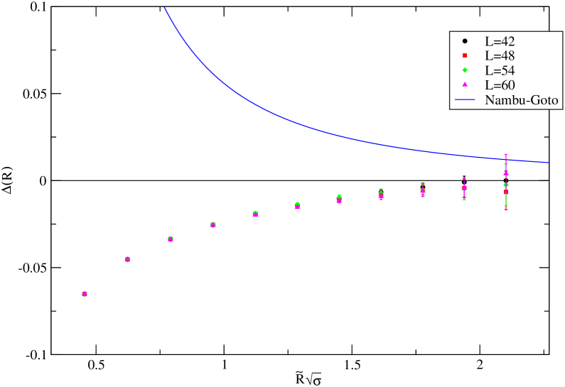
Figure 1: Deviation of the results of our numerical simulations at $L=42$, 48,54, 60 and of the Nambu-Goto string model truncated at the second order (continuous line) from the free bosonic string approximation.

Our first goal is to estimate the dependence on $R$ of the correction to the free bosonic string behaviour. To this end the simplest option would be to fit the data. However with this approach one has to face a major objection. Due to the numerical method we use, data at different distances $R$ are correlated and the crosscorrelation matrix is so flat that keeping it into account in the fits is very difficult. To circumvent these problems we decided to assume a given correction, say $b_{\alpha}/R^{\alpha}$, extract the coefficient $b_{\alpha}$ from each one of the four data at our disposal and then check the stability of the results obtained in this way. Let us see this in more detail. Let us assume that the potential is described by

$$V(R)\equiv-\frac{1}{L}G(R)=\sigma R+k+\frac{F_{1}^{q}(R,L)}{L}+\frac{b_{\alpha}}{R^{\alpha}}$$ (48)

then it is easy to see that $\Delta(R)$ should behave as

$$\Delta(R)=-b_{\alpha}\frac{\widetilde{R}^{3}}{2}\left(\frac{1}{(R+1)^{\alpha}}+\frac{1}{(R-1)^{\alpha}}-\frac{2}{R^{\alpha}}\right)$$ (49)

From this equation one can estimate the value of the coefficient $b_{\alpha}$. It is interesting to see the physical meaning of this parameter. A typical string self-interaction term is modeled by the insertion in the Lagrangian of a quartic interaction term (as in the case of the Nambu-Goto action) and leads (see for instance [3] or [11]) to a correction with $\alpha=3$. Instead a boundary term would lead to a correction with $\alpha=2$. In particular, with our choice of notations, we have $b_{2}=-\frac{\pi b}{24}$ (see eq.(16) ).

As an example of the results of our analysis we report in table 5 the values of $b_{\alpha}$ for $\alpha=2$ and 3 for the data collected at $L=42$. For the case $\alpha=3$ the estimates at the various distances $R$ turn out to agree within the errors. The results obtained using the data collected with the other values of $L$ are fully compatible with those reported in table 5. Combining together the results collected at the four different values of $L$ (they are completely uncorrelated since they have been obtained from independent simulations), we obtain as our final estimate for $b_{3}$ the value $b_{3}=0.145(15)$

$R$	$b_{2}$	$b_{3}$
8	0.038(2)	0.15(1)
9	0.032(3)	0.14(1)
10	0.022(5)	0.11(3)
11	0.014(9)	0.08(5)

Table 5: Values of $b_{2}$ and $b_{3}$ from eq.(49) using the data collected with $L=42$.

Since the parameters $b_{\alpha}$ are dimensionful quantities, it is useful to study the dimensionless ratios

$$\gamma_{\alpha}\equiv b_{\alpha}\sigma^{(\alpha-1)/2}$$ (50)

This will allow us to compare our results with other pure gauge theories, with other $SU(2)$ simulations performed at different couplings $\beta$ or with a theoretical model like the Nambu-Goto one. For instance, in the $\alpha=3$ case, we find:

$$\gamma_{3}=0.0038(4)$$ (51)

Unfortunately, the data do not allow to disentangle unambiguously a boundary term contribution from the one due to a quartic correction in the string action. However the stability of the numerical results for $b_{3}$ suggests that – similarly to the $SU(3)$ case in $(2+1)$ dimensions – there is no boundary term. Nevertheless, if we try to interpret the deviations from the free bosonic string as a boundary correction, we find that the boundary parameter $b$ must be negative and rather small, ranging from $b\sim-0.3$ for $R=8$ to $b\sim-0.1$ for $R=11$. Further investigations are needed to give more definite statements in this respect.

Instead, if we assume that the boundary term is absent and that the correction is completely due to a selfinteraction term in the effective string action, then from our analysis we obtain two important results which we present here and shall discuss in greater detail in section 6.

1] The value of $\gamma_{3}$ that we find is similar (but not equal within the errors) to the one obtained in the ${\sf Z\!\!\!Z}(2)$ gauge theory at $\beta=0.73107$: $\gamma_{3,{\sf Z\!\!\!Z}(2)}=0.0047(1)$ [21].

2] The value of $\gamma_{3}$ that we obtain is definitely different from the Nambu-Goto expectation $\gamma_{3,NG}\equiv-\frac{\pi^{2}}{1152}=-0.00857..$ (see eq.(9) ) which turns out to be opposite in sign and more or less double in magnitude. It is important to stress that a similar disagreement in the short distance regime was recently reported in [10, 13, 21].

4.1 Estimate of $\sigma$

Our short distance/low $T$ results allow an estimate for the string tension which turns out to be much more accurate than the existing ones at the considered value of $\beta$. Again, as discussed above, we cannot use a simple minded fit to obtain $\sigma$ from our data. We have chosen to use the results of the previous analysis to extract, for each value of $R$, an estimate of the string tension from the measurements of $Q(R)$. The stability of the extracted values as a function of $R$ also gives us a test of reliability. Based on the previous analysis of the corrections to the free bosonic string, we have assumed no boundary term and we have estimated $\sigma$ as

$$\sigma=Q(R)+\frac{\pi}{24}\left(\frac{1}{R+1}-\frac{1}{R}\right)-b_{3}\left(\frac{1}{(R+1)^{3}}-\frac{1}{R^{3}}\right)$$ (52)

using $b_{3}=0.145$. The results are reported in table 6. Interestingly, we note that, for each one of the four values of $L$, the data are compatible within the errors for all the values $R>R_{c}$, i.e. for $R\geq 8$. For each $L$ we consider the $R=8$ result as our best estimate for $\sigma$ since it is the one with the smallest uncertainty. The four values of $L$ are independent experiments and we can average over them yielding the final estimate $\sigma=0.025900(12)$. It is interesting to compare this result with the existing ones. In ref. [23] we find two different direct estimates obtained from two different lattice sizes: $\sigma=0.02611(19)$ for $L=24$ and $\sigma=0.02631(13)$ for $L=32$. Using the perturbative formula (40) one obtains a value inbetween, but with a much larger uncertainty $\sigma=0.02622(45)$. Our result is compatible with this last estimate, but it is definitely smaller than the two direct estimates. Finally it is also interesting to observe that the same pattern seems to be present in the results of [12] at $\beta=10$. At this value of $\beta$, eq.(40) gives $\sigma=0.02085(37)$ while ref.[12] obtains $\sigma=0.02065(6)$ which, as in our case, is smaller than the extrapolated one even if compatible within the error bars.

$R$	$L=42$	$L=48$	$L=54$	$L=60$
2	0.031400(11)	0.0313938(87)	0.0313751(10)	0.0313932(73)
3	0.026578(14)	0.026569(11)	0.026545(13)	0.0265706(96)
4	0.025993(17)	0.025983(14)	0.025955(16)	0.025987(12)
5	0.025915(20)	0.025904(16)	0.025873(19)	0.025911(14)
6	0.025911(22)	0.025898(18)	0.025865(21)	0.025909(16)
7	0.025914(25)	0.025901(20)	0.025865(24)	0.025915(17)
8	0.025914(27)	0.025902(22)	0.025863(26)	0.025920(19)
9	0.025912(29)	0.025901(23)	0.025859(29)	0.025922(22)
10	0.025907(31)	0.025899(25)	0.025855(32)	0.025922(24)
11	0.025902(34)	0.025895(28)	0.025852(35)	0.025920(28)
12	0.025896(36)	0.025893(32)	0.025851(40)	0.025918(33)
13	0.025890(40)	0.025894(38)	0.025848(48)	0.025910(40)

Table 6: Values of $\sigma$ extracted using eq.(52) and the data of table 3 as input.

4.2 Scaling behaviour of $\gamma_{3}$

In order to test the scaling behaviour of the corrections we have found at $\beta=9$, we have performed the same analysis on a data set collected at $\beta=7.5$ on a $32^{2}\times 48$ lattice. We have observed the same behaviour as at $\beta=9$ and – including in this case also the values at $R=6$ and 7 since $R_{c}=5$ – we have obtained

$$b_{3}=0.08(2)~{}~{}~{}~{}~{}\sigma=0.03856(4)$$ (53)

From these data we estimate $\gamma_{3}=0.0031(7)$. This value is compatible with the one obtained at $\beta=9$, indicating that the observed corrections are not due to scaling violations. This is well exemplified in the figure 2 where the data for $\Delta(R)$ for the two samples ($\beta=9,\,L=48$ and $\beta=7.5,\,L=48$) are compared as a function of the scaling variable $\widetilde{R}\sqrt{\sigma}$. In table 7 we report the results for $Q(R)$ and $c(R)$ we have obtained at $\beta=7.5$.

$R$	$Q(R)$	$c(R)$
2	0.054827(13)	—
3	0.047808(17)	0.077682(44)
4	0.044476(20)	0.094185(99)
5	0.042658(22)	0.10532(19)
6	0.041559(25)	0.11301(33)
7	0.040845(27)	0.11832(56)
8	0.040357(30)	0.12201(94)
9	0.040008(32)	0.1247(16)
10	0.039746(36)	0.1288(28)
11	0.039550(41)	0.1288(54)
12	0.039404(49)	0.125(11)
13	0.039304(66)	0.109(28)

Table 7: Values of $Q(R)$ and $c(R)$ for the simulation at $\beta=7.5$ on a $32^{2}\times 48$ lattice.

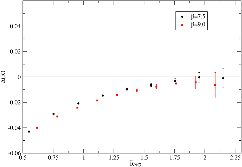
Figure 2: Comparison of the results for $\Delta(R)$ as a function of the scaling variable $\widetilde{R}\sqrt{\sigma}$ for the two samples: $\beta=9,~{}L=48$ and $\beta=7.5,~{}L=48$

5 Analysis of the long distance/high $T$ data

In this section we discuss the results we have obtained in the long distance/high $T$ regime. Our numerical simulations have been performed on a lattice with temporal extent $L=8$. The values we have obtained for $Q(R)$ and $c(R)$ are reported in table 8.

$R$	$Q(R)$	$c(R)$
2	0.037412(41)	—
3	0.030931(49)	0.071497(73)
4	0.027558(57)	0.09488(18)
5	0.025497(65)	0.11847(35)
6	0.024094(72)	0.14288(60)
7	0.023066(80)	0.16832(94)
8	0.022274(87)	0.1948(14)
9	0.021643(94)	0.2222(20)
10	0.02113(10)	0.2505(27)
11	0.02069(11)	0.2792(36)
12	0.02032(11)	0.3080(47)
13	0.02000(12)	0.3380(61)
14	0.01973(13)	0.3683(76)
15	0.01948(14)	0.3981(94)
16	0.01926(15)	0.430(11)
17	0.01905(15)	0.459(14)
18	0.01887(16)	0.491(17)
19	0.01869(17)	0.526(20)

Table 8: Values of $Q(R)$ and $c(R)$ for $L=8$ at $\beta=9$.

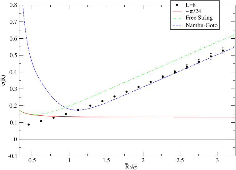
Figure 3: Comparison of the numerical results for $c(R)$ at $L=8$, $\beta=9$, with the expectations for the free bosonic string (dashed-dotted line) and with the Nambu-Goto string model truncated at the second order (dashed line). The continuous line is what one would find assuming a correction to the linear behaviour like the Lüscher term $\pi/24R$.

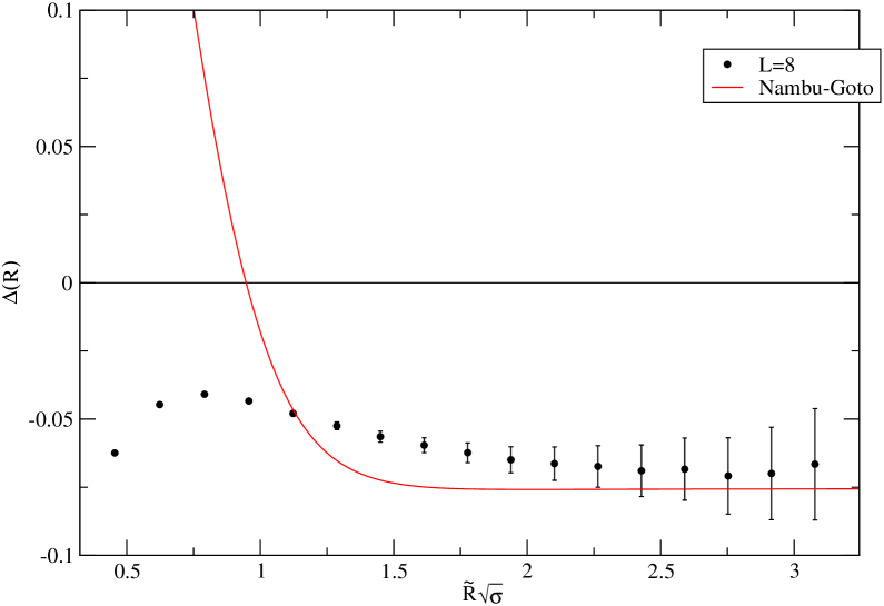
Figure 4: Deviation of the results of our numerical simulation at $L=8$ and of the Nambu-Goto string model truncated at the second order (continuous line) from the free bosonic string approximation.

Figure 5: Comparison of the numerical results for $(Q(R)-\sigma)$ at $L=8$, $\beta=9$, with the expectations for the free bosonic string (continuous line) and for the Nambu-Goto string truncated at the second order (dashed line).

These data show that in the short distance/high $T$ regime the behaviour of $c(R)$ is completely different from the one observed in the long distance/low $T$ case. There is no evidence of a convergence toward the coefficient of the Lüscher term in 3 dimensions, $\pi/24$, but instead a linearly rising behaviour is observed (see figure 3). The reason is that most of the data are in the $2R>L$ regime where a linearly rising behaviour for $c(R)$ is exactly what one expects from the free bosonic effective string model eq. (37). Let us stress that this agreement is highly non trivial and represents a very important test of the effective string description for the static quark potential. As a matter of fact, since eq. (37) is obtained by modular transforming the Dedekind function, its agreement with the numerical data is actually a test of the whole functional form of the effective string correction. In other words the agreement is obtained only keeping into account all the exponentially decreasing terms contained in the Dedekind function (which are mandatory ingredients in the modular transformation). Thus, even if in a rather indirect way, it could be considered as a test of the fact that the spectrum of the model in the short distance/low $T$ regime should be the one predicted by the bosonic effective string model. This seems to disagree with the results recently discussed in [13], where the authors investigate the spectrum of the stable excitations of the confining flux tube. From this study it turns out that below 1$fm$ – i.e. for a range of distances where the Lüscher term is already observed in the ground state of the static quark potential – the spectrum of the flux tube excitations is instead grossly distorted w.r.t. the expectations based on the effective string description. Further studies are needed to better understand the connection between our indirect test and the direct numerical evidence of [13].

Following the above comment, it is also important to notice that in the long distance/high $T$ regime any attempt to fit the data with a “Lüscher”-type correction $c(R)\sim\pi/24$ leads to a complete disagreement with the numerical simulations (see the continuous line in figure 3) already for values of $R$ comparable with the inverse temperature. This is a rather important remark, since this fitting procedure is very common in the literature and, in this regime, could lead to an apparent and erroneous rejection of the effective string model or to a systematic error in the estimate of $\sigma$.

The difference between the free bosonic string and the Nambu-Goto model is, in general, very small, but it increases as the temperature increases. The choice of $L=8$ was motivated exactly by this consideration since at this temperature the difference between the two effective string predictions is definitively larger than the errors of our simulation and we can discriminate between them. As figure 4 shows, the situation in the long distance/high $T$ regime is completely different from the short distance/low $T$ one discussed in the previous section. In fact $\Delta(R)$ has now the same sign of the Nambu-Goto prediction and its shape and numerical value are in good agreement with it. This is one of our main results and suggests that, contrary to what happens in the short distance/low $T$ regime, the Nambu-Goto string can give a reliable description for the static quark potential in the large distance/high $T$ regime. Interestingly, a similar scenario also occurs in the 3-d ${\sf Z\!\!\!Z}(2)$ gauge theory [11].

In principle one could interpret the deviation from the free bosonic string behaviour in figure 4 as due to a boundary term instead of a Nambu-Goto like correction. This requires $b$ to have a value $b\sim-0.8$ which agrees in sign with the one that we find under the same assumptions in the short distance/low $T$ regime, but it is from three to eight times bigger. Again, this could suggest that the deviations in $\Delta(R)$ might not be due to a boundary term. As a matter of fact the value of $b$ could be fixed without ambiguities looking at different values of $L$ since the boundary correction and the Nambu-Goto one have a different $L$ dependence. However this is not easy since it would require to keep the high precision of our results also for larger values of $L$. This type of analysis was indeed performed in the case of the 3-d ${\sf Z\!\!\!Z}(2)$ gauge theory [21] where, thanks to the different nature of the simulation algorithm [27, 28, 11], this level of precision can be reached for arbitrary values of $L$ and $R$. We plan to address this type of analysis for the $SU(2)$ model in a forthcoming publication.

Further interesting informations can be obtained from $Q(R)$ (see figure 5). As we mentioned in section 1, the behaviour of $Q(R)$ is dominated by $\sigma$. However in the present case we can use the very precise value for sigma obtained in section 4. In figure 5 we plot the difference $(Q(R)-\sigma)$ as a function of $R$. Thanks to the accurate estimate of $\sigma$, the systematic uncertainty in this difference due to $\sigma$ turns out to be negligible w.r.t. the statistical errors of $Q(R)$. Figure 5 shows that the numerical estimates lie below the Nambu-Goto prediction truncated at the second order. On one hand, this means that the Nambu-Goto prediction truncated at the second order describes the data better than the free bosonic string, on the other hand it also suggests that the higher order terms in the expansion of the Nambu-Goto action could fill the remaining gap between numerical data and theoretical estimates. Finally let us notice that a similar agreement with the Nambu-Goto model was also recently observed in the large distance/high $T$ data for the 3-d ${\sf Z\!\!\!Z}(2)$ gauge theory.

6 Comparison with ${\sf Z\!\!\!Z}(2)$ and $SU(3)$ gauge theories

It is very interesting to compare our short distance/low $T$ results with those recently obtained for the ${\sf Z\!\!\!Z}(2)$ [8, 11, 21] and $SU(3)$ [9] gauge theories. Among the $SU(3)$ data published in [9] we have selected, for our comparison, the sample at $\beta=20$ (see the data in table 3 of ref. [9]) which is the one with the larger set of data. For the ${\sf Z\!\!\!Z}(2)$ gauge theory we have chosen the sample at $\beta=0.73107$ and $L=80$ of ref.[21] which corresponds to a very low temperature $T/T_{c}=1/20$ and to a similar value for the lattice spacing. For the $SU(2)$ case we have used for the comparison only the $L=42$ sample which is the most precise one. The other three samples would add no further information since they are compatible within the errors. For distances $R$ large enough, the three theories show the same asymptotic behaviour. Our aim is to study the higher order corrections which characterize the approach to the asymptotic free bosonic string limit.

We plot the three data sets in figure 6. Since the three sets correspond to different values of $\sigma$, we have rescaled $R$ in units of $\sqrt{\sigma}$ in order to make a meaningful comparison.

Let us briefly comment on figure 6.

• As discussed in [9], the $SU(3)$ data are rather well described by the free string correction only and $\Delta(R)$ turns out to be very small for $R>R_{c}$.

• On the contrary, both the $SU(2)$ and the ${\sf Z\!\!\!Z}(2)$ data show rather strong deviations from the free string behaviour. These deviations are stronger in the ${\sf Z\!\!\!Z}(2)$ case than in the $SU(2)$ one.

• For all the three models the observed corrections definitely disagree with the Nambu-Goto prediction (which is not reported in the figure but it can be seen in figure 1) which has the opposite sign and is larger in magnitude.

Our conclusion is that, in 3 dimensions, the terms subleading to the free bosonic string behaviour in ${\sf Z\!\!\!Z}(2)$, $SU(2)$ and $SU(3)$ gauge theories do not show any evidence of common features. This confirms the expectation that these subleading corrections depend on the string dynamics and are thus different for the different gauge groups.

A similar comparison between the 3-d $SU(2)$ and ${\sf Z\!\!\!Z}(2)$ gauge theories for the ground state energy and for the first excited string level was recently performed in [13, 14]. In that case the two models were shown to have similar behaviours after readjusting the ratio of the string tension to the glueball mass in the ${\sf Z\!\!\!Z}(2)$ gauge theory. It would be interesting to understand if this agreement is a consequence of the rescaling or if it is instead related to the fact that the two models share the same center. This is one of the reasons for which we plan to extend our analysis also to the gauge theory with gauge group $Sp(2)$ [29, 30] which has the same center as $SU(2)$ and ${\sf Z\!\!\!Z}(2)$.

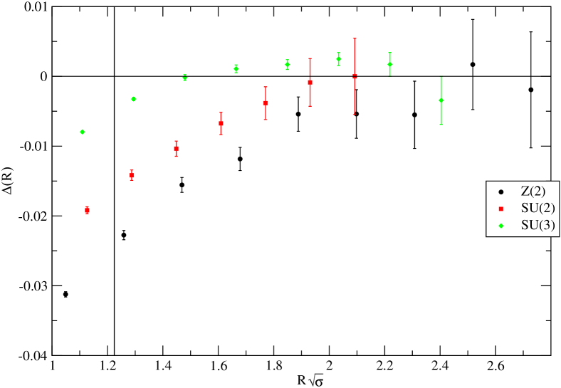
Figure 6: Values of $\Delta(R)$ in 3-d for the $SU(3)$ Yang-Mills theory (diamonds), the ${\sf Z\!\!\!Z}(2)$ gauge theory (circles) and the sample with $L=42$ of the $SU(2)$ Yang-Mills theory (squares). The vertical line corresponds to $R=R_{c}=\sqrt{1.5/\sigma}$. Here $\Delta(R)$ is evaluated considering $R$ and not $\widetilde{R}$.

7 Concluding remarks

In this paper we have studied the corrections to the linear behaviour of the static quark potential in the $SU(2)$ Yang-Mills theory in (2+1) dimensions. We have considered both the zero and the finite temperature regimes comparing the numerical results with the expectations coming from effective string descriptions of the quark interaction. Finally we have checked for common features among the effective string descriptions of ${\sf Z\!\!\!Z}(2)$, $SU(2)$ and $SU(3)$ gauge theories. Our results can be summarized as follows.

• Our numerical simulations strongly support the conjecture that the ground state of the static quark potential in the (2+1) dimensional $SU(2)$ Yang-Mills theory (as well as in all the other pure gauge theories studied up to now) is very well described by an effective string theory. Apart from subleading corrections – which can be observed at short distances and/or at high $T$ – this effective string theory is the bosonic string theory originally suggested by Lüscher, Symanzik and Weisz in [1].

• We observe deviations from the free string behaviour also in the short distance/low $T$ regime. These deviations definitely disagree with the Nambu-Goto predictions. A similar disagreement was recently observed also in the 3-d ${\sf Z\!\!\!Z}(2)$ gauge theory [10, 13, 21].

• In the large distance/high $T$ regime, we clearly observe deviations from the free bosonic string approximation. These deviations qualitatively – and, in part, also quantitatively – agree with the predictions of the Nambu-Goto action truncated at the second perturbative order.

• The large distance/high $T$ regime can be obtained by a modular transformation of the effective string results in the short distance/low $T$ regime. The observed agreement with the effective string expectation not only confirms the presence of the Lüscher term but also suggests an indirect check of the whole functional form and, in particular, of the spectrum of the excited states. However we emphasize that this is still an open question that deserves further investigations.

• Comparing the ${\sf Z\!\!\!Z}(2)$, $SU(2)$ and $SU(3)$ gauge theories, we do not find any clue for common features in the corrections to the Lüscher term among them.

In view of this last point, it would be important to understand if these analogies and differences are related to the gauge group, to its center, or are non-universal features, perhaps related to different values of the boundary term $b$. To this end it would be very interesting to extend this type of analysis to a wider set of pure gauge theories. For instance, one can consider the Yang-Mills theory with gauge group $Sp(2)$ [29, 30] which has the same center ${\sf Z\!\!\!Z}(2)$ as the group $SU(2)$ studied in this paper.

Acknowledgments. We acknowledge useful discussions with F. Gliozzi, J. Juge, J. Kuti, C. Morningstar, U.-J. Wiese. This work was partially supported by the European Commission TMR programme HPRN-CT-2002-00325 (EUCLID) as well as by the Schweizerischer Nationalfond.

References

- [1] M. Lüscher, K. Symanzik and P. Weisz, Nucl. Phys. B173 (1980) 365.
- [2] M. Lüscher, Nucl. Phys. B180 (1981) 317.
- [3] K. Dietz and T. Filk, Phys. Rev. D27 (1983) 2944.
- [4] O. Jahn and P. de Forcrand, Nucl. Phys. B (Proc. Suppl.) 129-130 (2004) 700.
- [5] M. Caselle, R. Fiore, F. Gliozzi, M. Hasenbusch and P. Provero, Nucl. Phys. B486 (1997) 245.
- [6] B. Lucini and M. Teper, Phys. Rev. D64 (2001) 105019.
- [7] S. Necco and R. Sommer, Nucl. Phys. B622 (2002) 328.
- [8] M. Caselle, M. Panero and P. Provero, JHEP 0206 (2002) 061.
- [9] M. Lüscher and P. Weisz, JHEP 0207 (2002) 049.
- [10] K. J. Juge, J. Kuti and C. Morningstar, Phys. Rev. Lett. 90 (2003) 161601.
- [11] M. Caselle, M. Hasenbusch and M. Panero, JHEP 0301 (2003) 057.
- [12] P. Majumdar, Nucl. Phys. B664 (2003) 213.
- [13] K. J. Juge, J. Kuti and C. Morningstar, Nucl. Phys. B (Proc. Suppl.) 129-130 (2004) 686.
- [14] K. J. Juge, J. Kuti and C. Morningstar, hep-lat/0401032.
- [15] K. J. Juge, J. Kuti and C. Morningstar, hep-lat/0312019.
- [16] M. Caselle, M. Pepe and A. Rago, Nucl. Phys. B (Proc. Suppl.) 129-130 (2004) 721.
- [17] Y. Koma, M. Koma and P. Majumdar, hep-lat/0311016.
- [18] M. Lüscher and P. Weisz, JHEP 0109 (2001) 010.
- [19] M. Caselle, M. Hasenbusch and M. Panero, Nucl. Phys. B (Proc. Suppl.) 129-130 (2004) 593.
- [20] M. Caselle, M. Hasenbusch and M. Panero, hep-lat/0403004, to be published in JHEP.
- [21] M. Caselle, M. Panero and M. Hasenbusch, hep-lat/0312005.
- [22] R. Sommer, Nucl. Phys. B411 (1994) 839.
- [23] M. J. Teper, Phys. Rev. D59 014512 (1999).
- [24] B. Svetitsky and L. G. Yaffe, Nucl. Phys. B210 (1982) 423.
- [25] G. Parisi, R. Petronzio and F. Rapuano, Phys. Lett. B128 (1983) 418.
- [26] H. B. Meyer, JHEP 0401 (2004) 030.
- [27] P. de Forcrand, M. D’Elia and M. Pepe, Phys. Rev. Lett. 86 (2001) 1438.
- [28] M. Pepe and P. De Forcrand, Nucl. Phys. B (Proc. Suppl.) 106 (2002) 914.
- [29] K. Holland, M. Pepe and U. J. Wiese, Nucl. Phys. B (Proc. Suppl.) 129-130 (2004) 712.
- [30] K. Holland, M. Pepe and U. J. Wiese, hep-lat/0312022, to be published in Nucl. Phys. B.