Abstract

The Yang-Mills theory lies at the heart of our understanding of elementary particle interactions. For the strong nuclear forces, we must understand this theory in the strong coupling regime. The primary technique for this is the lattice. While basically an ultraviolet regulator, the lattice avoids the use of a perturbative expansion. I discuss some of the historical circumstances that drove us to this approach, which has had immense success, convincingly demonstrating quark confinement and obtaining crucial properties of the strong interactions from first principles.

Chapter 0 YANG-MILLS FIELDS AND THE LATTICE

1 Introduction

Originally motivated to extend the gauge theory of quantum electrodynamics to include isospin, the Yang-Mills theory has become a core ingredient of all modern theories of elementary particles. With the particular application to the strong interactions of quarks interacting by exchanging non-Abelian gauge gluons, some rather unique issues arise. In particular, asymptotic freedom and dimensional transmutation imply that low energy physics is controlled by large effective coupling constants. Long distance phenomena, such as chiral symmetry breaking and quark confinement, lie outside the realm of accessibility to the traditional Feynman diagram approach. This drove us to new approaches, amongst which the lattice has proven the most successful.

This chapter is a personal reminiscence of how the lattice approach was developed and grew to become the dominant approach to study non-perturbative effects in quantum field theory. Along the way we will see that the contributions have been both practical and fundamental. They are practical in the sense that we can perform quantitative computer calculations of non-perturbative effects in the strong interactions. They are fundamental in the sense that the lattice gives deep insights into the workings of relativistic field theory, in particular into anomalous features that distinguish between the classical and the quantum theories.

2 Before the lattice

I begin by summarizing the situation in particle physics in the late 60’s, when I was a graduate student. Quantum-electrodynamics had already been immensely successful, but that theory was in some sense “done.” While hard calculations remained, and indeed still remain, there was no major conceptual advance remaining.

These were the years when the “eightfold way” for describing multiplets of particles had recently gained widespread acceptance. The idea of “quarks” was around, but with considerable caution about assigning them any physical reality; maybe they were nothing but a useful mathematical construct. A few insightful theorists were working on the weak interactions, and the basic electroweak unification was beginning to emerge. The SLAC experiments were observing substantial inelastic electron-proton scattering at large angles, and this was quickly interpreted as evidence for substructure, with the term “parton” coming into play. While occasionally there were speculations relating quarks and partons, people tended to be rather cautious about pushing this too hard.

A crucial feature of the time was that the extension of quantum electrodynamics to a meson-nucleon field theory was failing miserably. The analog of the electromagnetic coupling had a value about 15, in comparison with the 1/137 of QED. This meant that higher order corrections to perturbative processes were substantially larger than the initial calculations. There was no known small parameter in which to expand.

In frustration over this situation, much of the particle theory community set aside traditional quantum field theoretical methods and explored the possibility that particle interactions might be completely determined by fundamental postulates such as analyticity and unitarity. This “S-matrix” approach raised the deep question of just “what is elementary?” A delta baryon might be regarded as a combination of a proton and a pion, but it would be just as correct to regard the proton as a bound state of a pion with a delta. All particles are bound together by exchanging themselves. These “dual” views of the basic objects of the theory persist today in string theory.

3 The birth of QCD

As we entered the 1970’s, partons were increasingly identified with quarks. This shift was pushed by two dramatic theoretical accomplishments. First was the proof of renormalizability for non-Abelian gauge theories[1], giving confidence that these elegant mathematical structures[2] might have something to do with reality. Second was the discovery of asymptotic freedom, the fact that interactions in Yang-Mills theories become weaker at short distances[3]. Indeed, this was quickly connected with the point-like structures hinted at in the SLAC experiments. Out of these ideas evolved QCD, the theory of quark confining dynamics.

The viability of this picture depended upon the concept of “confinement.” While there was strong evidence for quark substructure, no free quarks were ever observed. This was particularly puzzling given the nearly free nature of their apparent interactions inside the nucleon. This returns us to the question of “what is elementary?” Are the fundamental objects the physical particles we see in the laboratory or are they these postulated quarks and gluons?

Struggling with this paradox led to the now standard flux-tube picture of confinement. The eight gluons are analogues of photons except that they carry “charge” with respect to each other. Without confinement gluons would presumably be free massless particles like the photon. But a massless charged particle would be a rather peculiar object. Indeed, what happens to the self energy in the electric fields around a gluon? Such questions naturally lead to a conjectured instability of the æther that removes zero mass gluons from the spectrum. This is to be done in a way that does not violate Gauss’s law. Note that a Coulombic $1/r^{2}$ field is a solution of the equations of a massless field, not a massive one. Without massless particles in the spectrum, such a spreading of the gluonic flux is not allowed since it cannot satisfy the appropriate equations in the weak field limit. But from Gauss’s law, the field lines emanating from a quark cannot end. Instead of spreading in the inverse square manner, the flux lines cluster together, forming a tube emanating from the quark and ultimately ending on an anti-quark as sketched in Fig. 1. This structure is a real physical object, and grows in length as the quark and anti-quark are pulled apart. The resulting force is constant at long distance, and is measured via the spectrum of high angular momentum states, organized into the famous “Regge trajectories.” In physical units, the flux tube pulls with a strength of about 14 tons.

The reason a quark cannot be isolated is similar to the reason that a piece of string cannot have just one end. Of course one can’t have a piece of string with three ends either, but this is the reason for the underlying $SU(3)$ group theory, wherein three fundamental charges can form a neutral singlet. It is important to emphasize that the confinement phenomenon cannot be seen in perturbation theory; when the coupling is turned off, the spectrum becomes free quarks and gluons, dramatically different than the pions and protons of the interacting theory.

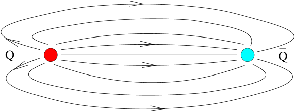
Figure 1: A tube of gluonic flux connects quarks and anti-quarks. The strength of this string is 14 tons.

4 The 70’s revolution

The discoveries related to the Yang-Mills theory were just the beginning of a revolutionary sequence of events in particle physics. Perhaps the most dramatic was the discovery of the $J/\psi$ particle[4]. The interpretation of this object and its partners as bound states of heavy quarks provided the hydrogen atom of QCD. The idea of quarks became inescapable; field theory was reborn. The $SU(3)$ non-Abelian gauge theory of the strong interactions was combined with the recently developed electroweak theory to become the durable “standard model.”

This same period also witnessed several additional remarkable events on the more theoretical front. Non-linear effects in classical field theories were shown to have deep consequences for their quantum counterparts. Classical “lumps” represented a new way to get particles out of a quantum field theory[5]. Much of the progress here was in two dimensions, where techniques such as “bosonization” showed equivalences between theories of drastically different appearance. A boson in one approach might appear as a bound state of fermions in another, but in terms of the respective Lagrangian approaches, they were equally fundamental. Again, we were faced with the question “what is elementary?” Of course modern string theory is discovering multitudes of “dualities” that continue to raise this same question.

The ensuing obsession with classical solutions quickly led to the discovery [6] of “pseudo-particles” or “instantons” as classical solutions of the four dimensional Yang-Mills theory in Euclidean space time. See R. Jackiw’s contribution to this volume. These turned out to be intimately related to the famous anomalies in current algebra, and gave a simple mechanism to generate the anomalous masses of such particles as the $\eta^{\prime}$. These effects were all inherently non-perturbative, having an explicit exponential dependence in the inverse coupling. If the coupling is reduced in the theory with a fixed cutoff, these effects fall to zero faster than any power of the coupling.

This slew of discoveries had deep implications: field theory can display much more structure than seen from the traditional analysis of Feynman diagrams. But this in turn had crucial consequences for practical calculations. Field theory is notorious for divergences requiring regularization. The bare mass and charge are divergent quantities. They are not the physical observables, which must be defined in terms of physical processes. To calculate, a “regulator” is required to tame the divergences, and when physical quantities are related to each other, any regulator dependence should drop out.

The need for controlling infinities had, of course, been known since the early days of QED. But all regulators in common use were based on Feynman diagrams; the theorist would calculate diagrams until one diverged, and that diagram was then cut off. Numerous schemes were devised for this purpose, ranging from the Pauli-Villars approach to forest formulae to dimensional regularization. But with the increasing realization that non-perturbative phenomena were crucial, it was becoming clear that we needed a “non-perturbative” regulator, independent of diagrams.

5 The lattice

The necessary tool appeared with Wilson’s lattice theory. He originally presented this as an example of a model exhibiting confinement. The strong coupling expansion has a non-zero radius of convergence, allowing a rigorous demonstration of confinement, albeit in an unphysical limit. The resulting spectrum has exactly the desired properties; only gauge singlet bound states of quarks and gluons can propagate.

This was not the first time that the basic structure of lattice gauge theory had been written down. A few years earlier, Wegner[7] presented a $Z_{2}$ lattice gauge model as an example of a system possessing a phase transition but not exhibiting any local order parameter. In his thesis, Jan Smit[8] described using a lattice regulator to formulate gauge theories outside of perturbation theory. The time was clearly ripe for the development of such a regulator. Very quickly after Wilson’s suggestion, Balian, Drouffe, and Itzykson[9] explored an amazingly wide variety of aspects of these models.

To reiterate, the primary role of the lattice is to provide a non-perturbative cutoff. Space is not really meant to be a crystal, the lattice is a mathematical trick. It provides a minimum wavelength through the lattice spacing $a$, i.e. a maximum momentum of $\pi/a$. Path summations become well defined ordinary integrals. By avoiding the convergence difficulties of perturbation theory, the lattice provides a route towards the rigorous definition of quantum field theory.

The approach, however, had a marvelous side effect. By discreetly making the system discrete, it becomes sufficiently well defined to be placed on a computer. This was fairly straightforward, and came at the same time that computers were growing rapidly in power. Indeed, numerical simulations and computer capabilities have continued to grow together, making these efforts the mainstay of modern lattice gauge theory.

6 Gauge fields and phases

As formulated by Wilson, the lattice cutoff is quite remarkable in that it manages to keep exact many of the concepts of a gauge theory. Of course, there are many ways to think of a gauge theory, and this is apparent in the variety of viewpoints expressed in the contributions to this volume.

At the most simplistic level, a Yang-Mills theory is just electrodynamics embellished with isospin symmetry. By working directly with elements of the gauge group, this is inherent in lattice gauge theory from the start.

At another level, a gauge theory is a theory of phases acquired by a particle as it passes through space time. Using group elements on links directly gives this connection, with the phase associated with some world-line being the product of these elements along the path in question. Of course, for the Yang-Mills theory the concept of “phase” becomes a rotation in the internal symmetry group.

A gauge theory is a theory with a local symmetry. With the Wilson action being formulated in terms of products of group elements around closed loops, this symmetry remains exact even with the cutoff in place.

In perturbative discussions, the local symmetry forces a gauge fixing to remove a formal infinity of different gauges. For the lattice formulation, however, the use of a compact representation for the group elements means that the integration over all gauges is finite. To study gauge invariant observables, no gauge fixing is required to define the theory. Of course gauge fixing can still be done, and must be introduced to study more conventional gauge variant quantities such as gluon or quark propagators.

The only definition of a gauge theory that the lattice does not keep exact is how a gauge field transforms under Lorentz transformations. In a continuum theory the basic vector potential can change under a gauge transformation when transforming between frames. The lattice, of course, breaks Lorentz invariance, and thus this concept looses meaning.

7 The Wilson action

The concept of gauge fields as path dependent phases leads directly to the conventional method for formulating the quark and gluon fields on a lattice. We approximate a general quark world-line by a set of hoppings lying along lattice bonds, as sketched in Fig. 2. We then introduce the gauge field as group valued matrices on these bonds. Thus the gauge fields form a set of $SU(3)$ matrices, one such associated with every nearest neighbor bond on our four-dimensional hyper-cubic lattice.

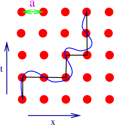
Figure 2: In lattice gauge theory the world-line describing the motion of a quark through space-time is approximated by a sequence of discrete hops. On each of these hops the quark wave function picks up a “phase” described by the gauge fields. For the strong interactions, this phase is a unitary matrix in the group $SU(3)$.

In terms of these matrices, the gauge field dynamics takes a simple natural form. In analogy with regarding electromagnetic flux as the generalized curl of the vector potential, we are led to identify the flux through an elementary square, or “plaquette,” on the lattice with the phase factor obtained on running around that plaquette; see Fig. 3. Spatial plaquettes represent the “magnetic” effects and plaquettes with one direction time-like give the “electric” fields. This motivates the conventional “action” used for the gauge fields as a sum over all the elementary squares of the lattice. Around each square we multiply the phases and to get a real number we take the real part of the trace

$$S_{g}=\sum_{p}{\rm Re\ Tr}\prod_{l\in p}U_{l}$$ (1)

Here the fundamental squares are denoted $p$ and the links $l$. As we are dealing with non-commuting matrices, the product around the square is meant to be ordered.

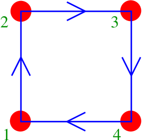
Figure 3: In analogy with Stoke’s law, the flux through an elementary square of the lattice is found from the product of gauge matrices around that square. The dynamics is determined by adding the real part of the trace of this product over all elementary squares. This “action” is inserted into a “path integral.” The resulting construction is formally a partition function for a system of “spins” existing in the group $SU(3)$.

To formulate the quantum theory of this system one usually uses the Feynman path integral. For this, exponentiate the action and integrate over all dynamical variables to construct

$$Z=\int(dU)e^{-\beta S}$$ (2)

where the parameter $\beta$ controls the bare coupling. This converts the three space dimensional quantum field theory of gluons into a classical statistical mechanical system in four space-time dimensions. Such a many-degree-of-freedom statistical system cries out for Monte Carlo simulation, which now dominates the field of lattice QCD. Note the close analogy with a magnetic system; we could think of our matrices as “spins” interacting through a four spin coupling expressed in terms of the plaquettes.

The formulation is in Euclidean four dimensional space, based on an underlying replacement of the time evolution operator $e^{-iHt}$ by $e^{-Ht}$. Despite involving the same Hamiltonian, excited states are inherently suppressed and information on high energy scattering is particularly hard to extract. However low energy states and matrix elements are the natural physical quantities to explore numerically. This is the bread and butter of the lattice theorist. Indeed, the simulations reproduce the qualitative spectrum of stable hadrons quite well. Matrix elements currently under intense study are playing a crucial role in ongoing tests of the standard model of particle physics.

8 A paucity of parameters

Now I wish to reiterate one of the most remarkable aspects of the theory of quarks and gluons, the small number of adjustable parameters. To begin with, the lattice spacing itself is not an observable. We are using the lattice to define the theory, and thus for physics we are interested in the continuum limit $a\rightarrow 0$. Then there is the coupling constant, which is also not a physical parameter due to the phenomenon of asymptotic freedom. The lattice works directly with a bare coupling, and in the continuum limit this should vanish as predicted by asymptotic freedom

$$g_{0}^{2}\sim{1\over\log(1/\Lambda a)}\rightarrow 0$$ (3)

In the process, the coupling is replaced by an overall scale $\Lambda$, which might be regarded as an integration constant for the renormalization group equation. Coleman and Weinberg[10] gave this phenomenon the marvelous name “dimensional transmutation.” Of course an overall scale is not really something we should expect to calculate from first principles. Its value would depend on the units chosen, be they furlongs or light-fortnights.

Next consider the quark masses. These also renormalize to zero as a power of the coupling in the continuum limit. Removing this divergence, we can define a renormalized quark mass, which is a second integration constant of the renormalization group equations. One such constant $M_{i}$ is needed for each quark “flavor” or species $i$. Up to an irrelevant overall scale, the physical theory is then a function only of the dimensionless ratios $M_{i}/\Lambda$. These are the only free parameters in the strong interactions. The origin of the underlying masses remains one of the outstanding mysteries of particle physics.

With multiple flavors, the massless quark limit gives a rather remarkable theory, one with no undetermined dimensionless parameters. This limit is not terribly far from reality; chiral symmetry breaking should give massless pions, and experimentally the pion is considerably lighter than the next non-strange hadron, the rho. A theory of two massless quarks is a fair approximation to the strong interactions at intermediate energies. In this limit all dimensionless ratios should be calculable from first principles, including quantities such as the rho to nucleon mass ratio. The one flavor theory provides an interesting intellectual exercise; indeed, the massless one flavor theory is not uniquely defined[11].

Since it is absorbed into an overall scale, the strong coupling constant at any physical scale is not an input parameter, but should be determined from first principles. Such a calculation has gotten lattice gauge theory into the famous particle data group tables[12]. With appropriate definition a recent lattice result is

$$\alpha_{s}(M_{Z})=0.115\pm 0.003$$ (4)

where the input is details of the charmonium spectrum.

9 Numerical simulation

While other techniques exist, such as strong coupling expansions, large scale numerical simulations currently dominate lattice gauge theory. They are based on attempts to evaluate the path integral

$$Z=\int(dU)\ e^{-\beta S}$$ (5)

with $\beta$ proportional to the inverse bare coupling squared. A direct evaluation of such an integral has pitfalls. At first sight, the basic size of the calculation is overwhelming. Considering a $10^{4}$ lattice, small by today standards, there are 40,000 links. For each is an $SU(3)$ matrix, parametrized by 8 numbers. Thus we have a $10^{4}\times 4\times 8=320,000$ dimensional integral. One might try to replace this with a discrete sum over values of the integrand. If we make the extreme approximation of using only two points per dimension, this gives a sum with

$$2^{320,000}=3.8\times 10^{96,329}$$ (6)

terms! Of course, computers are getting pretty fast, but one should remember that the age of universe is only $\sim 10^{27}$ nanoseconds.

These huge numbers suggest a statistical treatment. Indeed, the above integral is formally just a partition function. Consider a more familiar statistical system, such as a glass of beer. There are a huge number of ways of arranging the atoms of carbon, hydrogen, oxygen, etc. that still leaves us with a glass of beer. We don’t need to know all those arrangements, we only need a dozen or so “typical” glasses to know all the important properties.

This is the basis of the Monte Carlo approach. The analogy with a partition function and the role of ${1\over\beta}$ as a temperature enables the use of standard techniques to obtain “typical” equilibrium configurations, where the probability of any given configuration is given by the Boltzmann weight

$$P(C)\sim e^{-\beta S(C)}$$ (7)

For this we use a Markov process, making changes in the current configuration

$$C\rightarrow C^{\prime}\rightarrow\ldots$$ (8)

biased by the desired weight.

The idea is easily demonstrated with the example of $Z_{2}$ lattice gauge theory[13]. For this toy model the links are allowed to take only two values, either plus or minus unity. One sets up a loop over the lattice variables. When looking at a particular link, calculate the probability for it to have value $1$

$$P(1)={e^{-\beta S(1)}\over e^{-\beta S(1)}+e^{-\beta S(-1)}}$$ (9)

Then pull out a roulette wheel and select either 1 or $-1$ biased by this weight. Lattice gauge Monte-Carlo programs are by nature quite simple. They are basically a set of nested loops surrounding a random change of the fundamental variables.

Extending this to fields in larger manifolds, such as the $SU(3)$ matrices representing the gluon fields, is straightforward. The algorithms are usually based on a detailed balance condition for a local change of fields taking configuration $C$ to configuration $C^{\prime}$. If probabilities for making these changes in one step satisfy

$${P(C\rightarrow C^{\prime})\over P(C^{\prime}\rightarrow C)}={e^{-\beta S(C^{\prime})}\over e^{-\beta S(C)}}$$ (10)

it is straightforward to prove that any ensemble of configurations approaches the equilibrium ensemble.

The results of these simulations have been fantastic, giving first principles calculations of interacting quantum field theory. I will just mention two examples. The early result that bolstered the lattice into mainstream particle physics was the convincing demonstration of the confinement phenomenon. The force between two quark sources indeed remains constant at large distances.

Another accomplishment for which the lattice excels over all other methods has been the study the deconfinement of quarks and gluons into a plasma at a temperature of about 170–190 Mev[14]. Indeed, the lattice is a unique quantitative tool capable of making precise predictions for this temperature. The method is based on the fact that the Euclidean path integral in a finite temporal box directly gives the physical finite temperature partition function, where the size of the box is proportional to the inverse temperature. This transition represents the confining flux tubes becoming lost in a background plasma of virtual flux lines.

10 Quarks and random numbers

While the gauge sector of the lattice theory is in good shape, from the earliest days fermionic fields have caused annoying difficulties. Actually there are several apparently unrelated fermion problems. The first is an algorithmic one. The quark operators are not ordinary numbers, but anti-commuting operators in a Grassmann space. As such, the exponentiated action itself is an operator. This makes comparison with random numbers problematic.

Until relatively recently, most lattice work with quarks was done in the so called “valence” or “quenched” approximation. A pure gauge simulation provides a set of background gauge fields in which the propagation of quarks is calculated. The approximation is to ignore any feedback of the quarks on the gauge fields. As the quarks involve large sparse matrices, the conjugate gradient algorithm is ideally suited. Combining the resulting propagators into hadronic combinations gives predictions on physical quantities such as spectra, matrix elements, etc. The rather random nature of the relevant background fields has hampered application of standard multi-scale techniques, but more work in this area is needed. The main issue with the valence approximation is that systematic errors are not under precise control.

Over the years various clever tricks for dealing with dynamical quarks have been developed; numerous ongoing large scale Monte Carlo simulations do involve dynamical fermions. The algorithms used are all essentially based on an initial analytic integration of the quarks to give a determinant. This, however, is the determinant of a rather large matrix, the size being the number of lattice sites times the number of fermion field components, with the latter including spinor, flavor, and color factors. For a Monte Carlo evolution we need to know how this determinant changes with random changes in the gauge field. Introducing auxiliary bosonic fields reduces the problem to doing large sparse matrix inversions inside the Monte Carlo loop. It is these inversions that currently dominate the required compute time. In my opinion, the algorithms working directly with these large matrices remain quite awkward. I often wonder if there is some more direct way to treat fermions without the initial analytic integration. On small systems direct evaluation of Grassmann integrals by machine is possible[16, 17], although the approach appears to be inherently exponential in the system volume.

The algorithmic problem becomes considerably more serious when a chemical potential generating a background baryon density is present. In this case the required determinant is not positive; it cannot be incorporated as a weight in a Monte Carlo procedure. This is particularly frustrating in the light of striking predictions of super-conducting phases at large chemical potential[18]. This is perhaps the most serious unsolved problem in lattice gauge theory today.

11 Chirality, anomalies, and the lattice

While the difficulty in simulating Grassmann dynamics is a major issue, further conceptual fermion problems concern chiral issues. These are intimately entwined with the anomalous differences between classical and quantum field theories. Indeed, while the lattice is usually just thought of as a numerical technique, it also provides a path to understanding many subtleties of quantum field theory. As a full non-perturbative regulator, the lattice provides a foundation for defining quantum field theory.

It is well known that some classical symmetries do not survive quantization. The most basic example, the scale anomaly, has been so fully absorbed into the lattice lore that it is rarely mentioned. The classical Yang-Mills theory is scale invariant and depends in a non-trivial way on the coupling constant. The quantum theory, however, is not at all scale invariant. Indeed, it is a theory of massive glueballs and the masses these particles set a definite scale.

When the quark masses vanish, the classical Lagrangian for the strong interactions still contains no dimensional parameters. But the quantum theory is supposed to describe baryons and mesons, and the lightest baryon, the proton, definitely has mass. As discussed in the earlier section on parameters, this is understood through the phenomenon of “dimensional transmutation,” wherein the classical coupling constant of the theory is traded, through the process of renormalization, for an overall scale parameter[10].

The scale anomaly is perhaps the deepest, but it is not the only symmetry of the strong interactions of massless quarks that is lost upon quantization. The most famous are the anomalies in the axial-vector fermion currents[19, 20, 21], also discussed in the contributions by S. Adler and R. Jackiw to this volume. Working in a helicity basis, the classical Lagrangian has no terms to change the number of left or right handed fermions. On quantization, however, these numbers cease to be separately conserved. Technically this comes about because of the famous triangle diagram. This introduces a divergence which requires regularization via a dimensionful cutoff. For the strong interactions with its vector-like gluon couplings, this regulation is implemented so that the vector current, representing total fermion number, is conserved. But if this choice is taken, then the axial current, representing the difference of right and left handed fermion numbers, cannot be. There is a freedom in choosing which currents are conserved; however, in a gauge theory, consistency requires that gauge fields couple only to conserved currents.

In the full standard model, anomalies require some time honored conservation laws to be violated. The most famous example is baryon number, which in the standard model is sacrificed so that the chiral currents that couple to the vector bosons are conserved[22, 23]. Baryon violating semi-classical processes have been identified and must be present, although at a very low rate. While not of observable strength, at a conceptual level any scheme for non-perturbatively regulating the standard model must either contain baryon violating terms[24] or extend the model to cancel these anomalies with, say, mirror species[25, 26].

Consistency under anomalies has non-trivial implications for the allowed species of fermions. To conserve all the gauged currents of the standard model requires the cancellation of all potential anomalies in currents coupled to gauge fields. In particular, the standard model is not consistent if either the leptons or the quarks are left out. This connection between quarks and leptons is a deep subtlety of the theory and must play a key role in placing the theory on a lattice. Although these effects are extremely tiny due to the smallness of the weak coupling constant, without a precise non-perturbative regulator that is capapable of including these phenomena, it is not clear that the weak interactions fit into a meaningful field theory.

At a more phenomenological level, there are a variety of reasons that chiral symmetries are important to particle physics. Premier among these is the light nature of the pion, which is traditionally related to the spontaneous breaking of a chiral symmetry expected to become exact as the quark masses go to zero. This is the explanation as to why the pion is so much lighter than the rho meson, even though they are made of the same quarks, albeit in different spin states.

Theories unifying the various interactions also often make heavy use of chiral symmetry. Indeed, chiral symmetry protects fermion masses from large renormalizations, helping control an unwanted generation of large masses requiring fine tuning to avoid. This is also one of the main arguments for super-symmetry, enabling protection mechanisms for bosonic masses such as that of the Higgs boson.

Despite its clear importance, chiral symmetry and the lattice have never fit particularly well together. When the lattice is in place, there are no divergences. Thus any symmetries of the defining action must remain exact. If we ignore the known anomalies in formulating our actions, something must go wrong. Indeed, the most naive methods for including fermions have what is known as the “doubling” problem. Extra species appear involving momentum components near the cutoff, and including them makes the naive axial symmetry actually a vector symmetry. The doubling problem is not a nemesis, but a sign that the lattice is trying to tell us something deep.

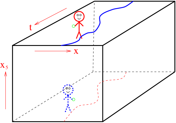
Figure 4: In the domain wall approach we start with a five dimensional lattice theory set up so that low energy fermionic states are bound to the four dimensional surfaces. Our four dimensional world arises as energy required to create excitations traveling into the fifth dimension goes to infinity.

These issues are currently a topic with lots of activity. For a recent review, see[27]. This is not an appropriate place to get involved in technical details, some of which remain unresolved. Several elegant schemes for making chiral symmetry more manifest have recently been developed. My current favorite is the “domain-wall” formulation[28], where our four dimensional world is an interface in an underlying five dimensional theory, as sketched in Fig. (4). The five dimensional quarks are given masses of order the cutoff, but the basic action is adjusted so that there are topologically stable zero mass modes bound on the surfaces of the system. At low energies in the continuum limit only these four dimensional modes are excited.

This approach works quite well for vector-like theories, with opposite chirality quarks living on opposite walls of the five dimensional theory. For chiral gauge theories, however, it is necessary to eliminate the modes on one of the two walls. It is not known how to do this in a clean way since the gauge fields do not know about the fifth dimension, and thus see both walls. Various techniques have been proposed to give a large mass to excitations on the the unwanted wall. This could be done with a Higgs coupling that becomes large on one wall; this is effectively a mirror fermion model. Another proposal involves artificially increasing the strength of the ’t Hooft vertex on the unwanted wall[29]; this involves four fermion couplings at the scale of the cutoff and is very difficult to treat rigorously.

Closely related to the domain wall approach are the “Ginsparg-Wilson’ fermionic actions, which maintain an exact, albeit somewhat more complicated, chiral symmetry[30, 31, 32]. This approach is mathematically extremely elegant, giving rise to an exact lattice version of the continuum index theorem relating zero eigenvalues of the Dirac operator with the topological index of the gauge fields. While a lattice regularization of a full chiral gauge theory such as the standard model remains elusive, we may not be far off.

12 Concluding remarks

In summary, lattice gauge theory provides the dominant framework for investigating non-perturbative phenomena in quantum field theory. The approach is currently dominated by numerical simulations, although the basic framework is potentially considerably more flexible. With the recent developments towards implementing chiral symmetry on the lattice, including domain-wall fermions, the overlap formula, and variants on the Ginsparg-Wilson relation, parity conserving theories, such as the strong interactions, are fundamentally in quite good shape.

I personally am fascinated by the chiral gauge problem. Without a proper lattice formulation of a chiral gauge theory, it is unclear whether such models make any sense as a fundamental field theories. A marvelous goal would be a fully finite, gauge invariant, and local lattice formulation of the standard model. The problems encountered with chiral gauge theory are closely related to similar issues with super-symmetry, another area that does not naturally fit on the lattice. This also ties in with the explosive activity in string theory and a possible regularization of gravity.

The other major unsolved problems in lattice gauge theory are algorithmic. Current fermion algorithms are extremely awkward and computer intensive. It is unclear why this has to be so, and may only be a consequence of our working directly with fermion determinants. One could to this for bosons too, but that would clearly be terribly inefficient. At present, the fermion problem seems completely intractable when the fermion determinant is not positive. This is of more than academic interest since interesting superconducting phases are predicted at high quark density. Similar sign problems appear in other fields, such as doped strongly coupled electron systems, thus making this problem practically quite important.

Finally, throughout history the question of “what is elementary?” continues to arise. This is almost certainly an ill posed question, with one or another approach being simpler in the appropriate context. See E. Witten’s contribution to this volume for a discussion of some of the modern equivalences. At a more mundane level, for low energy chiral dynamics we lose nothing by considering the pion as an elementary pseudo-goldstone field, while at extremely short distances string structures may become more fundamental. Quarks and their confinement may just be useful temporary constructs along the way.

Acknowledgment

This manuscript has been authored under contract number DE-AC02-98CH10886 with the U.S. Department of Energy. Accordingly, the U.S. Government retains a non-exclusive, royalty-free license to publish or reproduce the published form of this contribution, or allow others to do so, for U.S. Government purposes.

References

- [1] G. ’t Hooft, Nucl. Phys. B35, 167 (1971); G. ’t Hooft and M. Veltman, Nucl. Phys. B44, 189 (1972).
- [2] C. N. Yang and R. L. Mills, Phys. Rev. 96, 191 (1954).
- [3] H. D. Politzer, Phys. Rev. Lett. 30, 1346 (1973); D. J. Gross and F. Wilczek, Phys. Rev. Lett. 30, 1343 (1973).
- [4] J. J. Aubert et al., Phys. Rev. Lett. 33, 1404 (1974); J. E. Augustin et al., Phys. Rev. Lett. 33, 1406 (1974).
- [5] S. Coleman, in C75-07-11.13 Print-77-0088 (HARVARD) Lectures delivered at Int. School of Subnuclear Physics, Ettore Majorana, Erice, Sicily, Jul 11-31, 1975; published in Erice Subnucl. Phys. 1975:297 (QCD161:I65:1975:PT.A).
- [6] A. A. Belavin, A. M. Polyakov, A. S. Shvarts and Y. S. Tyupkin, Phys. Lett. B 59 (1975) 85.
- [7] F. J. Wegner, J. Math. Phys. 12, 2259 (1971).
- [8] J. Smit, UCLA Thesis, pp. 24-26 (1974).
- [9] R. Balian, J. M. Drouffe and C. Itzykson, Phys. Rev. D10, 3376 (1974); Phys. Rev. D11, 2098 (1975); Phys. Rev. D11, 2104 (1975).
- [10] S. Coleman and E. Weinberg, Phys. Rev. D7, 1888 (1973).
- [11] M. Creutz, Phys. Rev. Letters (in press, 2004), arXiv:hep-ph/0312225.
- [12] D. E. Groom et al., European Physical Journal C15, 1 (2000).
- [13] M. Creutz, L. Jacobs and C. Rebbi, Phys. Rev. Lett. 42, 1390 (1979).
- [14] F. Karsch, Nucl. Phys. Proc. Suppl. 83, 14 (2000) [hep-lat/9909006].
- [15] C. Bernard et al. [MILC Collaboration], Phys. Rev. D55, 6861 (1997) [hep-lat/9612025].
- [16] M. Creutz, Phys. Rev. Lett. 81 (1998) 3555 [arXiv:hep-lat/9806037].
- [17] M. Creutz, Int. J. Mod. Phys. C 14 (2003) 1027 [arXiv:hep-lat/0212034].
- [18] F. Wilczek, Nucl. Phys. A663, 257 (2000) [hep-ph/9908480].
- [19] J. S. Bell and R. Jackiw, Nuovo Cim. A 60 (1969) 47.
- [20] S. L. Adler, Phys. Rev. 177 (1969) 2426.
- [21] S. L. Adler and W. A. Bardeen, Phys. Rev. 182 (1969) 1517.
- [22] G. ’t Hooft, Phys. Rev. Lett. 37 (1976) 8.
- [23] G. ’t Hooft, Phys. Rev. D 14 (1976) 3432 [Erratum-ibid. D 18 (1978) 2199].
- [24] E. Eichten and J. Preskill, Nucl. Phys. B 268 (1986) 179.
- [25] I. Montvay, Phys. Lett. B 199 (1987) 89.
- [26] I. Montvay, Nucl. Phys. Proc. Suppl. 29BC (1992) 159 [arXiv:hep-lat/9205023].
- [27] M. Creutz, Rev. Mod. Phys. 73, 119 (2001) [arXiv:hep-lat/0007032].
- [28] D. B. Kaplan, Phys. Lett. B 288 (1992) 342 [arXiv:hep-lat/9206013].
- [29] M. Creutz, M. Tytgat, C. Rebbi and S. S. Xue, Phys. Lett. B 402 (1997) 341 [arXiv:hep-lat/9612017].
- [30] H. Neuberger, Phys. Lett. B417 (1998) 141; H. Neuberger, Phys. Lett. B427 (1998) 353; R. Narayanan and H. Neuberger, Phys. Lett. B302 (1993) 62; Phys. Rev. Lett. 71 (1993) 3251; Nucl. Phys. B412 (1994) 574; Nucl. Phys. B443 (1995) 305.
- [31] P. Hernandez, K. Jansen and M. Luscher, Nucl. Phys. B 552 (1999) 363; M. Luscher, Commun. Math. Phys. 85 (1982) 39.
- [32] P. H. Ginsparg and K. G. Wilson, Phys. Rev. D 25 (1982) 2649.