Blocking from continuum and monopoles in gluodynamics

Abstract

We review the method of blocking of topological defects from continuum used as a non–perturbative tool to construct effective actions for these defects. The actions are formulated in the continuum limit while the couplings of these actions can be derived from simple observables calculated numerically on lattices with a finite lattice spacing. We demonstrate the success of the method in deriving the effective actions for Abelian monopoles in the pure SU(2) gauge models in an Abelian gauge. In particular, we discuss the gluodynamics in three and four space–time dimensions at zero and non–zero temperatures. Besides the action the quantities of our interest are the monopole density, the magnetic Debye mass and the monopole condensate.

I Introduction

The blocking from continuum (BFC) is a well–known tool to construct the ”perfect actions” for lattice field theories ref:BFC . By definition a perfect lattice action does not depend on the cut-off parameter which is usually associated with the finite lattice spacing. The cut-off dependence provides a systematic error in the lattice observables which is of the order of the lattice spacing for the standard Wilson action. The various improvement schemes ref:improvement are used to decrease the cut–off influence on the lattice results, and the BFC method ref:BFC is one of the practically useful tools used in the lattice simulations nowadays.

Although the main idea of introducing the BFC is to reduce the systematic errors in the numerical simulations, a philosophically similar method can be applied to various topological defects. As a result one can derive effective actions for the defects in the continuum limit using results of the lattice simulations obtained on lattices with finite lattice spacings. This short review is devoted to a demonstration of success of the method applied to the Abelian monopoles in the lattice gluodynamics in three dimensions (where the monopoles are instanton–like objects) and in four dimensions (where the monopoles are particle–like defects) following Refs. ref:3D ; ref:4Dhigh ; ref:4D . One should stress from the very beginning that the method is quite general and is not limited to the lattice monopoles only.

First, let us remind basics of the BFC method for field degrees of freedom. A simplest way to associate, say, a continuum free fermion field, $\psi(x)$, with a lattice fermion field, $\Psi_{s}$, is ref:BFC :

$$\Psi_{s}=\int_{C_{s}}\mbox{d}^{4}x\,\psi(x)\,,\quad{\bar{\Psi}}_{s}=\int_{C_{s}}\mbox{d}^{4}x\,{\bar{\psi}}(x)\,,$$ (1)

where the integration is carried out over the lattice hypercube, $C_{s}$, centered in the lattice point $s$ (we will come to the precise definition of $C_{s}$ later). Equations (1) can then be inserted into the partition function as the $\delta$–function constraint. To complete the procedure of blocking the continuum fields $\psi(x)$ should be integrated out leaving us with the partition function depending solely on the lattice fields $\Psi_{s}$. Similar relations can also be written for the gauge fields $etc.$. We refer a reader interested in the blocking of fields to the original articles switching at this point to the blocking of the topological defects.

Suppose, that we have a (gauge) model which describes topological defects, say, for definiteness, monopoles. In four space–time dimensions (4D) the monopole is a particle-like object ($i.e.$, its trajectory is line–like), and the monopole charge is quantized and conserved ($i.e.$, the monopole trajectories are closed loops). Obviously, basic requirements to the topological BFC procedure should be the following: (i) the procedure should provide us with the configuration of the lattice monopole currents for a given configuration of the continuum monopole currents; (ii) the lattice monopole currents must be closed; (iii) the lattice magnetic charge for such monopoles must be quantized. We show below that one may write a blocking relation similar (but, in general, not identical) to Eq. (1), which associates the lattice and the continuum monopole charges and preserves their basic properties. We insert this relation into the partition function in a form of the $\delta$–function constraint, integrate out the continuum degrees of freedom and get the lattice model which contains only the lattice monopole currents. Using the BFC method one can also get analytical formulae for various lattice observables expressed through the parameters of the continuum model. A comparison of the numerical data for such observables with the corresponding analytical expressions provides us with the parameters of the monopole action in the continuum. Note that the blocking of the topological defects from the continuum to the lattice is similar to ideas of Refs. ref:Fujimoto ; ExtendedMonopoles which discussed theoretically the blocking of the monopoles from fine lattices to coarse lattices.

Below we describe how the method works for the Abelian monopoles in SU(2) gluodynamics. Many monopole observables have been calculated numerically Review . Even an almost perfect monopole action on the lattice has been determined (in a truncated form) using an inverse Monte–Carlo method ref:NumericalMonopoleAction . However, the correctness of the truncation, or, in other words, the correct form of the perfect lattice action is not known. The BFC method allows us to find couplings of the (truncated) perfect monopole action in the continuum, estimate the error of the truncation, and to obtain certain non–perturbative quantities. Our interest in the physics of the Abelian monopoles in the non–Abelian pure gauge theories is stimulated by the relation of the monopole dynamics to the one of the most important problems of QCD, the confinement of color. One popular approach to this problem is the so–called dual superconductor mechanism DualSuperconductor (for a review of another interesting approach, the vacuum correlator method, see Ref. AYuReview ). The key role in the dual superconductor mechanism is played by Abelian monopoles which are identified with the help of the Abelian projection method AbelianProjections . The basic idea behind the Abelian projections is to fix partially the non–Abelian gauge symmetry up to an Abelian subgroup. For SU(N) gauge theories the residual Abelian symmetry group is compact since the original non-Abelian group is compact as well. The Abelian monopoles arise naturally due to the compactness of the residual gauge subgroup.

The Abelian monopoles are not present in QCD from the beginning: they are not solutions to the classical equation of motion of this theory. However, the monopoles may be considered as effective degrees of freedom which are responsible for confinement of quarks. According to the numerical results MonopoleCondensation the monopoles are condensed in the low temperature (confinement) phase. The condensation of the monopoles leads to formation of the chromoelectric string due to the dual Meissner effect. As a result the fundamental sources of chromoelectric field, quarks, are confined by the string. The importance of the Abelian monopoles is also stressed by the existence AbelianDominance of the Abelian dominance phenomena which were first observed in the lattice $SU(2)$ gluodynamics: the monopoles in the so-called Maximal Abelian projection MaA make a dominant contribution to the zero temperature string tension.

In the deconfinement phase (high temperatures) the monopoles are not condensed and the quarks are liberated. This does not mean, however, that monopoles do not play a role in non-perturbative physics. It is known that in the deconfinement phase the vacuum is dominated by static monopoles (which run along the ”temperature” direction in the Euclidean theory) while monopoles running in spatial directions are suppressed. The static monopoles should contribute to the ”spatial string tension” – a coefficient in front of the area term of large spatial Wilson loops. And, according to numerical simulations in the deconfinement phase AbelianDominanceT , the monopoles make a dominant contribution to the spatial string tension. Thus, the monopoles may play an important role not only in the low temperatures but also in the high temperature phase.

We refer a reader to Ref. Review for a review on the Abelian projections and the dual superconductor models in non-Abelian gauge theories.

The structure of the paper is as follows. In Section II we describe the BFC method in the simplest three–dimensional (3D) case. Assuming that in the continuum the monopole action is of the Coulomb form we derive the lattice monopole action and the lattice density of the (squared) monopole charges. In Section III we apply the BFC procedure to the Abelian monopoles in the four–dimensional SU(2) gauge theory. Assuming that the monopoles are described by the dual Ginzburg–Landau model one can get an analytical form for the quadratic monopole action on the lattice.

Then in Section IV we compare the analytical formulae with the corresponding numerical data obtained in the three dimensional SU(2) gauge model. As a result we get the density of the monopoles and the monopole contribution to the magnetic screening length in the continuum limit of this model. We show that the results obtained with the help of the BFC method are in agreement with the results of other (independent) calculations. In Section V we apply the 3D BFC method to the temporal components of the monopole currents in SU(2) gauge model in the four space–time dimensions at high temperature. This gives us a numerical value of the product of the Abelian magnetic screening mass and the monopole density in the continuum model. The self–consistency check shows that the dynamics of the static monopole currents can be described by the Coulomb gas model starting from the temperatures $T\gtrsim 2.5T_{c}$.

Finally, in Section VI we get the value of the monopole condensate in the continuum using the 4D BFC method. This value is in agreement with the results obtained with the help of other methods. Our conclusion in presented in the last Section.

II Blocking in three dimensions

It is instructive to start the description of the BFC method from the simplest three–dimensional case. In three dimensions the Abelian monopoles are point–like objects characterized by a position, $x$, and the magnetic charge, $q$ (measured in units of a fundamental magnetic charge, $g_{M}$). The simplest model possessing the monopoles is the 3D compact quantum electrodynamics (cQED₃)in which the monopole action is given by the $3D$ Coulomb gas model Polyakov :

$${\cal Z}=\sum\limits_{N=0}^{\infty}\frac{\zeta^{N}}{N!}\Biggl{[}\prod\limits^{N}_{a=1}\int\mbox{d}^{3}x^{(a)}\sum\limits_{q_{a}=\pm 1}\Biggr{]}\exp\Bigl{\{}-\frac{g^{2}_{M}}{2}\sum\limits_{\stackrel{{\scriptstyle a,b=1}}{{a\neq b}}}^{N}q_{a}q_{b}\,D(x^{(a)}-x^{(b)})\Bigr{\}}\,.$$ (2)

The Coulomb interaction in Eq.(2) is represented by the inverse Laplacian $D$: $-\partial^{2}_{i}D(x)=\delta^{(3)}(x)$, and the latin indices $a,b$ label different monopoles. To get analytical expressions below we make a standard assumption that the density of the monopoles is low. The monopole charges therefore are restricted by the condition $|q_{a}|\leq 1$ which means that the monopoles do not overlap. The average monopole density $\rho$ is controlled by the fugacity parameter $\zeta$, giving $\rho=2\zeta$ in the leading order of the dilute gas approximation Polyakov

The magnetic charges in the Coulomb gas (2) are screened: at large distances the two–point charge correlation function is exponentially suppressed, $\langle\rho(x)\rho(y)\rangle\sim\exp\{-|x-y|/\lambda_{D}\}$. Here $\lambda_{D}$ is the Debye screening length Polyakov ,

$$\lambda_{D}=\frac{1}{g_{M}\sqrt{\rho}}\,.$$ (3)

The three dimensional Debye screening length corresponds to a magnetic screening in four dimensions. Below we choose the vacuum expectation value of the continuum monopole density $\rho$ and the Debye screening length $\lambda_{D}$ as suitable parameters of the continuum model (instead of $g_{M}$ and $\zeta$).

Next, let us consider a lattice with a finite lattice spacing $b$ which is embedded in the continuum space-time. The cells of the lattice are defined as follows:

$$C_{s}=\Biggl{\{}b\Bigl{(}s_{i}-\frac{1}{2}\Bigr{)}\leq x_{i}\leq b\Bigl{(}s_{i}+\frac{1}{2}\Bigr{)}\,,\quad i=1,2,3\Biggr{\}}\,,$$ (4)

where $s_{i}$ is the lattice dimensionless coordinate and $x_{i}$ corresponds to the continuum coordinate.

The basic idea of the BFC method is to treat each lattice 3D cell as a ”detector” of the magnetic charges of the continuum monopoles. The relation between the lattice magnetic charge $k_{s}$ and the density of the continuum monopoles $\rho(x)$ is

$$k_{s}=\int\limits_{C_{s}}\mbox{d}^{3}x\,\rho(x)\,,\qquad\rho(x)=\sum_{a}q_{a}\,\delta^{(a)}(x-x^{(a)})\,,$$ (5)

see an illustration in Figure 1.

Figure 1: Blocking of the continuum monopoles to the lattice in three dimensions. The charge of the lattice monopole in the cube ${\cal C}$ is given by the total magnetic charge of the continuum monopoles inside this cube.

The fluctuations of the monopole charges of the lattice cells must depend on the properties of the continuum monopoles. As a result, the lattice observables – such as the vacuum expectation value of the lattice monopole density – must carry information about dynamics of the continuum monopoles. The observables should depend not only on the size of the lattice cell, $b$, but also on the features of the continuum model which describes the monopole dynamics.

It is worth stressing the difference between the continuum and the lattice monopoles: the continuum monopoles are fundamental point–like objects while the lattice monopoles are associated with the finite–sized lattice cells with non-vanishing total magnetic charge.

According to definitions (5), the lattice monopole charge shares similar properties to the continuum monopole charge. The monopole charge $k_{s}$ is quantized, $k_{s}\in{Z\!\!\!Z}$, and it is conserved in the three-dimensional sense:

$$\sum\limits_{s\in\Lambda}k_{s}\equiv\int\limits_{V}\mbox{d}^{3}x\,\rho(x)=0\,,$$ (6)

if the continuum charge is conserved. Here $\Lambda$ and $V$ denote the lattice and the continuum volume occupied by the lattice, respectively. In other words, the total magnetic charge of the lattice monopole configuration is zero on a finite lattice with periodic boundary conditions.

In next two subsections we follow Ref. ref:3D presenting in the BFC approach the simplest quantities characterizing the lattice monopoles: the monopole action $S_{mon}(k)$ and the vacuum expectation value of the squared magnetic charge, $\langle k^{2}_{s}\rangle$.

II.1 Monopole action in 3D

To derive the lattice monopole action we substitute the unity,

$$1=\sum_{k(\Lambda)\in{Z\!\!\!Z}}\prod_{s\in\Lambda}\delta_{\Lambda}\Bigl{(}k_{s}-\int\limits_{C_{s}}\mbox{d}^{3}x\,\rho(x)\Bigr{)}\,,$$ (7)

into Eq.(2). Here $\sum_{k(\Lambda)\in{Z\!\!\!Z}}\equiv\prod_{s\in\Lambda}\sum_{k_{s}\in{Z\!\!\!Z}}$ and $\delta_{\Lambda}$ stands here for the Kronecker symbol ($i.e.$, lattice $\delta$–function). We get

$${\cal Z} = \sum_{k(\Lambda)\in{Z\!\!\!Z}}\sum\limits_{N=0}^{\infty}\frac{\zeta^{N}}{N!}\Biggl{[}\prod\limits^{N}_{a=1}\int\mbox{d}^{3}x^{(a)}\sum\limits_{q_{a}=\pm 1}\Biggr{]}\int\limits^{\pi}_{-\pi}{\cal D}_{\Lambda}h\int{\cal D}\chi\exp\Biggl{\{}-\int\mbox{d}^{3}x\Bigl{[}\frac{1}{2g^{2}_{M}}{\bigl{(}\partial_{i}\chi(x)\bigr{)}}^{2}$$ (8)

$$+i\rho(x)\Bigl{(}\chi(x)-\sum_{s\in\Lambda}\theta_{s}(x)h_{s}\Bigr{)}+i\sum_{s\in\Lambda}k_{s}h_{s}\Bigr{]}\Biggr{\}}\,,$$

where we have introduced two additional integrations over the continuum field $\chi$ and the compact lattice field $h$ to represent the inverse Laplacian in Eq.(2) and the Kronecker symbol in Eq.(7), respectively. The subscript $\Lambda$ in ${\cal D}_{\Lambda}h$ indicates that the integration is going over the lattice fields $h$. The representative function of the $s^{\mathrm{th}}$ lattice cell is denoted as $\theta_{s}$:

$$\theta_{s}(x)=\left\{\begin{array}[]{ll}1\,,&x\in C_{s}\,,\\ 0\,,&\mbox{otherwise}\,.\\ \end{array}\right.$$ (11)

Summing over the monopole position according to Ref. Polyakov , expanding the cosine function over the small fluctuations in the fields $\chi$ and $h$, and integrating over these fields we get the monopole action:

$$S^{tree}_{mon}(k)=\frac{1}{4\zeta b^{3}}\sum_{s,s^{\prime}}k_{s}\,{\cal F}_{s,s^{\prime}}k_{s^{\prime}}\,.$$ (12)

where

$${\cal F}^{-1}_{s,s^{\prime}} = \delta_{s,s^{\prime}}-m^{2}_{D}b^{2}{\cal G}_{s,s^{\prime}}\,,$$ (13)

$${\cal G}_{s,s^{\prime}} = \frac{1}{b^{5}}\int\mbox{d}^{3}x\int\mbox{d}^{3}y\theta_{s}(x)\,D_{m_{D}}(x-y)\,\theta_{s^{\prime}}(y)\,,$$ (14)

and $D_{m_{D}}$ is the scalar propagator for a massive particle, $(-\partial^{2}_{i}+m^{2})D_{m}(x)=\delta^{(3)}(x)$, with the Debye mass $m=m_{D}\equiv\lambda^{-1}_{D}$. Note that the lattice operators ${\cal F}$ and ${\cal G}$ are dimensionless quantities.

In the infinite lattice case Eq. (13) can be rewritten as follows

$${\cal F}_{s,s^{\prime}}=\int\limits^{\pi}_{-\pi}\frac{\mbox{d}^{3}u}{(2\pi)^{3}}\,{\Biggl{[}\sum_{r(\Lambda)\in{Z\!\!\!Z}}\sum_{i=1}^{3}\frac{4\,\sin^{2}(u_{i}/2)}{(\vec{u}+2\pi\vec{r})^{2}+\mu^{2}}\,\prod^{3}_{\stackrel{{\scriptstyle j=1}}{{j\neq i}}}{\Biggl{(}\frac{2\sin(u_{j}/2)}{u_{j}+2\pi r_{j}}\Biggr{)}}^{2}\Biggr{]}}^{-1}\cdot e^{i(s-s^{\prime},u)}\,.$$ (15)

where

$$\mu=b/\lambda_{D}\,,$$ (16)

The finite–volume expression for the monopole action can be obtained from Eq.(15) by the standard substitution:

$$u_{i}\to\frac{2\pi k_{i}}{L_{i}}\,,\qquad k=0\,,1\,,\dots L_{i}-1\,,\qquad\int\limits^{\pi}_{-\pi}\frac{\mbox{d}u_{i}}{2\pi}\to\frac{1}{L_{i}}\sum\limits_{k_{i}=0}^{L_{i}-1}\,,$$ (17)

where $L_{i}$ is the lattice size in $i^{\mathrm{th}}$ direction.

In the infinite–volume case the lattice operator ${\cal F}_{s,s^{\prime}}$ depends only on the dimensionless quantity $\mu$, Eq.(16), which is the ratio of the monopole size $b$ and the Debye screening length, Eq.(3). The form of the operator ${\cal F}$ is qualitatively different in the limits of small and large $\mu$. Namely, the leading contribution to the monopole action is given by the mass (Coulomb) terms for small (large) lattice monopoles ref:3D :

$$S_{mon}(k)=\left\{\begin{array}[]{lll}\frac{1}{4\rho}\cdot\frac{1}{b^{3}}\cdot\sum\limits_{s}k^{2}_{s}+\cdots\,,&b\ll\lambda_{D}\,;\\ \frac{1}{\rho\,\lambda_{D}}\cdot\frac{1}{b^{2}}\cdot\sum\limits_{s,s^{\prime}}k_{s}\,D_{s,s^{\prime}}\,k_{s^{\prime}}+\cdots\,,&b\gg\lambda_{D}\,,\end{array}\right.$$ (20)

where $D_{s,s^{\prime}}$ is the inverse Laplacian on the lattice. Thus the Debye length $\lambda_{D}$ sets a scale for the lattice monopole size (or, better to say, for the size of the lattice cell) which characterizes different behavior of the monopole action.

II.2 Squared monopole density in 3D

The simplest quantity characterizing the lattice monopoles is the monopole density $\rho_{latt}(b)$ measured in the lattice units

$$\rho_{latt}(b)=\frac{1}{L^{3}}\,\langle\sum_{s\in\Lambda}|k_{s}|\rangle\,,$$ (21)

where $L$ is the lattice size in units of $b$. However, analytically it is more easier to calculate the density of the squared monopole charges,

$$\langle k^{2}(b)\rangle=\frac{1}{L^{3}}\,\langle\sum_{s\in\Lambda}k^{2}(s)\rangle\,,$$ (22)

which has a similar physical meaning to the monopole density.

Using Eq.(5) the lattice density (22) can be written in the continuum theory as follows:

$$\langle k^{2}(b)\rangle=\int_{C_{s}}\mbox{d}^{3}x\int_{C_{s}}\mbox{d}^{3}y\,\langle\rho(x)\,\rho(y)\rangle\,,$$ (23)

where the lattice site $s$ is fixed and the average is taken in the Coulomb gas of the magnetic monopoles described by the partition function (2).

The correlator of the monopole densities, $\langle\rho(x)\,\rho(y)\rangle$, is well known from Ref. Polyakov . Introducing the source for the magnetic monopole density, $J$, Eq.(23) can be rewritten as follows:

$$\langle k^{2}\rangle=-\int_{C_{s}}\mbox{d}^{3}x\int_{C_{s}}\mbox{d}^{3}y\,\frac{\delta^{2}}{\delta J(x)\,\delta J(y)}<\exp\Bigl{\{}i\int\mbox{d}^{3}z\rho(z)\,J(z)\Bigr{\}}>{\Biggl{|}}_{J=0}\,.$$ (24)

Then we repeat the transformations in the previous Section which led us to Eqs.(12),(15). Integrating over quadratic fluctuations of the field $\chi$ we get in the leading order

$$\langle\rho(x)\,\rho(y)\rangle=\rho\,\Bigl{[}\delta^{(3)}(x-y)-m^{2}_{D}D_{m_{D}}(x-y)\Bigr{]}\,.$$ (25)

Substituting Eq.(25) in Eq.(23) and taking the integrals over the cell $C_{s}$ we get

$$\langle k^{2}\rangle=\rho\,b^{3}\,{({\cal F}^{-1})}_{0,0}(\mu)\,,$$ (26)

where the inverse matrix ${\cal F}_{s,s^{\prime}}$ is given by Eq.(13). Equation (26) establishes a direct relation between the density of the squared monopole charges and the monopole action (12) in a leading approximation of the dilute gas.

The squared monopole charge satisfies the following:

$$\langle k^{2}\rangle=\left\{\begin{array}[]{ll}C_{1}\,\rho\,\lambda_{D}\,b^{2}\cdot\left[1+O\left({\left(\lambda_{D}/b\right)}^{2}\right)\right]\,,&\quad b\gg\lambda_{D}\,,\\ \rho\,b^{3}\cdot\left[1+C_{2}\,\rho\,{(b/\lambda_{D})}^{2}\,+O\left({\left(b/\lambda_{D}\right)}^{4}\right)\right]\,,&\quad b\ll\lambda_{D}\,.\end{array}\right.$$ (29)

where $C_{1}\approx 2.94$ and $C_{2}\approx 0.148$ in the infinite lattice case.

Equation (29) can qualitatively be understood as follows. In the small $b$ region the density of the squared lattice monopole charges is equal to the density of the continuum monopoles times the volume of the cell. This is natural, since the smaller volume of the lattice cell ($Vol=b^{3}$) the smaller chance for two monopoles to be located at the same cell. Therefore each cell predominantly contains not more that one monopole, which leads to the relation $k^{2}_{s}=|k_{s}|=0,1$. As a result we get $\langle k^{2}\rangle\to\rho_{latt}(b)\to\rho\,b^{3}$ in the limit $b\to 0$. In the large-$b$ region correlations between monopoles start to play a role. The monopoles separated from the boundary of the cell by a distance larger than $\lambda_{D}$, do not contribute to $\langle k^{2}\rangle$. Consequently, the $b^{3}$ proportionality for the random gas turns into $\lambda_{D}b^{2}$ in the Coulomb gas and we get $\langle k^{2}\rangle\sim\rho\,\lambda_{D}\,b^{2}$.

Finally, let us mention interesting relations between the density of the small– and large– sized monopoles and the coefficients in front of, respectively, the Coulomb terms and the mass terms of the monopole action, Eqs. (20),(29):

$$C(b)=\frac{C_{1}}{\langle k^{2}(b)\rangle}\,,\quad b\gg\lambda_{D}\,,\quad\mbox{and}\quad M(b)=\frac{1}{4\,\langle k^{2}(b)\rangle}\,,\quad b\ll\lambda_{D}\,.$$ (30)

III Blocking in four dimensions

In four space–time dimensions the monopole trajectories are closed loops. Let us superimpose a cubic lattice with the lattice spacing $b$ on a particular configuration of the monopoles. Each of the (oriented) lattice $3D$ cells can be characterized by an integer magnetic charge it contains. Thus we can relate the continuum configuration of the monopoles to the lattice configuration. The three-dimensional cubes are defined as follows:

$$C_{s,\mu}=\Biggl{\{}b\Bigl{(}s_{\nu}-\frac{1}{2}\Bigr{)}\leq x_{\nu}\leq b\Bigl{(}s_{\nu}+\frac{1}{2}\Bigr{)}\,\,\mbox{for}\,\,\nu\neq\mu\,;\,\,\mbox{and}\,\,x_{\mu}=bs_{\mu}\Biggr{\}}\,,$$ (31)

where $s_{\nu}$ is the dimensionless lattice coordinate of the lattice cube $C_{s,\mu}$ and $x_{\nu}$ is the continuum coordinate. The direction of the $3D$ cube in the $4D$ space is defined by the Lorentz index $\mu$.

The monopole charge $K_{C}$ inside the lattice cube $C_{s,\mu}$ is equal to the total charge of the continuum monopoles, $k$, which pass through this cube. Geometrically, the total monopole corresponds to the linking number between the cube $C$ and the monopole trajectories, $k$ (an illustration is presented in Fig. 2).

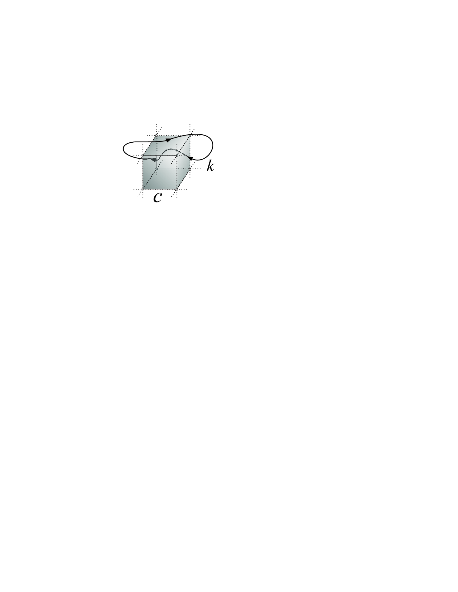
Figure 2: Blocking of the continuum monopoles to the lattice in four dimensions. The lattice monopole charge is equal to the linking number of the monopole trajectory, $k$, with the surface of the three–dimensional cube ${\cal C}$.

The mutual orientation of the cube and the monopole trajectory is obviously important. The corresponding mathematical expression for the monopole charge $K_{C}$ inside the cube $C$ is a generalization of the Gauss linking number to the four dimensional space–time ref:4D :

$$K_{C}(k)\equiv{I\!\!L}(\partial C,k) = \frac{1}{2}\int\!\mbox{d}^{4}x\int\!\mbox{d}^{4}y\,\epsilon_{\mu\nu\alpha\beta}\,\Sigma^{\partial C}_{\mu\nu}(x)\,k_{\alpha}(y)\,\partial_{\beta}{\cal D}^{(4)}(x-y)$$ (32)

$$= \frac{1}{4\pi^{2}}\int\mbox{d}^{4}x\int\mbox{d}^{4}y\,\epsilon_{\mu\nu\alpha\beta}\,\Sigma^{\partial C}_{\mu\nu}(x)\,k_{\alpha}(y)\,\frac{{(x-y)}_{\beta}}{{|x-y|}^{4}}\,.$$

Here the function $\Sigma^{\partial C}_{\mu\nu}(x)$ is the two–dimensional $\delta$–function representing the boundary $\partial C$ of the cube $C$. In general form it can be written as follows:

$$\Sigma_{\alpha\beta}(x)=\int_{\Sigma}\mbox{d}\tau_{1}\mbox{d}\tau_{2}\,\frac{x_{[\alpha,}(\vec{\tau})}{\partial\tau_{a}}\frac{x_{\beta]}(\vec{\tau})}{\partial\tau_{b}}\,\delta^{(4)}[x-\tilde{x}(\vec{\tau})]\,,$$ (33)

where the four dimensional vector $\tilde{x}(\vec{\tau})$ parameterizes the position of the two–dimensional surface $\Sigma$. The function ${\cal D}^{(4)}$ in Eq. (32) is the inverse Laplacian in four dimensions, $\partial^{2}_{\mu}{\cal D}^{(4)}(x)=\delta^{(4)}(x)$. It is obvious that the lattice currents $K_{s,\mu}$ are closed

$$\partial^{\prime}K=0\,,$$ (34)

due to the conservation of the continuum monopole charge, $\partial_{\mu}k_{\mu}=0$. In Eq. (34) the symbol $\partial^{\prime}$ denotes the backward derivative on the lattice.

Following Ref. ref:4D we derive the lattice monopole action starting from a particular model for the monopole currents. We consider the model dual superconductor the partition function of which can be written as a sum over the monopole trajectories:

$${\cal Z}_{mon}=\int\Sigma{\cal D}k\int{\cal D}B\,\exp\Bigl{\{}-\int\mbox{d}^{4}x\,\Bigl{[}\frac{1}{4g^{2}}F^{2}_{\mu\nu}+ik_{\mu}(x)B_{\mu}(x)\Bigr{]}-S_{int}(k)\Bigr{\}}\,,$$ (35)

where $F_{\mu\nu}=\partial_{\mu}B_{\nu}-\partial_{\nu}B_{\mu}$ is the field stress tensor of the dual gauge field $B_{\mu}$, and $S_{int}(k)$ is the action of the closed monopole currents $k$,

$$k_{\mu}(x)=\oint\mbox{d}\tau\,\frac{\partial{\tilde{x}}_{\mu}(\tau)}{\partial\tau}\,\delta^{(4)}[x-\tilde{x}(\tau)]\,.$$ (36)

Here the $4D$ vector function ${\tilde{x}_{\mu}}(\tau)$ defines the trajectory of the monopole current. In Eq. (35) the integration is carried out over the dual gauge fields and over all possible monopole trajectories (the sum over disconnected parts of the monopole trajectories is also implicitly assumed).

The action in Eq. (35) contains three parts: the kinetic term for the dual gauge field, the interaction of the dual gauge field with the monopole current and the self–interaction of the monopole currents. The integration over the monopole trajectories gives the Lagrangian of the dual Abelian Higgs model ref:suzuki:maedan :

$${\cal Z}_{mon}\propto{\cal Z}_{DAHM}=\int{\cal D}\Phi\int{\cal D}B\,\exp\Bigl{\{}-\int\mbox{d}^{4}x\,\Bigl{[}\frac{1}{4g^{2}}F^{2}_{\mu\nu}+\frac{1}{2}|(\partial_{\mu}+iB_{\mu})\Phi|^{2}+V(\Phi)\Bigr{\}}\,,$$ (37)

where $\Phi$ is a complex monopole field. The self–interactions of the monopole trajectories described by the action $S_{int}$ in Eq. (35) lead to the self–interaction of the monopole field $\Phi$ described by the potential term $V(\Phi)$ in Eq. (37). This model is nothing but the usual Ginzburg–Landau model written for the dual fields $\Phi$ and $B_{\mu}$.

Similarly to the three dimensional case let us rewrite the dual superconductor model (37) in terms of the lattice currents $K_{C}$, Eq. (32). To this end we insert the unity,

$$1=\sum\limits_{K_{C}\in{Z\!\!\!Z}}\,\prod\limits_{C}\delta\Bigl{(}K_{C}-{I\!\!L}(\partial C,k)\Bigr{)}\,,$$ (38)

into the partition function (35) (here $\delta$ represents the Kronecker symbol). Then we integrate the continuum degrees of freedom, $k_{\mu}$ and $B_{\mu}$, getting the partition function in terms of the lattice charges $K_{C}$. The simplest way to do so is to represent the product of the Kronecker symbols in Eq. (38) in terms of the integrals,

$$1=\sum\limits_{K_{C}\in{Z\!\!\!Z}}\,\Bigl{[}\prod_{C}\int\limits^{\infty}_{-\infty}\mbox{d}\theta_{C}\Bigr{]}\,\exp\Bigl{\{}i\sum_{C}\theta_{C}\,K_{C}-i\int\mbox{d}^{4}x\,k_{\mu}(x){\tilde{B}}_{\mu}(\theta;x)\Bigr{\}}\,,$$ (39)

where

$${\tilde{B}}_{\mu}(\theta;x)=\frac{1}{2}\int\!\mbox{d}^{4}y\,\epsilon_{\mu\nu\alpha\beta}\,\partial_{\nu}{\cal D}^{(4)}(x-y)\,\sum\limits_{C}\theta_{C}\,\Sigma^{\partial C}_{\alpha\beta}(y)\,.$$ (40)

To derive Eqs. (39),(40) from Eq. (38) we have used relation (32).

Substituting Eq. (39) into Eq. (35) we get:

$${\cal Z}_{mon} = \int\Sigma{\cal D}k\int{\cal D}B\,\sum\limits_{K_{C}\in{Z\!\!\!Z}}\,\Bigl{[}\prod_{C}\int\limits^{\infty}_{-\infty}\mbox{d}\theta_{C}\Bigr{]}\,\exp\Bigl{\{}i\sum_{C}\theta_{C}\,K_{C}$$ (41)

$$-\int\mbox{d}^{4}\Bigl{[}\frac{1}{4g^{2}}F^{2}_{\mu\nu}+ik_{\mu}(x)\Bigl{(}B_{\mu}(x)+{\tilde{B}}_{\mu}(\theta;x)\Bigr{)}\Bigr{]}-S_{int}(k)\Bigr{\}}\,.$$

One can see that the substitution of the unity (39) effectively shifts the gauge field in the interaction term with the monopole current, $B_{\mu}\to B_{\mu}+{\tilde{B}}_{\mu}$. Therefore the integration over the monopole trajectories, $k_{\mu}$, in Eq. (41) is very similar to the integration which relates Eq. (35) and Eq. (37). Thus, we get:

$${\cal Z}_{mon}\propto{\cal Z}_{DAHM} = \int{\cal D}\Phi\int{\cal D}B\,\sum\limits_{K_{C}\in{Z\!\!\!Z}}\,\Bigl{[}\prod_{C}\int\limits^{\infty}_{-\infty}\mbox{d}\theta_{C}\Bigr{]}\,\exp\Bigl{\{}i\sum_{C}\theta_{C}\,K_{C}$$ (42)

$$-\int\mbox{d}^{4}x\Bigl{[}\frac{1}{4g^{2}}F^{2}_{\mu\nu}+\frac{1}{2}\Bigl{|}\Bigl{[}\partial_{\mu}+i\Bigl{(}B_{\mu}(x)+{\tilde{B}}_{\mu}(\theta;x)\Bigr{)}\Bigr{]}\Phi\Bigr{|}^{2}+V(\Phi)\Bigr{]}\Bigr{\}}\,.$$

Next we rewrite the continuum dual superconductor model in terms of the lattice monopole currents, $K$:

$${\cal Z}_{DAHM}=\sum\limits_{K_{x,\mu}\in{Z\!\!\!Z}}\,e^{-S_{mon}(K)}\,,$$ (43)

where the monopole action is defined via the lattice Fourier transformation:

$$e^{-S_{mon}(K)}=\int\limits^{\infty}_{-\infty}{\cal D}\theta_{C}\,\exp\Bigl{\{}-{\tilde{S}}(\theta)+i(\theta,K)\Bigr{\}}\,.$$ (44)

Here the action ${\tilde{S}}(\theta)$ of the compact lattice fields $\theta$ is expressed in terms of the dual Abelian Higgs model in the continuum:

$$e^{-{\tilde{S}}(\theta)}\!=\!\int\!\!{\cal D}\Phi\int\!\!{\cal D}B\,\exp\Bigl{\{}-\!\!\int\!\mbox{d}^{4}x\Bigl{[}\frac{1}{4g^{2}}F^{2}_{\mu\nu}+\frac{1}{2}\Bigl{|}\Bigl{[}\partial_{\mu}+i\Bigl{(}B_{\mu}+{\tilde{B}}_{\mu}(\theta)\Bigr{)}\Bigr{]}\Phi\Bigr{|}^{2}+V(\Phi)\Bigr{]}\Bigr{\}}\,.$$ (45)

An exact integration over the monopole, $\Phi$, and dual gauge gluon, $B_{\mu}$, fields in Eq. (45) is impossible in a general case. Let us however consider the quadratic part of the monopole action. Neglecting the quantum fluctuations of the monopole field we work in a mean field approximation with respect to this field, $\Phi\to\langle\Phi\rangle$:

$$e^{-{\tilde{S}}(\theta)}\!=\int\!\!{\cal D}B\,\exp\Bigl{\{}-\!\!\int\!\mbox{d}^{4}x\Bigl{[}\frac{1}{4g^{2}}F^{2}_{\mu\nu}+\frac{\eta^{2}}{2}{\Bigl{(}B_{\mu}+{\tilde{B}}_{\mu}(\theta)\Bigr{)}}^{2}\Bigr{]}\Bigr{\}}\,,$$ (46)

where $\eta=|\langle\Phi\rangle|$ is the monopole condensate.

The Gaussian integration over the dual gauge field can be done explicitly. In momentum space the effective action (up to an irrelevant additive constant) reads as follows:

$${\tilde{S}}(\theta)=\frac{\eta^{2}}{2}\int\frac{\mbox{d}^{4}p}{(2\pi)^{4}}\,{\tilde{B}}_{\mu}(\theta,p)\,\frac{p^{2}\delta_{\mu\nu}-p_{\mu}p_{\nu}}{p^{2}+M_{B}^{2}}\,{\tilde{B}}_{\nu}(\theta,-p)\,,$$ (47)

where ${\tilde{B}}_{\mu}(\theta,p)$ is related to the field ${\tilde{B}}_{\mu}(\theta,x)$, given in Eq. (40), by a continuum Fourier transformation:

$${\tilde{B}}_{\mu}(\theta,p)=\frac{b^{3}}{p^{2}}\sum\limits_{s,\alpha}[p^{2}\,\delta_{\mu\alpha}Q_{\alpha}(pb)-p_{\mu}p_{\alpha}\,Q_{\alpha}(pb)]e^{-ib(p,s)}\,\theta_{s,\alpha}\,,$$ (48)

with

$$Q_{\mu}(x)=\prod\limits_{\nu\neq\mu}\frac{\sin x_{\nu}/2}{x_{\nu}/2}\,.$$ (49)

To get Eq. (48) from Eq. (40) we notice that

$$\frac{1}{2}\epsilon_{\mu\nu\alpha\beta}\,\Sigma^{\partial C}_{\alpha\beta}(x)=\partial_{[\mu},V^{C}_{\nu]}(x)\,,$$ (50)

where $V^{C}_{\mu}$ is the characteristic function of the lattice cell $C_{s,\mu}$. Namely, the characteristic function of the $3D$ cube with the lattice coordinate $s_{\mu}$ and the direction $\alpha$ is

$$V_{\mu}(C_{s,\alpha},x)=\delta_{\mu,\alpha}\,\delta(x_{\alpha}-bs_{\alpha})\prod\limits_{\gamma\neq\alpha}\Theta(b(s_{\gamma}+1/2)-x_{\gamma})\cdot\Theta(x_{\gamma}-b(s_{\gamma}-1/2))\,,$$ (51)

where $\Theta(x)$ is the Heaviside function. The Fourier transform of the function (51) is

$$V_{\mu}(C_{x,\alpha},p)=\delta_{\mu,\alpha}\,b^{3}\,Q_{\alpha}(pb)\,e^{-ib(p,s)}\,.$$ (52)

Integrating all variables but the lattice monopole field $K_{s,\mu}$ we get the quadratic monopole action:

$$S_{\mathrm{mon}}(K)=\sum_{s,s^{\prime}}\sum_{\alpha,\alpha^{\prime}}K_{s,\alpha}\,{\cal S}_{ss^{\prime},\alpha\alpha^{\prime}}\,K_{s^{\prime},\alpha^{\prime}}\,,\quad{\cal S}_{ss^{\prime},\alpha\alpha^{\prime}}=\frac{1}{2\,\eta^{2}b^{2}}{\cal F}_{ss^{\prime},\alpha\alpha^{\prime}}\,,$$ (53)

where

$${\cal F}^{-1}_{ss^{\prime},\alpha\alpha^{\prime}}=\int\frac{\mbox{d}^{4}q}{(2\pi)^{4}}\frac{q^{2}\delta_{\alpha\alpha^{\prime}}-q_{\alpha}q_{\alpha^{\prime}}}{q^{2}+\mu^{2}}Q_{\alpha}(q)Q_{\alpha^{\prime}}(q)\,e^{iq(s^{\prime}-s)}\,,$$ (54)

and

$$\mu=M_{B}\,b\,.$$ (55)

In the $\mu\to\infty$ limit the leading contribution to the operator ${\cal F}$ can be found explicitly:

$${\cal S}_{ss^{\prime},\alpha\alpha^{\prime}} = \frac{2\pi}{\eta^{2}b^{2}\,\Gamma}\cdot\delta_{\alpha\alpha^{\prime}}\delta_{s_{\alpha},s_{\alpha}^{\prime}}\cdot\sum_{\stackrel{{\scriptstyle\mbox{\footnotesize cyclic}}}{{i,j,k\neq\alpha}}}\Delta_{s_{i}}\delta_{s_{j}}\delta_{s_{k}}\,,$$ (56)

where $\Gamma\equiv\Gamma(0,t_{UV}M^{2}_{B}\,b^{2})$, ${\cal D}^{(3)}_{\alpha}(\vec{s}_{\perp})$ is the three-dimensional Laplacian acting in a timeslice perpendicular to the direction $\hat{\alpha}$, $\delta_{s}$ is the Kronecker symbol, $\Delta_{s}\equiv{\cal D}^{(1)}(s)$ is the one–dimensional Laplacian operator (double derivative), $\Gamma(a,x)$ is the incomplete gamma function and $t_{UV}$ is an ultraviolet cutoff.

IV Monopole density and (magnetic) Debye mass in 3D gluodynamics

IV.1 Technical details of numerical simulations

In the next three sections we are discussing numerical results for the Abelian monopoles in the SU(2) gauge model. These monopoles obviously possess much more non–trivial dynamics than the monopoles in the simplest case of the cQED. Nevertheless, we show below that in a certain limit the dynamics of the Abelian monopoles in the 3D SU(2) gauge model can be described by the Coulomb gas as in the cQED₃ case. As for the 4D SU(2) model the Abelian monopoles in this case can be described by the dual superconductor model.

We simulate numerically the pure SU(2) gauge model in three dimensions on $48^{3}$ lattice with the standard Wilson action $S=-1/2\sum_{P}{\mathrm{Tr}}\,U_{P}$, where $U_{P}$ is the plaquette matrix constructed from the gauge link fields, $U_{l}$. To study the Abelian monopole dynamics we perform Abelian projection in the Maximally Abelian (MA) gauge MaA which is defined by a maximization condition of the quantity $R[U]={\mathrm{Tr}}\sum_{s,\mu}[U_{\mu}(s)\sigma_{3}U_{\mu}^{\dagger}(s+\hat{\mu})\sigma_{3}]$,

$$\max\limits_{\Omega}R[U^{(\Omega)}]\,.$$ (57)

with respect to $SU(2)$ gauge transformations, $U\to U^{(\Omega)}=\Omega^{\dagger}U\Omega$. The gauge fixing condition (57) is invariant under an Abelian subgroup of the $SU(2)$ group. Thus the condition (57) corresponds to the partial gauge fixing, $SU(2)\to U(1)$.

After the MA gauge fixing, the Abelian $\{u_{\mu}(s)\}$ and non–Abelian $\{\tilde{U}_{\mu}(s)\}$ link fields are separated $\tilde{U}_{\mu}(s)=C_{\mu}(s)u_{\mu}(s)$ where

$$C_{\mu}(s)=\left(\begin{array}[]{cc}\sqrt{1-|c_{\mu}(s)|^{2}}&-c_{\mu}^{\ast}(s)\\ c_{\mu}(s)&\sqrt{1-|c_{\mu}(s)|^{2}}\end{array}\right)\,,\quad u_{\mu}(s)=\left(\begin{array}[]{cc}e^{i\theta_{\mu}(s)}&0\\ 0&e^{-i\theta_{\mu}(s)}\end{array}\right).$$ (62)

The vector fields $C_{\mu}(s)$ and $u_{\mu}(s)$ transform like a charged matter and, respectively, a gauge field under the residual U(1) symmetry. Next we define a lattice monopole current (DeGrand-Toussaint monopole) DGT . Abelian plaquette variables $\theta_{\mu\nu}(s)$ are written as

$$\theta_{\mu\nu}(s)=\theta_{\mu}(s)+\theta_{\nu}(s+\hat{\mu})-\theta_{\mu}(s+\hat{\nu})-\theta_{\nu}(s)\,,\qquad(-4\pi<\theta_{\mu\nu}(s)\leq 4\pi).$$ (63)

It is decomposed into two terms using integer variables $n_{\mu\nu}(s)$:

$$\theta_{\mu\nu}(s)\equiv\bar{\theta}_{\mu\nu}(s)+2\pi n_{\mu\nu}(s)\,,\qquad(-\pi<\bar{\theta}_{\mu\nu}(s)\leq\pi).$$ (64)

Here $\bar{\theta}_{\mu\nu}(s)$ is interpreted as an electromagnetic flux through the plaquette and $n_{\mu\nu}(s)$ corresponds to the number of Dirac string piercing the plaquette. The lattice monopole current is defined as

$$k(s)=\frac{1}{2}\epsilon_{\nu\rho\sigma}\partial_{\nu}n_{\rho\sigma}(s+\hat{\mu})\,.$$ (65)

In order to get the lattice density for the monopoles of various sizes, $b$, we perform numerically the blockspin transformations for the lattice monopole charges. The original model is defined on the fine lattice with the lattice spacing $a$ and after the blockspin transformation, the renormalized lattice spacing becomes $b=na$, where $n$ is the number of steps of the blockspin transformations. The continuum limit is taken as the limit $a\to 0$ and $n\to\infty$ for a fixed physical scale $b$.

The monopoles on the renormalized lattices (”extended monopoles”, Ref. ExtendedMonopoles ) have the physical size $b^{3}$. The charge of the $n$–blocked monopole is equal to the sum of the charges of the elementary lattice monopoles inside the $n^{3}$ lattice cell:

$$k^{(n)}(s)=\sum_{i,j,l=0}^{n-1}k\bigl{(}ns+i\hat{\mu}+j\hat{\nu}+l\hat{\rho}\bigr{)}\,.$$

For the sake of simplicity we omit below the superscript $(n)$ while referring to the blocked currents. We perform the lattice blocking with the factors $n=1\dots 12$. All dimensional quantities below are measured in units of the string tension $\sigma$. The values of the string tension are taken from Ref. Teper:StringTensions ; Teper:Glueball .

In order to get rid of the ultraviolet artifacts we have removed the tightly–bound dipole pairs from all configurations using a simple numerical algorithm. Namely, we remove a magnetic dipole if it is made of a monopole and an anti-monopole which are touching each other (i.e., this means that the centers of the corresponding cubes are located at the distance smaller or equal than $\sqrt{3}a$). Note, that we first apply this procedure to the elementary $a^{3}$–monopoles, and only then we perform the blockspin transformations. Below we discuss the results obtained for the monopole ensembles with the artificial UV–dipoles removed.

IV.2 Parameters of the monopole gas

In Figure 3(a) we show the density of the squared monopole charges (without the UV dipoles and normalized by the factor $b^{2}$) as a function of the scale $b$ for various blocking factors, $n$. One can see that the $b$-scaling violations are very small. As the blocking size $b$ increases the slope of the ratio $\langle k^{2}_{s}\rangle/b^{2}$ decreases in a qualitative agreement with the prediction from the Coulomb gas model (29).

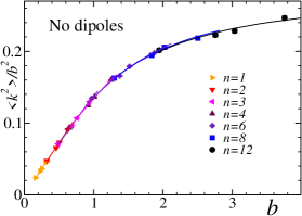
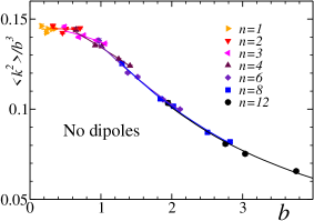
(a)	(b)

Figure 3: The density of the squared monopole charges, $\langle k^{2}_{s}\rangle$, with the UV dipoles removed. The density is normalized (a) by $b^{2}$ and (b) by $b^{3}$. The fits by the function (22) are shown by dashed lines for each value of the blocking step, $n$.

According to the prediction coming from the Coulomb gas model (29) the ratio $\langle k^{2}_{s}\rangle/b^{3}$ should tend to a constant as $b$ becomes smaller. This behavior can indeed be seen from Figure 3(b). Note that at small values of $b$ the $b$–scaling of the monopole density is violated. This scaling violation is not unexpected due to the presence of the lattice artifacts at the scale $b\sim a$. In order to get artifact–free results we will use below large–$b$ monopoles.

The values of the parameters of the Coulomb gas model in the continuum limit, Eq. (2), can be obtained by fitting the numerical results for $\langle k^{2}_{s}\rangle$ by the theoretical prediction (22),(17). Technically, for each value of the blocking step, $n$, we have a set of the data corresponding to different values of the lattice coupling $\beta$, and, consequently, to different values of $b=n\cdot a(\beta)$. Note that by fixing $n$ we simultaneously fix the extension of the coarse lattice, $L/n$, in units of $b$. The size of the coarse lattice enters in Eq. (17). We fit the set of the data for the fixed blocking step $n$. The best fit curves are shown in Figures 3(a) and (b) by dashed lines. The quality of the fit is very good, $\chi^{2}/d.o.f.\sim 1$.

The fits of the density provide us with the values of the continuum monopole density, $\rho^{(n)}$, and the Debye mass, $M^{(n)}_{D}$, obtained for the fixed blocking $n$. These results are shown (in units of the string tension) in Figures 4(a) and (b), respectively.

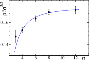
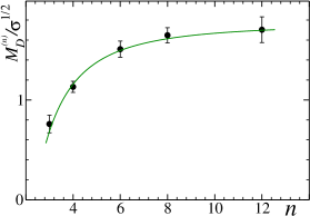
(a)	(b)

Figure 4: (a) The density of the continuum monopoles, $\rho$, and (b) the Debye screening mass, $M_{D}$, obtained with the help of the fits of the $n$–blocked squared monopole density by function (22). The large–$n$ extrapolation (66) is shown by solid lines.

We expect to get the artifact–free results in the limit of large $b$, or, in our case, in the limit of large $n$. Thus, one may naturally expect that in the limit $n\to\infty$ the values of $\rho^{(n)}$ and $M_{D}^{(n)}$ converge to the physical values: $\lim_{n\to\infty}{\cal O}^{(n)}={\cal O}^{\mathrm{ph}}$, where ${\cal O}$ stands for either $\rho$ or $M^{D}$. We found that the dependence of both $\rho$ and $M_{D}$ on the blocking size $n$ can be approximated by the dependence

$${\cal O}^{(n)}={\cal O}^{\mathrm{ph}}+{\mathrm{const}}\cdot n^{-2}\,,$$ (66)

at $n>2$ according to Figures 4(a,b). Using the extrapolation (66) we get the physical values for the monopole density $\rho$ and the Debye screening mass $M_{D}$ coming from the Coulomb gas model (here and below we omit the superscript ”ph” for the extrapolated values):

$$\rho\,/\sigma^{3/2}=0.174(2)\,,\qquad M_{D}\,/\sigma^{1/2}=1.77(4)\,.$$ (67)

The value of $M_{D}$ may be treated as the ”monopole contribution to the Debye screening mass”.

In order to check whether the monopole dynamics can be described by the Coulomb gas model (2) we construct the dimensionless quantity ref:3D

$$C=\frac{M_{D}\,\sigma}{\rho}\,,$$ (68)

which is known to be equal to eight ($C^{\mathrm{CG}}=8$) in the low density limit of the Coulomb gas model Polyakov . In Figure 5 we plot our numerical result for $C$ as a function of $n$.

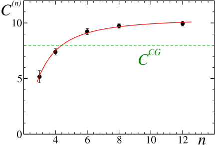
Figure 5: The same as in Figure 4 but for the ratio (68). The dashed line corresponds to the low density limit of Coulomb Gas model Polyakov , $C^{\mathrm{CG}}=8$.

Using the large–$n$ extrapolation (66) we get

$$C=10.1(1)\,,\qquad{\it i.e.}\qquad\frac{C}{C^{\mathrm{CG}}}=1.26(3)\,.$$ (69)

The quantity $C$ is about $25\%$ larger than that predicted by the Coulomb gas model in the low monopole density approximation, $C^{\mathrm{CG}}_{sp}=8$. The discrepancy is most likely explained by the invalidity of the assumption that the monopole density is low. Indeed, the low–density approach requires for the monopole density to be much lower than a natural scale for the density, $g^{6}$ (remember that the coupling $g$ has the dimensionality $mass^{1/2}$). The requirement $\rho\ll g^{6}$ can equivalently be reformulated as $\rho/M_{D}^{3}\gg 1$, which means that the number of the monopoles in a unit Debye volume, $Vol_{D}=\lambda_{D}^{3}\equiv M_{D}^{-3}$, must be high. Taking the numerical values for $\rho$ and $M_{D}$ from Eq. (67) we get: $\rho/M_{D}^{3}\approx 0.03\ll 1$. Thus, the low–density assumption is not valid in the 3D SU(2) gluodynamics. However, the discrepancy of $25\%$ observed in the quantity $C$, Eq. (69), is a good signal that the Coulomb gas model may still provide us with the predictions valid up to the specified accuracy.

One can compare our result for the monopole density, Eq. (67), with the result obtained by Bornyakov and Grigorev in Ref. Bornyakov , $\rho^{\mathrm{BG}}=2^{-7}(1\pm 0.02)\,g^{6}$. Using the result of Ref. Teper:StringTensions , $\sqrt{\sigma}=0.3353(18)\,g^{2}$, we get the value $\rho^{\mathrm{BG}}/\sigma^{3/2}=0.207(5)$, which is close to our independent estimation in the continuum limit (67): $\rho/\rho^{\mathrm{BG}}=0.83(4)$. The result of Ref. Bornyakov is about $20\%$ higher than our estimation for the monopole density. Thus, although the condition of the low monopole density approximation is strongly violated, the BFC method (based on the dilute gas approximation) gives the value of the monopole density which is consistent with other measurements.

It is interesting to compare the result for the screening mass (67) with the lightest glueball mass measured in Refs. Teper:StringTensions ; Teper:Glueball , $M_{O^{++}}=4.72(4)\,\sqrt{\sigma}$. In the Abelian picture, the mass of the ground state glueball obtained with the help of the correlator,

$$\langle F^{2}_{\mu\nu}(0)\,F^{2}_{\alpha\beta}(R)\rangle={\mathrm{const.}}\,e^{-M_{O^{++}}\,R}+\dots\,,$$

must be twice bigger than the Debye screening mass, $2M_{D}/M_{O^{++}}=1$, where the Debye mass is given by the following correlator

$$\langle F_{\mu\nu}(0)\,F_{\mu\nu}(R)\rangle={\mathrm{const.}}\,e^{-M_{D}\,R}+\dots\,.$$

The comparison of our result (67) with the result of Refs. Teper:StringTensions ; Teper:Glueball gives $2M_{D}/M_{O^{++}}=0.75(4)$. The deviation is of the order of $25\%$ similarly to case of the quantity $C$.

Finally, let us compare our result for the monopole contribution to the Debye screening mass, in Eq. (67), with the direct measurement of the Debye mass in 3D SU(2) gauge model made in Ref. Karsch , $m^{SU(2)}_{D}/\sqrt{\sigma}=1.39(9)$. The values agree with each other within the $25$ per cent: $m_{D}/m^{SU(2)}_{D}=1.27(11)$. Approximately the same accuracy is observed in the four–dimensional SU(2) gauge theory for the monopole contribution to the fundamental string tension ref:Bali .

IV.3 Short summary

The results of this Section indicate that the dynamics of the Abelian monopoles in the three–dimensional SU(2) gauge model can be described by the Coulomb gas model. Using a novel method called as the blocking of the monopoles from the continuum, we have calculated the monopole density and the Debye screening mass in the continuum using the numerical results for the (squared) monopole charge density. We have concluded that the Abelian monopole gas in the 3D SU(2) gluodynamics is not dilute. The self–consistency check of our results shows that the predictions of the Coulomb gas model for the monopole density and the Debye screening mass are consistent with the known data within the accuracy of $25\%$.

V Static monopoles in high temperature 4D gluodynamics

V.1 Details of simulations

Finite temperature system possesses a periodic boundary condition for time direction and the physical length in the time direction is limited to less than $1/T$. In this case it is useful to introduce anisotropic lattices. In the space direction, we perform the blockspin transformation and the continuum limit is taken as $a_{s}\to 0$ and $n_{s}\to\infty$ for a fixed physical scale $b=n_{s}a_{s}$. Here $a_{s}$ is the lattice spacing in the space directions and $n_{s}$ is the blockspin factor. In the time direction, the continuum limit is taken as $a_{t}\to 0$ and $N_{t}\to\infty$ for a fixed temperature $T=1/(N_{t}a_{t})$. Here $a_{t}$ is the lattice spacing in the time direction and $N_{t}$ is the number of lattice sites for the time direction. In general $a_{t}\neq a_{s}$ (anisotropic lattice). After taking the continuum limit, we finally get the effective monopole action which depends on the physical scale $b$ and the temperature $T$.

The anisotropic Wilson action for pure four-dimensional $SU(2)$ QCD is written as

$$S=\beta\Bigl{\{}\frac{1}{\gamma}\sum_{s,i>j\neq 4}P_{ij}(s)+\gamma\sum_{s,i\neq 4}P_{i4}(s)\Bigr{\}},$$ (70)

$$P_{\mu\nu}(s)\equiv\frac{1}{4}Tr\bigl{[}{\mathchoice{\rm 1\mskip-4.0mul}{\rm 1\mskip-4.0mul}{\rm 1\mskip-4.5mul}{\rm 1\mskip-5.0mul}}-U_{\mu}(s)U_{\nu}(s+\hat{\mu})U_{\mu}^{\dagger}(s+\hat{\nu})U_{\nu}^{\dagger}(s)\bigr{]}+h.c.$$ (71)

The procedure to determine the relation between the lattice spacings $a_{s}$, $a_{t}$ and the parameters $\beta$, $\gamma$ is described in Ref. NumericalMonopoleAction .

The monopole current is defined similarly to the three–dimensional case,

$$k_{\mu}(s)=\frac{1}{2}\epsilon_{\mu\nu\rho\sigma}\partial_{\nu}n_{\rho\sigma}(s+\hat{\mu})\,.$$ (72)

The monopole current satisfies the conservation law, $\partial_{\mu}^{\prime}k_{\mu}(s)=0$.

At a finite temperature the blockspin transformation of the spatial and temporal currents should be done separately NumericalMonopoleAction :

$$K_{\mu\neq 4}(s_{s},s_{4}) = \sum_{i,j=0}^{n_{s}-1}\sum_{l=0}^{n_{t}-1}k_{\mu\neq 4}\bigl{(}n_{s}s_{s}+(n_{s}-1)\hat{\mu}+i\hat{\nu}+j\hat{\rho},n_{t}s_{4}+l\bigr{)},$$ (73)

$$K_{4}(s_{s},s_{4}) = \sum_{i,j,l=0}^{n_{s}-1}k_{4}\bigl{(}n_{s}s_{s}+i\hat{\mu}+j\hat{\nu}+l\hat{\rho},n_{t}s_{4}+(n_{t}-1)\bigr{)},$$ (74)

where $n_{s}$ ($n_{t}$) is the number of blocking steps in space (time) direction.

We consider only the $n_{t}=1$ case since we are interested in high temperatures for which the monopoles are almost static. The lattice blocking is performed only in the spatial directions, $n_{s}=1\dots 8$, and we study only the static components $K_{4}$ among the $4D$ monopole currents $K_{\mu}$ (below we denote $K_{4}$ as $k$.). At high temperature we disregard the spatial currents $K_{i}$ since they are not interesting from the point of view of the long–range non–perturbative spatial physics. The size of the lattice monopoles is measured in terms of the zero temperature string tension, $\sigma_{T=0}$.

V.2 Monopole action

First, let us discuss the action for the static monopole currents. This action at high temperatures was found numerically in Ref. NumericalMonopoleAction using an inverse Monte–Carlo procedure. It turns out that the self–interaction of the temporal currents can be successfully described by the quadratic monopole action:

$$S_{mon}(k)=\sum_{i}f_{i}\,S_{i}(k)\,,$$ (75)

where $S_{i}$ are two–point operators of the monopole currents corresponding to different separations between the currents. The term $S_{1}$ corresponds to the zero distance between the monopoles, $S_{2}$ corresponds to the unit distance etc. (see Ref. NumericalMonopoleAction for further details). The two–point coupling constants $f_{i}$ of the monopole action are shown in Figures. 6(a,b) as a function of the distance between the lattice points. The numerical data corresponds to lowest, $T=1.6T_{c}$, and highest available temperatures, $T=4.8T_{c}$. The spatial spacings of the fine lattice, $a_{s}$, range from $a_{s}=.16\sigma^{-1/2}$ to $a_{s}=.25\sigma^{-1/2}$.

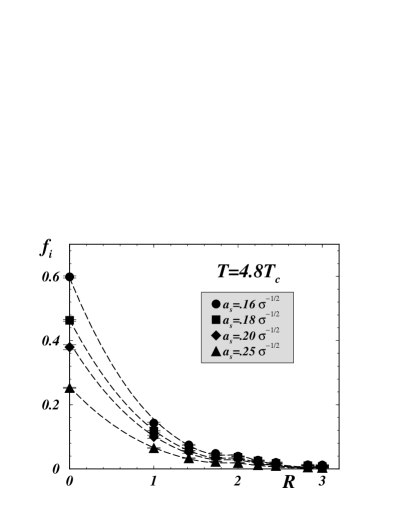
(a)		(b)

Figure 6: Two–point coupling constants, $f_{i}$, of the monopole action $vs.$ the distance between the lattice points, $r$ (in lattice units) for $n_{s}=6$, various spatial spacings, $a_{s}$, of the fine lattice. The temperature is (a) $T=1.6T_{c}$ and (b) $T=4.8T_{c}$. The fits by the Coulomb interaction (76) are visualized by the dashed lines.

According to Eq.(20) the leading term in the monopole action for large lattice monopoles ($b\gg\lambda_{D}$) must be proportional to the Coulomb interaction,

$$S_{mon}(k)=C_{C}\cdot\sum\limits_{s,s^{\prime}}k_{s}\,D_{s,s^{\prime}}\,k_{s^{\prime}}\,.$$ (76)

To check this prediction we fit the coupling constants $f_{i}$ by the Coulomb interaction (76) treating $C_{C}$ as a fitting parameter. The fits are visualized by the dashed lines in Figures 6(a,b). As one can see from the figures, this one-parametric fit works almost perfectly.

By fitting the action, we obtain the values of $C_{C}$ for a range of the lattice monopole sizes, $b\sqrt{\sigma}=.96\dots 1.5$ and the temperatures, $T=(1.6\dots 4.8)T_{c}$. According to Eq.(20) the pre–Coulomb coefficient $C_{C}(b,T)$ at sufficiently large monopole size $b\gg\lambda_{D}$ must depend on the lattice monopole size $b$ as follows:

$$C_{C}(b,T)=\frac{1}{R(T)\,b^{2}}\,,$$ (77)

where $R$ is the product of the screening length and the monopole density

$$R(T)=\lambda_{D}(T)\,\rho(T)\,.$$ (78)

We present the data for the pre-Coulomb coefficient, $C_{C}(b,T)$ and the corresponding one-parameter fits (77) in Figure 7(a). The fit is one–parametric with $R$ being the fitting parameter. Again we observe that the agreement between the data for $C_{C}$ and the fits is very good. We show the quantity $R$ $vs.$ temperature in Figure 7(b).

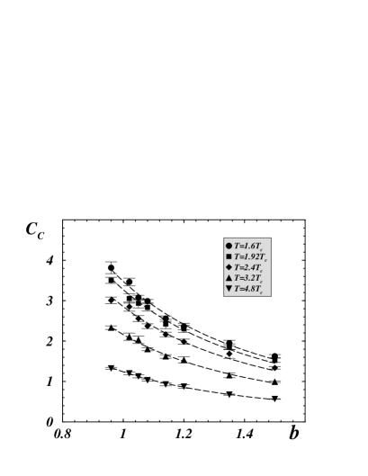
(a)		(b)

Figure 7: (a) The pre-Coulomb coupling $C_{C}$ and the fits of $C_{C}$ by Eq. (77) for various temperatures, $T$. (b) The product of the screening length and the monopole density, Eq.(78), calculated from the monopole action (in units of the string tension).

V.3 Monopole density

An independent information about the monopole dynamics can be obtained from the behavior of the lattice monopole density at various lattice monopole sizes. According to Eq.(29) the large-$b$ asymptotics of the quantity $\langle k^{2}(b)\rangle/b^{2}$ can be used to extract the product of the screening length and the continuum monopole density $R$, Eq.(78). We plot in Figures 8(a,b) the quantity $\langle k^{2}(b)\rangle/b^{2}$ $vs.$ the lattice monopole size $b$ for lowest and highest available temperatures.

(a)		(b)

Figure 8: The ratio $\langle k^{2}(b)\rangle/b^{2}$ $vs.$ lattice monopole size, $b$, at (a) $T=1.6\,T_{c}$ and (b) $T=4.8\,T_{c}$.

Our theoretical expectations (29) indicate that the function $\langle k^{2}(b)\rangle/b^{2}$ must vanish at small monopole sizes and tend to constant at large $b$. This behavior can be observed in our numerical data, Figure 8. The large-$b$ asymptotics of $\langle k^{2}(b)\rangle/b^{2}$ allows us to get the quantity ref:4Dhigh $R$ in Eq. (78).

V.4 Check of Coulomb gas picture

Let us denote $R_{act}$ ($R_{\rho}$) the quantity $R$ obtained from the behavior of the monopole action (density). From a numerical point of view these quantities are independent. Theoretically we expect that these quantities are equal. To check the self–consistency of our approach we plot the ratio of these quantities in Figure 9(a). It is clearly seen that the ratio is independent of the temperature and very close (with 10%–15% deviations) to unity, as expected.

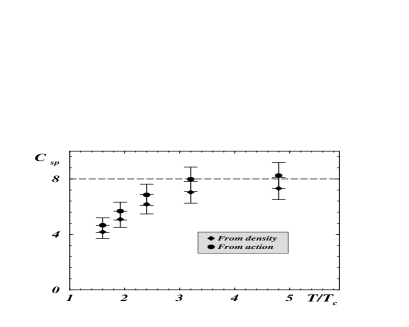
(a)		(b)

Figure 9: (a) Check of self–consistency: the ratio of the quantities $R$, Eq.(78) obtained from the lattice monopole action and density; (b) Check of the dilute Coulomb gas picture: quantities $C_{sp}$, Eq.(79), calculated from the action and density.

A check of the validity of the Coulomb gas picture can be obtained with the help of the quantity

$$C_{sp}(T)=\frac{\sigma_{sp}(T)}{\lambda_{D}(T)\,\rho(T)}\equiv\frac{\sigma_{sp}(T)}{R(T)}\,,$$ (79)

where $\sigma_{sp}$ is the spatial string tension. This quantity is similar to the one discussed in Eq. (68) in the previous Section. In the Abelian projection approach the spatial string tension should be saturated by the contributions from the static monopoles. In the dilute Coulomb gas of monopoles the string tension is Polyakov : $\sigma=8\sqrt{\rho}/g_{M}$ while the screening length is given by (3). These relations imply that in the dilute Coulomb gas of monopoles we should get $C_{sp}=8$.

We use the results for the spatial string tension of Ref. SigmaSP in the high temperature $SU(2)$ gluodynamics. It was found that for the temperatures higher than $T\approx 2T_{c}$ the spatial string tension can be well described by the formula: $\sigma_{sp}(T)=0.136(11)\cdot g^{4}_{4D}(T)\cdot T^{2}$, where $g_{4D}(T)$ is the four–dimensional $SU(2)$ 2–loop running coupling constant,

$$g^{-2}_{4D}(T)=\frac{11}{12\,\pi^{2}}\log\Bigl{(}\frac{T}{\Lambda_{T}}\Bigr{)}+\frac{17}{44\,\pi^{2}}\log\Bigl{[}2\log\Bigl{(}\frac{T}{\Lambda_{T}}\Bigr{)}\Bigr{]}\,,$$

with the scale parameter $\Lambda_{T}=0.076(13)\,T_{c}$. Taking also into account the relation between the critical temperature and the zero–temperature string tension Heller , $T_{c}=0.69(2)\,\sqrt{\sigma}$ we calculate the quantity $C_{sp}$ and plot it in Figure 9(b) as a function of the temperature, $T$. If the Coulomb picture works then $C_{sp}$ should be close to $8$. From Figure 9(b) we conclude that this is indeed the case at sufficiently high temperatures, $T/T_{c}\gtrsim 2.5$.

V.5 Short summary

The main result of this Section is that temporal currents of the Abelian monopoles in the SU(2) gluodynamics at high temperatures can be described by the three dimensional Coulomb model with a good accuracy. This result indicates that the non–zero value of the three dimensional (spatial) string tension at high temperatures is due to the temporal Abelian monopoles.

VI Monopole condensate in 4D gluodynamics

Finally, let us consider the SU(2) gluodynamics at zero temperature. The value of the monopole condensate $\eta$ was previously estimated from the chromoelectric string analysis of Ref. string:profile to be $\eta=194(19)$ MeV. Below we determine the value of the monopole condensate from the effective monopole action. We skip a description of the numerical simulations since it is quite similar to the one discussed in previous Sections (we use the isotropic Wilson action for the gauge fields and fix the Maximal Abelian gauge). We mention only the explicit construction of the extended $n^{3}$ monopoles

$$k_{\mu}^{(n)}(s)=\sum_{i,j,l=0}^{n-1}k_{\mu}(ns+(n-1)\hat{\mu}+i\hat{\nu}+j\hat{\rho}+l\hat{\sigma})\,.$$ (80)

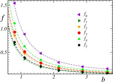
Figure 10: The fits of the $n=6$ monopole couplings by function (56).

We get the quadratic monopole action using the inverse Monte-Carlo simulations. The definition of the couplings $f_{i}$ of the monopole action is quite similar to the three–dimensional case discussed in previous Sections. The couplings are described in detail in Ref. ref:4D . We illustrate the success of the method showing the fitting of the couplings by the theoretical prediction (56) in Figure 10. The best fit parameters obtained from the fits of different couplings $f_{i}$ are very close to each other. This fact provides a nice self–consistency test of our approach. The numerical value of the monopole condensate turns out to be $\eta=243(42)$ MeV. This value is very close to the value $\eta=194(19)$ MeV obtained in Ref. string:profile using a completely different method.

VII Conclusions

The BFC method together with numerical simulations turns out to be a useful tool to obtain non–perturbative information about the topological defects in the continuum limit. The application of this method to the Abelian monopoles in SU(2) gauge model gives rise to the following results:

1. In the three dimensional SU(2) gluodynamics the Abelian monopoles can be described by the Coulomb gas model. The monopoles do not seem to be in the dilute gas regime. Nevertheless, the continuum values of the monopole density ($\rho=0.174(2)\,\sigma^{3/2}$) and the Debye screening mass ($M_{D}=1.77(4)\,\sigma^{1/2}$) – obtained with the help of the dilute monopole gas model – are consistent within the accuracy of $25\%$ with the known data obtained from independent measurements.

2. In the four dimensional SU(2) gluodynamics the static Abelian monopoles can also be described by the Coulomb gas model at high enough temperatures, $T\gtrsim 2.5\,T_{c}$. The monopoles form the dilute gas. The spatial string tension – obtained in independent measurements – is consistent with the prediction of the monopole Coulomb gas model. In other words, in the continuum the spatial string tension is dominated by contributions from the static monopoles.

3. In the four dimensional zero–temperature SU(2) gluodynamics the value of the monopole condensate, $\eta=243(42)$ MeV, was obtained in the framework of the dual superconductor picture. This result is consistent with the result obtained previously by an independent analysis.