Transport Coefficients of Gluon Plasma

Abstract

Transport coefficients of gluon plasma are calculated for a SU(3) pure gauge model by lattice QCD simulations on $16^{3}\times 8$ and $24^{3}\times 8$ lattices. Simulations are carried out at a slightly above the deconfinement transition temperature $T_{c}$, where a new state of matter is currently being pursued in RHIC experiments. Our results show that the ratio of the shear viscosity to the entropy is less than one and the bulk viscosity is consistent with zero in the region, $1.4\leq T/T_{c}\leq 1.8$.

Introduction: RHIC experiments have been bringing us many surprises. One of them is that the data are unexpectedly well described by the hydrodynamical model Star01 . Experimental data and phenomenological analyses suggest the quark-gluon plasma (QGP), or a new state of matter may be produced. See Ref.Ludlam for a review of RHIC experiments. Molnar and Gyulassy investigated the elliptic flow data using a Boltzmann-type equation for gluon scattering, and found that they needed a cross section about 50 times larger than expected in the perturbative QCDMolnar02 . This indicates that the QGP state above the phase transition temperature, $T_{c}$, is not a free gas of perturbed gluons. QCD-TARO collaboration measured the temporal meson propagators and found that their wave functions do not behave as free particles even at $T\sim 1.5T_{c}$; they conjectured that the strong interactions between the thermal gluons and quarks may provide binding forces. Recently, more extended analyses of the temporal propagators were reported by three groups Hatsuda03 ; Datta03 ; Umeda02 and it was suggested that the charmonium state survives until around $2T_{c}$.

The new state of matter produced at high temperatures in RHIC experiments is most likely not a weakly interacting plasma, but a strongly interacting quark-gluon system. Investigating the results in Ref.Molnar02 , Teaney found that $\eta/s\sim 0.04$, where $\eta$ and $s$ are the shear viscosity and the entropy, respectivelyTeaney03 . Shuryak and Zahed have proposed a ‘strongly coupled QGP’ model for the new state of matter above $T_{c}$ShuryakZahed , and argued that the QGP studied in RHIC is the most perfect fluid ever measured. Policastro et al. have calculated $\eta$ for the finite-temperature ${\cal N}=4$ supersymmetric Yang-Mills theory in the large $N$, strong-coupling regime, and obtained $\eta/s=1/4\pi$PTS01 . This value is found to be universal for theories with gravity duals and it is conjectured that $\eta/s=1/4\pi$ is a lower limit for all systems in natureKSS04 .

It has now become highly desirable to study the nature of the quark gluon system, particulaly its hydrodynamical parameters such as the transport coefficients above $T_{c}$ based on QCD in a non-perturbative manner. In this paper, we calculate the transport coefficients of QGP at a slightly above $T_{c}$, from the lattice simulations. Simulations are carried out in the quench approximation. For the calculation of the transport coefficients on a lattice, we apply the formulation based on the linear response theoryHorsley ; Zubarev ; Hosoya , where the transport coefficients are calculated from Matsubara Green’s function of energy momentum tensors. Numerical simulations of transport coefficients with this formulation were first carried out by Karsch and WyldKarsch . In their pioneering work, they performed the simulation on an $8^{3}\times 4$ lattice but unfortunately, the size in the imaginary time direction was too small for the determination of the transport coefficients.

We report here our simulation on a $N_{T}=8$ lattice with RG (renormalization group) improved action by Iwasaki. Our results are summarized as follows.

1. The ratio of the shear viscosity to the entropy, $\eta/s$, is small, i.e., less than one, but it is most probably larger than $1/4\pi$. See Fig.2.

2. The bulk viscosity is less than the shear viscosity and is consistent with zero within the present statistics.

3. For the heat conductivity, we could obtain no meaningful result. This is because, in pure gauge theory, there is no conserved current which transports the heat.

Preliminary results based on $16^{3}\times 8$ and smaller lattices have been reported at lattice and Quark Matter conferencesQM97 ; sakaist .

Transport Coefficients in Linear Response Theory: The formulation for the transport coefficients of QGP in the framework of the linear response theory has been given in Refs.Horsley ; Zubarev ; Hosoya . For the sake of consistency, we shall summarize the formula which will be used in the following calculations.

Transport coefficients are calculated using the space-time integral of a retarded Green’s function of energy momentum tensors,

$$\eta=-\int<T_{12}(\vec{x},t)T_{12}(\vec{x}^{\prime},t^{\prime})>_{ret},$$ (1)

$$\frac{4}{3}\eta+\zeta=-\int<T_{11}(\vec{x},t)T_{11}(\vec{x}^{\prime},t^{\prime})>_{ret},$$ (2)

$$\chi=-\frac{1}{T}\int<T_{01}(\vec{x},t)T_{01}(\vec{x}^{\prime},t^{\prime})>_{ret},$$ (3)

where $\int\equiv\int d^{3}x^{\prime}\int_{-\infty}^{t}dt_{1}e^{\epsilon(t_{1}-t)}\int_{-\infty}^{t_{1}}dt^{\prime}$, and $\eta$, $\zeta$ and $\chi$ represent shear viscosity, bulk viscosity and heat conductivity, respectively. $<T_{\mu\nu}T_{\rho\sigma}>_{ret}$ is the retarded Green’s function of the energy momentum tensors at finite temperature. For the pure gauge theory, $T_{\mu\nu}$’s are written by the field strength tensors $F_{\mu\nu}$:

$$T_{\mu\nu}=2\,\mbox{Tr}\,[F_{\mu\sigma}F_{\nu\sigma}-\frac{1}{4}\delta_{\mu\nu}F_{\rho\sigma}F_{\rho\sigma}].$$ (4)

$F_{\mu\nu}$ are defined by plaquette variables on the lattice as $U_{\mu\nu}(x)=\exp{(ia^{2}gF_{\mu\nu}(x))}$. $F_{\mu\nu}$ are obtained either by taking the $log$ of $U_{\mu\nu}$ directly, or by expanding $U_{\mu\nu}$ with respect to $a^{2}g$. In the following, we use the latter method to calculate $F_{\mu\nu}$Karsch .

It is difficult to calculate the retarded Green’s functions in the lattice QCD, in which Matsubara Green’s functions are measured. The retarded Green’s functions are obtained by the analytic continuation. We obtain the numerical values of Matsubara Green’s functions at discrete variables $\omega_{n}=2\pi nT$ in the momentum space, while the retarded Green’s functions are functions of the continuous variable $p_{0}$. Therefore, we need a bridge for the analytic continuation.

Matsubara Green’s functions $G_{\beta}$ are expressed in a Fourier transformed form with the spectral function $\rho$:

$$G_{\beta}(\vec{p},t)=\sum_{n}e^{i\omega_{n}t}\int d\omega\frac{\rho(\vec{p},\omega)}{i\omega_{n}-\omega}.$$ (5)

It is well known that the spectral function is common to both the retarded and Matsubara Green’s functionsHNS93 . The expression for the retarded Green’s functions is obtained by putting $\omega\rightarrow p_{0}+i\epsilon$.

The determination of $\rho(\vec{p},\omega)$ is not straightforward, because in a numerical simulation, Matsubara Green’s function has a finite number of points in the temperature direction, $N_{T}/2$. We must employ an ansatz for the spectral function with parameters, which are determined by fitting Matsubara Green’s function. The simplest nontrivial ansatz for the spectral function has been proposed by Karsch and WyldKarsch ,

$$\rho(\vec{p}=0,\omega)=\frac{A}{\pi}(\frac{\gamma}{(m-\omega)^{2}+\gamma^{2}}-\frac{\gamma}{(m+\omega)^{2}+\gamma^{2}}),$$ (6)

where $\gamma$ represents the effects of interactions and is related to the imaginary part of the selfenergy. This ansatz is supported by perturbative calculationsHorsley ; Hosoya .

Once we use this ansatz for the spectral function, the space time integral of the retarded Green’s function can be calculated analytically. The result is

$$\alpha=2A\frac{2\gamma m}{(\gamma^{2}+m^{2})^{2}},$$ (7)

where $\alpha$ represents the shear viscosity $\eta$, bulk viscosity $\zeta$ or heat conductivity $\chi$ times $T$. At least three independent data points for Matsubara Green’s functions are necessary to determine these parameters.

In Ref.Karsch , a simulation was carried out on a $8^{3}\times 4$ lattice, where two independent data points in the temperature direction are available. In this simulation, three parameters in the spectral function could not be determined. In order to determine $A$, $\gamma$ and $m$, we adopt $N_{T}=8$.

Numerical Simulations: We calculate the transport coefficients in the $SU(3)$ gauge theory for the regions a slightly above the transition temperature which are covered in RHIC experiments. We adopt Iwasaki’s improved gauge action, which is closer to the renormalized trajectory than the plaquette action, and we obtain results close to the continuum limit on relatively coarse latticesYoshie . We found that the fluctuation of the Matsubara Green’s function is much suppressed comparing with the standard plaquette actionsakaied .

We should first determine the critical $\beta$ of Iwasaki’s improved action on the $N_{T}=8$ lattice. For the $N_{T}=4$ and $6$ lattices, the critical $\beta$ for this action were determined by the Tsukuba groupKaneko . We have carried out a simulation for $\beta_{c}$ on a $16^{3}\times 8$ lattice; the results were reported in Ref.sakaied . However, the volume size was small, and we could obtain only a rough estimation of $\beta_{c}$, that is, $2.70<\beta_{c}<2.72$. If we use the finite size scaling formula reported by the Tsukuba group, $\beta_{c}$ at $N_{T}=8$ becomes $2.72<\beta_{c}<2.74$. The values of $\beta_{c}$ determined by the simulation for $N_{T}=4,6,8$ do not yet satisfy the asymptotic two-loop scaling relation. We take $\beta=3.05$, $3.2$ and $3.3$ as our simulation points.

Matsubara Green’s Function on $N_{T}=8$ Lattice: The parameters of the simulations and the obtained statistics are summarized in Table 1. For Matsubara Green’s functions $G_{11}$ and $G_{12}$ from which the shear and bulk viscosities are calculated, we can obtain reliable signals from approximately $0.8\times 10^{6}$ MC data on a $24^{3}\times 8$ lattice. As an example, $G_{12}$ is shown in Fig.1 for $\beta=3.3$.

	$\beta$	total sweeps	For equilibrium	bin size
	3.05	1333900	133900	100000
$16^{3}$	3.2	1212400	112100	100000
	3.3	1265500	165500	100000
$24^{3}$	3.05	861000	61000	100000
	3.3	784000	84000	100000

Table 1: Simulation parameters and statistics. Data at $t=0$ and $t=8$ are not used for the fit.

In the case of the $16^{3}\times 8$ lattice, the errors are larger than the signal at $\tau=4$, even with more than $10^{6}$ Monte Carlo (MC) data. The volume of $16^{3}$ may be too small for $N_{T}=8$.

$G_{14}$, from which the heat conductivity is calculated, has too large a background noise to extract a signal. Therefore, the fitting of Matsubara Green’s function by the spectral function of Eq.(6) is carried out only for $G_{11}$ and $G_{12}$.

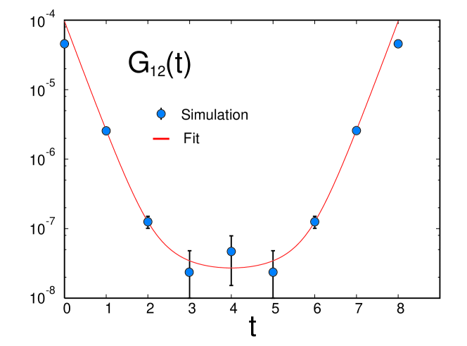
Figure 1: Numerical data points and fitting results of Matsubara Green’s function $G_{12}(t)$ on a $24^{3}\times 8$ lattice

Transport Coefficients of Gluon Plasma: The fitting of Matsubara Green’s function by Eq.(6) was carried out by applying a non-linear least-square fitting program, SALS. Then the transport coefficients of the gluon plasma are calculated using Eq.(7). The errors are estimated by the jackknife method. After equilibrium is reached, the data are grouped into bins and the average of the data in each bin is treated as an independent data sample. The bin size is changed from $5\times 10^{4}$ to $1.2\times 10^{5}$. The results are independent of the bin size. In the following, the bin size is $100000$ as shown in Table 1.

	$\beta$	$\eta a^{3}$	$\zeta a^{3}$	$\eta$ $\mbox{GeV}^{3}$	$\zeta$ $\mbox{GeV}^{3}$
	3.05	0.0018(28)	-0.0015(29)	0.054(82)	-0.044(85)
$16^{3}$	3.2	0.0059(46)	-0.0025(20)	0.281(223)	-0.122(90)
	3.3	0.0043(90)	-0.0041(142)	0.283(590)	-0.027(931)
$24^{3}$	3.05	0.0036(36)	-0.00095(288)	0.106(108)	-0.028(85)
	3.3	0.0072(30)	-0.0031(26)	0.471(194)	-0.201(167)

Table 2: Shear and bulk viscosities in non-dimension and in the physical units. The lattice scales, $a^{-1}=$ 3.09, 3.62 and 4.03 GeV for $\beta=$ 3.05, 3.20 and 3.30, respectively.

The results for the shear and bulk viscosities are given Table 2. The bulk viscosity is equal to zero within error bars, while the shear viscosity remains finite. We do not see the size dependence.

In the lattice calculations, the shear viscosity is calculated in the form $\eta\times a^{3}$. In order to express it in physical units, we should know the lattice spacing $a$ at each $\beta$ value. For the estimation of $a$, we use the finite temperature transition point $\beta_{c}$. We take $\beta_{c}=2.73$ for $N_{T}=8$. The transition temperature is $T_{c}=276MeV$Kaneko , and assume asymptotic two-loop scaling for the region $\beta>2.73$. The lattice spacing and the shear and bulk viscosities in the physical units are also listed in Table 2. $\eta^{1/3}$ expressed in the physical units are slightly less than the ordinary hadron masses around $T_{c}$.

Entropy density: In a homogeneous system, the free energy has the form of $F=fV$, and then the pressure is $p=-f$. Using the thermodynamical relation, $U-TS=-T\log Z=F$, we obtainBoyd96

$$s=S/V=(\epsilon+p)/T,$$ (8)

where $\epsilon$ is the energy density. Using lattices with $N_{T}=8$ and the integration method, $p/T^{4}|_{\beta_{0}}^{\beta}=\int_{\beta_{0}}^{\beta}d\beta^{\prime}N_{T}^{4}(\langle S\rangle_{T}-\langle S\rangle_{0})$, CP-PACS obtained $p$ and $\epsilon$, where $\langle S\rangle_{T}$ and $\langle S\rangle_{0}$ are the expectation values of the action density at temperature $T$CPPACS99 . We reconstruct the results from their numerical data of $\langle S\rangle_{T}$ and $\langle S\rangle_{0}$ and calculate the entropy density in Eq.(8).

Concluding Remarks: In the high temperature limit, the transport coefficients have been calculated analytically by the perturbation method Kajantie ; Horsley ; Gavin ; BMPR90 ; Arnold00 ; Arnold03 . They are summarized as follows.
(1) The bulk viscosity is smaller than the shear viscosity. This is consistent with our numerical results. (2) The shear viscosity in the next-to-leading-log is expressed by Arnold03 , $\eta_{NLL}=({T^{3}}/{g^{4}}){C_{1}}/{\log(\mu^{*}/m_{D})}$ where $m_{D}=\sqrt{1+N_{f}/6}gT$, and for the pure gluon system $C_{1}=27.126$ and $\mu^{*}/T=2.765$ .

There is a slight ambiguity in the relationship between coupling $g$ and the temperature, and we use a simple form, $g^{-2}=2b_{0}\log(4T/\Lambda)$ with $b_{0}=11N_{c}/48\pi^{2}$. The scale parameter $\Lambda$ on the lattice is set to be $\Lambda/T_{c}\simeq 1.5$. For the entropy density, we use a hard-thermal loop resultBlaizot99 . With these formulae, the perturbative $\eta/s$ can be compared with the results of numerical calculations. The result is shown in Fig.2.

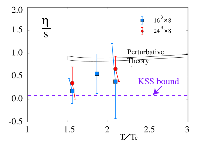
Figure 2: The ratio of the shear viscosity to the entropy as a function of $T/T_{c}$ KSS bound is $1/4\pi$KSS04 . ‘Perturbative theory’ is constructed from $\eta$ in Ref.Arnold03 and $s$ in Ref.Blaizot99 .

In this letter, we report the first lattice QCD result of the transport coefficients in the vicinity of the critical temperature. Although it still contains large errors, it may provide useful information for understanding QGP in these temperature regions. In particular, a small $\eta/s$ supports the success of the hydrodynamical description for QGP. Applicability conditions of the hydrodynamical model in quantum field theory were first considered in Ref.Namiki59 . Together with experimental and phenomenological studies, the field theoretical approach will enrich our understanding of the new state of matter. We have shown here that the lattice QCD numerical simulations can provide useful information.

The next step is to obtain data with smaller systematic and statistical errors. If we can reduce the error bars in Fig.2 by a factor of two or three, we may realistically compare the data with the conjecture in Ref.KSS04 . We observed that Matsubara Green’s function suffer from large fluctuations, but by using the improved action the fluctuations are significantly reduced. Another possibility for reducing the fluctuations may be to employ improved operators for $T_{\mu\nu}$Tsumura .

The results here depend on the ansatz of the spectral function of the Fourier transform of Matsubara Green’s function. In order to test the functional form of the spectral function, we need more data points for Matsubara Green’s function in the temperature direction, for which the most effective approach will be to apply an anisotropic lattice. If we have sufficient data points, the maximum entropy method is a promising way of determining the spectral functionMEM00 which is free from the ansatz. Aarts and Resco pointed out, however, that it is difficult to extract transport coefficients in weakly-coupled theories from the euclidean lattice, since Green’s function is insensitive to details of the spectral function $\rho(\omega)$ at small $\omega$Aarts02 . New concepts will be necessary to overcome this diffculty.

Acknowledgement We thank Tetsuo Hatsuda and Kei Iida for many useful discussions and their constant encouragement. One of the authors (A.N.) would like to thank Andrei Starinets for his kind and patient explanations of Refs.PTS01 and KSS04 for the author who is ignorant of this field. The simulations were carried out at KEK and at RCNP.

References

- (1) STAR Collaboration: K.H. Ackermann, et al., Phys. Rev. Lett. 86 (2001) 402. (nucl-ex/0009011).
- (2) T. Ludlam, Talk at “New Discoveries at RHIC – The Stongly Interactive QGP”, BNL, May 14-15, 2004, http://quark.phy.bnl.gov/ mclerran/qgp/
- (3) D. Molnar and M. Gyulassy, Nucl. Phys. A697 (2002) 495; Erratum in Nucl. Phys. A703 (2002) 893, (nucl-th/0104073); D. Molnar, hep-ph/0111401.
- (4) M. Asakawa and T. Hatsuda, Phys. Rev. Lett. 92 (2004) 012001, (hep-lat/0308034).
- (5) S. Datta, F. Karsch, P. Petreczky and I. Wetzorke Phys. Rev. D69 (2004) 094507, (hep-lat/0312037).
- (6) T. Umeda, K. Nomura and H. Matsufuru, hep-lat/0211003.
- (7) D. Teaney, nucl-th/0301099.
- (8) E. V.Shuryak and I. Zahed, hep-ph/0403127; E.V.Shuryak, hep-ph/0405066.
- (9) G. Policastro, D.T.Son and A.O.Starinets, Phys. Rev. Lett. 87 (2001) 081601,. (hep-th/0104066).
- (10) P. Kovtun, D.T.Son and A.O.Starinets, hep-th/0405231.
- (11) R.Horsley and W.Schoenmaker, Nucl. Phys. B280[FS18](1987),716, ibid.,735.
- (12) D.N.Zubarev, ‘Nonequilibrium Statistical Thermodynamics’, Plenum, New York 1974.
- (13) A.Hosoya, M.Sakagami and M Takao, Annals of Phys.154(1984) 229.
- (14) F.Karsch and H.W.Wyld, Phys. Rev. D35 (1987) 2518.
- (15) S. Sakai, A. Nakamura and T. Saito, Nucl. Phys. A638 (1998) 535, (hep-lat/9810031).
- (16) A. Nakamura, S. Sakai and K. Amemiya, Nucl. Phys.B(Proc Supple) 53 (1997), 432.
- (17) T.Hashimoto, A.Nakamura and I.O.Stamatescu, Nucl. Phys. B400, (1993) 267.
- (18) Y. Iwasaki et al., Nucl. Phys. B(PS) 42 (1995) 502, and references therin.
- (19) A. Nakamura, T.Saito and S. Sakai, Nucl. Phys.B(PS) 63 (1998) 424.
- (20) Y.Iwasaki et al., Nucl. Phys. B(PS) 53 (1997) 426.
- (21) G. Boyd et al., Nucl. Phys. B469 (1996) 419, (hep-lat/9602007).
- (22) M. Okamoto et al., Phys. Rev. D60 (1999) 094510. (hep-lat/9905005)
- (23) A.Hosoya and K. Kajantie, Nucl.Phys.B250(1985),666.
- (24) S. Gavin, Nuclear Phys. A345(1985) 826.
- (25) G. Baym, H. Monien, C. J. Pethick and D. G. Ravenhall, Phys. Rev. Lett. 16 (1990) 1867.
- (26) P. Arnold, G. D. Moore and L. G. Yaffe, JHEP 0011 (2000) 001, (hep-ph/0010177).
- (27) P. Arnold, G. D. Moore and L. G. Yaffe, JHEP 0305 (2003) 051, (hep-ph/0302165).
- (28) J.-P. Blaizot, E. Iancu, A. Rebhan, Phys.Rev.Lett. 83 (1999) 2906, (hep-ph/9906340).
- (29) C. Iso, K. Mori and M. Namiki, Prog. Theor. Phys. 22 (1959) 403.
- (30) M. Asakawa and K. Tsumura, work in progress.
- (31) M. Asakawa, T. Hatsuda and Y. Nakahara, Prog. Part. Nucl. Phys. 46 (2001) 459, (hep-lat/0011040).
- (32) G. Aarts and J. M. Martinez Resco, JHEP 0204 (2002) 053, (hep-ph/0203177).