On the discretization of physical momenta in lattice QCD

Abstract

The adoption of two distinct boundary conditions for two fermions species on a finite lattice allows to deal with arbitrary relative momentum between the two particle species, in spite of the momentum quantization rule due to a limited physical box size. We test the physical significance of this topological momentum by checking in the continuum limit the validity of the expected energy-momentum dispersion relations.

1 Introduction

Among the restrictions of field theory formulations on a lattice, the finite volume momentum quantization represents a severe limitation in various phenomenological applications. For example, in a two body hadron decay where the energies of the decay products, related by 4–momentum conservation to the masses of the particles involved, cannot assume their physical values unless these masses are consistent with the momentum quantization rule. In this letter we propose a solution to the problem based on the use of different boundary conditions for different fermion species.

We test the idea in the simplest case of a flavoured quark-antiquark correlation used to determine asymptotically the energy of the corresponding meson. In this case the fermion and the antifermion are the different fermion species and we show that suitable different boundary conditions can propagate a meson with a momentum that can assume continuous values.

Section 2 introduces the boundary conditions, section 3 reports on the numerical results and section 4 summarizes the conclusions.

2 Generalized boundary conditions

In order to explain the method to have continuous physical momenta on a finite volume we first re–derive, for the sake of clarity, the momentum quantization rule in the case of a particle with periodic boundary conditions (PBC). To this end we consider a fermionic field $\psi(x)$ on a 4–dimensional finite volume of topology $T\times L^{3}$ with PBC in the spatial directions

$$\psi(x+\vec{e}_{i}\ L)=\psi(x)\;,\qquad i=1,2,3$$ (1)

This condition can be re-expressed by Fourier transforming both members of the previous equation

$$\int{d^{4}p\ e^{-ip(x+\vec{e}_{i}\ L)}\ \tilde{\psi}(p)}=\int{d^{4}p\ e^{-ipx}\ \tilde{\psi}(p)}\;,\qquad i=1,2,3$$ (2)

It follows directly from the previous relation that, in the case of periodic boundary conditions, one has

$$e^{ip_{i}L}=1\quad\Longrightarrow\quad p_{i}=\frac{2\pi\ n_{i}}{L}\;,\quad i=1,2,3$$ (3)

where the $n_{i}$’s are integer numbers. The authors of [1] have first considered a generalized set of boundary conditions, that here we call $\theta$–boundary conditions ($\theta$–BC), depending upon the choice of a topological 3–vector $\vec{\theta}$

$$\psi(x+\vec{e}_{i}\ L)=e^{i\theta_{i}}\ \psi(x)\;,\qquad i=1,2,3$$ (4)

The modification of the boundary conditions affects the zero of the momentum quantization rule. Indeed, by re-expressing equation (4) in Fourier space, as already done in the case of PBC in equation (2), one has

$$e^{i(p_{i}-\frac{\theta_{i}}{L})L}=1\quad\Longrightarrow\quad p_{i}=\frac{\theta_{i}}{L}+\frac{2\pi\ n_{i}}{L}\;,\quad i=1,2,3$$ (5)

It comes out that the spatial momenta are still quantized as for PBC but shifted by an arbitrary continuous amount ($\theta_{i}/L$). The observation that this continuous shift in the allowed momenta it is physical and can be thus profitably used in phenomenological applications is the key point of the present work. The generalized $\theta$–dependent boundary conditions of equation (4) can be implemented by making a unitary Abelian transformation on the fields satisfying $\theta$–BC

$$\psi(x)\quad\longrightarrow\quad{\mathcal{U}}\ (\theta,x)\psi(x)=e^{-\frac{i\theta x}{L}}\ \psi(x)$$ (6)

As a consequence of this transformation the resulting field satisfies periodic boundary conditions but obeys a modified Dirac equation

$$S[\bar{\psi},\psi]\quad \longrightarrow \quad\sum_{x,y}{\bar{\psi}(x)\ {\mathcal{U}}(\theta,x)D(x,y){\mathcal{U}}^{-1}(\theta,y)\ \psi(y)}$$ (7)

$$= \quad\sum_{x,y}{\bar{\psi}(x)\ D_{\theta}(x,y)\ \psi(y)}$$

where the $\theta$–dependent lattice Dirac operator $D_{\theta}(x,y)$ is obtained by starting from the preferred discretization of the Dirac operator and by modifying the definition of the covariant lattice derivatives, i.e. by passing from the standard forward and backward derivatives:

$$\nabla_{\mu}\psi(x) = \frac{1}{a}\left[U_{\mu}(x)\psi(x+a\ \hat{\mu})-\psi(x)\right]$$

$$\nabla^{\dagger}_{\mu}\psi(x) = \frac{1}{a}\left[\psi(x)-U^{-1}_{\mu}(x-a\ \hat{\mu})\psi(x-a\ \hat{\mu})\right]$$ (8)

to the $\theta$–dependent ones

$$\nabla_{\mu}(\theta)\psi(x) = \frac{1}{a}\left[\lambda_{\mu}\ U_{\mu}(x)\psi(x+a\ \hat{\mu})-\psi(x)\right]$$

$$\nabla_{\mu}(\theta)^{\dagger}\psi(x) = \frac{1}{a}\left[\psi(x)-\lambda_{\mu}^{-1}\ U^{-1}_{\mu}(x-a\ \hat{\mu})\psi(x-a\ \hat{\mu})\right]$$ (9)

where we have introduced

$$\lambda_{\mu}=e^{\frac{ia\theta_{\mu}}{L}}\qquad\theta_{0}=0$$ (10)

The authors of ref. [2] have considered for the first time $\theta$–BC in perturbative phenomenological applications. They used the shift in the momentum quantization rule, that they called a “finite size momentum”, in order to build an external source to probe the tensor structure of the Wilson operators. A similar analysis was then repeated non–perturbatively by the same group in ref. [3]. The use of $\theta$–BC has been considered in different contexts also in [4, 5, 6, 7, 8].

In this work we point out that the term $\vec{\theta}/L$ acts as a true physical momentum.

As a test, we calculate the energy of a meson made up by two different quarks with different $\theta$–BC for the two flavours. We work in the $O(a)$–improved Wilson–Dirac lattice formulation of the QCD within the Schrödinger Functional formalism [9, 10] but, we want to stress that the use of $\theta$–BC in the spatial directions is completely decoupled from the choice of time boundary conditions and can be profitably used outside the Schrödinger Functional formalism, for example in the case of standard periodic time boundary conditions. Let us consider the following correlators

$$f_{P}^{ij}(\theta;x_{0})=-\frac{a^{6}}{2}\sum_{\vec{y},\vec{z},\vec{x}}{\langle\ \bar{\zeta}_{i}(\vec{y})\gamma_{5}\zeta_{j}(\vec{z})\ \bar{\psi}_{j}(x)\gamma_{5}\psi_{i}(x)\ \rangle}$$ (11)

where $i$ and $j$ are flavour indices, all the fields satisfy periodic boundary conditions and the two flavours obey different $\theta$–modified Dirac equations, as explained in equations (7), (8) and (9). In practice it is adequate to choose the flavour $i$ with $\theta=0$, i.e. with ordinary PBC, and the flavour $j$ with $\theta\neq 0$. After the Wick contractions the pseudoscalar correlator of equation (11) reads

$$f_{P}^{ij}(\theta;x_{0})=\frac{a^{6}}{2}\sum_{\vec{y},\vec{z},\vec{x}}\mathop{\rm Tr}{\langle\ \gamma_{5}\ S_{j}(\theta;\vec{z},x)\ \gamma_{5}\ S_{i}(0;x,\vec{y})\ \rangle}$$ (12)

where $S(\theta;x,y)$ and $S(0;x,y)$ are the inverse of the $\theta$–modified and of the standard Wilson–Dirac operators respectively. Note that the projection on the momentum $\vec{\theta}/L$ of one of the quark legs in equation (12) it is not realized by summing on the lattice points with an exponential factor but it is encoded in the $\theta$–dependence of the modified Wilson–Dirac operator and, consequently, of its inverse $S(\theta;x,y)$.

This correlation is expected to decay exponentially at large times as

$$f_{P}^{ij}(\theta;x_{0})\qquad\stackrel{{\scriptstyle x_{0}\gg 1}}{{\longrightarrow}}\qquad f_{ij}\ e^{-ax_{0}E_{ij}(\theta,a)}$$ (13)

where, a part from corrections proportional to the square of the lattice spacing, $E_{ij}$ is the physical energy of the mesonic state

$$E_{ij}(\theta,a)=\sqrt{M_{ij}^{2}+\left(\frac{\vec{\theta}}{L}\right)^{2}}+O(a^{2})$$ (14)

here $M_{ij}$ is the mass of the pseudoscalar meson made of a $i$ and a $j$ quark anti–quark pair. In the next section we will show the calculation of the meson energies for different flavours and for different choices of $\vec{\theta}$. We will show that after the continuum extrapolations we will find the expected relativistic dispersion relations

$$E_{ij}^{2}=M_{ij}^{2}+\left(\frac{\vec{\theta}}{L}\right)^{2}$$ (15)

3 Numerical tests

All the results of this section are obtained in the quenched approximation of the QCD. We have done simulations on a physical volume of topology $T\times L^{3}$ with $T=2L$ and linear extension $L=3.2\ r_{0}$, where $r_{0}$ is a phenomenological distance parameter related to the static quark anti–quark potential [11]. In order to extrapolate our numerical results to the continuum limit we have simulated the same physical volume using three different discretizations with number of points $(32\times 16^{3})$, $(48\times 24^{3})$ and $(64\times 32^{3})$ respectively. We have fixed the three values of the bare couplings corresponding to the different discretizations using the $r_{0}$ scale with the numerical results given in [12]. All the parameters of the simulations are given in table 1.

$\bf\beta$		$\bf L/a$		$\bf k$	$\bf r_{0}\ m^{RGI}$
				0.132054	0.645(7)
5.960		16		0.132609	0.520(6)
				0.133315	0.362(5)
				0.133725	0.269(4)
				0.134208	0.655(9)
6.211		24		0.134540	0.521(7)
				0.134954	0.354(6)
				0.135209	0.251(5)
				0.134517	0.676(15)
6.420		32		0.134764	0.540(12)
				0.135082	0.365(10)
				0.135269	0.262(9)
$\bf[\theta_{x},\theta_{y},\theta_{z}]$	=	$[0.0,\ 0.0,\ 0.0]$	$[1.0,\ 1.0,\ 1.0]$	$[2.0,\ 2.0,\ 2.0]$	$[3.0,\ 3.0,\ 3.0]$

Table 1: Parameters of the simulations. The values of the bare couplings has been chosen in order to fix the extension of the physical volume $L=3.2\ r_{0}$. For each value of the $k$ parameter we have simulated all the values of $\vec{\theta}$.

The values of the RGI quark masses reported in table 1 have been calculated starting from the PCAC relation

$$m^{PCAC}_{ii}=\frac{\tilde{\partial_{0}}f_{A}^{ii}(0;x_{0})+ac_{A}\partial_{0}^{\dagger}\partial_{0}f_{P}^{ii}(0;x_{0})}{2f_{P}^{ii}(0;x_{0})}$$ (16)

where $\partial_{\mu}$, $\partial^{\dagger}_{\mu}$ are the usual forward and backward lattice derivatives respectively while $\tilde{\partial}_{\mu}$ is defined as $(\partial_{\mu}+\partial_{\mu}^{\dagger})/2$. The time correlator $f_{P}^{ij}(0;x_{0})$ has already been defined in equation (11) while $f_{A}^{ij}(0;x_{0})$ is defined in the following relation

$$f_{A}^{ij}(\theta;x_{0})=-\frac{a^{6}}{2}\sum_{\vec{y},\vec{z},\vec{x}}{\langle\ \bar{\zeta}_{i}(\vec{y})\gamma_{5}\zeta_{j}(\vec{z})\ \bar{\psi}_{j}(x)\gamma_{0}\gamma_{5}\psi_{i}(x)\ \rangle}$$ (17)

The improvement coefficient $c_{A}$ has been computed non–perturbatively in [13]. The RGI quark masses are connected to the PCAC masses of equation (16) from the following relation

$$m_{ii}^{RGI}=Z_{M}(g_{0})\ \left[1+(b_{A}-b_{P})\ am_{i}\right]\ m^{PCAC}_{ii}(g_{0})$$ (18)

where the renormalization factor $Z_{M}(g_{0})$ has been computed non–perturbatively in [14]. Also the difference of the improvement coefficients $b_{A}$ and $b_{P}$ is known non–perturbatively from [15, 16]. In (18) the masses $m_{i}$ are the bare ones defined as

$$am_{i}=\frac{1}{2}\left[\frac{1}{k_{i}}-\frac{1}{k_{c}}\right]$$ (19)

For each value of the simulated quark masses reported in table 1 we have inverted the Wilson–Dirac operator for three non–zero values of $\vec{\theta}$. Setting the lattice scale by using the physical value $r_{0}=0.5$ fm, the expected values of the physical momenta associated with the choices of $\vec{\theta}$ given in table 1 are simply calculated according to the following relation

$$|\vec{p}|\;=\;\frac{|\vec{\theta}|}{L}\;\simeq\;0.125\ |\vec{\theta}|\;\mbox{GeV}\quad=\quad\left\{\begin{array}[]{l}0.000\\ 0.217\\ 0.433\\ 0.650\\ \end{array}\right.\;\mbox{GeV}\qquad L\ \simeq\ 1.6\;\mbox{fm}$$ (20)

These values have to be compared with the value of the lowest physical momentum allowed on this finite volume in the case of periodic boundary conditions, i.e. $|\vec{p}|\simeq 0.785$ GeV.

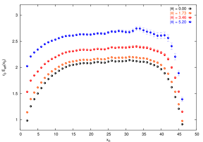
Figure 1: Effective energies $E_{eff}^{ij}(\theta,a;x_{0})$, as defined in eq. (21) at fixed cut–off. The results correspond to the simulation done at $\beta=6.211$ with $r_{0}\ m_{1}^{RGI}=0.655$ and $r_{0}\ m_{2}^{RGI}=0.354$. Similar figures could have been shown for other combinations of the simulated quark masses and for the other values of the bare coupling.

At fixed cut–off, for each combination of flavour indices and for each value of $\vec{\theta}$ reported in table 1 we have extracted the effective energy from the correlations of eq. (11), $f_{P}^{ij}(\theta;x_{0})$, as follows

$$a\ E_{eff}^{ij}(\theta,a;x_{0})\;=\;\frac{1}{2}\ \log\left(\frac{f_{P}^{ij}(\theta;x_{0}-1)}{f_{P}^{ij}(\theta;x_{0}+1)}\right)$$ (21)

In fig. 1 we show this quantity for the simulation performed at $\beta=6.211$ corresponding to $r_{0}\ m_{1}^{RGI}=0.655$ and $r_{0}\ m_{2}^{RGI}=0.354$, for each simulated value of $\vec{\theta}$. As can be seen the correlations with higher values of $|\vec{\theta}|$ are always greater than the corresponding ones with lower values of the physical momentum

$$|\vec{\theta}_{1}|>|\vec{\theta}_{2}|\quad\Rightarrow\quad E_{eff}^{ij}(\theta_{1},a;x_{0})>E_{eff}^{ij}(\theta_{2},a;x_{0})$$ (22)

a feature that will be confirmed in the continuum limit.

In the continuum extrapolations we have fixed the physical values of the quark masses slightly interpolating the simulated sets of numerical results.

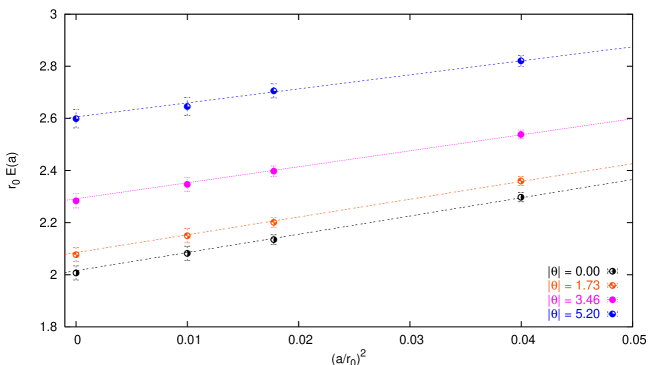
Figure 2: Continuum extrapolations of the plateau averaged effective energies $E^{ij}(\theta,a)$. The results correspond to the quark masses $r_{0}\ m_{1}^{RGI}=0.650$ and $r_{0}m_{2}^{RGI}=0.350$. Similar figures could have been shown for other combinations of the simulated quark masses.

Being interested in the ground state contribution to the correlation of eq. (11), we have averaged the effective energies over a ground state plateau of physical length depending upon the quark flavours. We call $E^{ij}(\theta,a)$ the result of the average and in fig. 2 we show a typical continuum extrapolation of this quantity. Similar figures could have been shown for the other values of simulated quark masses.

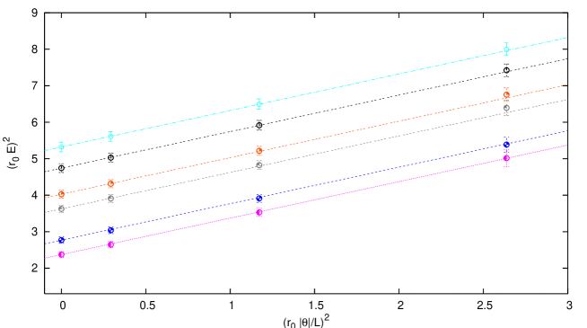
Figure 3: Continuum dispersion relations. The data correspond to different combinations of the simulated quark masses and reproduce very well the expected theoretical behavior, i.e. straight lines having as intercepts the meson masses and as angular coefficients one (see eq. 15).

The continuum results verify very well the dispersion relations of equation (15) as can be clearly seen from fig. 3 in which the square of $E^{ij}(\theta)$ for various combinations of the flavour indices is plotted versus the square of the physical momenta $|\vec{\theta}|/L$. The plotted lines have not been fitted but have been obtained by using as intercepts the simulated meson masses and by fixing their angular coefficients to one.

4 Conclusions

We have argued that the limitation represented by the finite volume momentum quantization rule can be overcame by using different boundary conditions for different fermion species.

We have supported this observation by calculating the relativistic dispersion relations satisfied by a set of pseudoscalr mesons in the case of quenched lattice QCD. We have shown that the physical momentum carried by these particles can be varied continuously by enforcing different $\theta$–boundary conditions (see eq. (4)) for the two quarks inside the mesons.

The method proposed can be applied to study all the quantities of phenomenological interest that would benefit from the introduction of continuous physical momenta like, for example, weak matrix elements. The suggestion can be applied in quenched QCD also in the case of flavourless mesons while can be extended to full QCD in the flavoured case only.

References

- [1] K. Jansen et al., Phys. Lett. B372 (1996) 275, hep-lat/9512009.
- [2] A. Bucarelli et al., Nucl. Phys. B552 (1999) 379, hep-lat/9808005.
- [3] Zeuthen-Rome / ZeRo, M. Guagnelli et al., Nucl. Phys. B664 (2003) 276, hep-lat/0303012.
- [4] P.F. Bedaque, (2004), nucl-th/0402051.
- [5] D.J. Gross and Y. Kitazawa, Nucl. Phys. B206 (1982) 440.
- [6] J. Kiskis, R. Narayanan and H. Neuberger, Phys. Rev. D66 (2002) 025019, hep-lat/0203005.
- [7] J. Kiskis, R. Narayanan and H. Neuberger, Phys. Lett. B574 (2003) 65, hep-lat/0308033.
- [8] A. Roberge and N. Weiss, Nucl. Phys. B275 (1986) 734.
- [9] M. Luscher et al., Nucl. Phys. B384 (1992) 168, hep-lat/9207009.
- [10] S. Sint, Nucl. Phys. B421 (1994) 135, hep-lat/9312079.
- [11] R. Sommer, Nucl. Phys. B411 (1994) 839, hep-lat/9310022.
- [12] S. Necco and R. Sommer, Nucl. Phys. B622 (2002) 328, hep-lat/0108008.
- [13] M. Luscher et al., Nucl. Phys. B491 (1997) 323, hep-lat/9609035.
- [14] ALPHA, S. Capitani et al., Nucl. Phys. B544 (1999) 669, hep-lat/9810063.
- [15] G.M. de Divitiis and R. Petronzio, Phys. Lett. B419 (1998) 311, hep-lat/9710071.
- [16] ALPHA, M. Guagnelli et al., Nucl. Phys. B595 (2001) 44, hep-lat/0009021.