Numerical Methods for the QCD Overlap Operator: III. Nested Iterations

Abstract

The numerical and computational aspects of chiral fermions in lattice quantum chromodynamics are extremely demanding. In the overlap framework, the computation of the fermion propagator leads to a nested iteration where the matrix vector multiplications in each step of an outer iteration have to be accomplished by an inner iteration; the latter approximates the product of the sign function of the hermitian Wilson fermion matrix with a vector.

In this paper we investigate aspects of this nested paradigm. We examine several Krylov subspace methods to be used as an outer iteration for both propagator computations and the Hybrid Monte-Carlo scheme. We establish criteria on the accuracy of the inner iteration which allow to preserve an a priori given precision for the overall computation. It will turn out that the accuracy of the sign function can be relaxed as the outer iteration proceeds. Furthermore, we consider preconditioning strategies, where the preconditioner is built upon an inaccurate approximation to the sign function. Relaxation combined with preconditioning allows for considerable savings in computational efforts up to a factor of 4 as our numerical experiments illustrate. We also discuss the possibility of projecting the squared overlap operator into one chiral sector.

, , , , and

1 Introduction

For two decades numerical simulations of very light quarks within lattice quantum chromodynamics have remained intractable as the chiral symmetry of the underlying QCD Lagrangian, which holds in the case of zero mass quarks, could not be embedded into flavour conserving fermion lattice discretisation schemes. The standard workaround took recourse to simulations with fairly heavy quarks instead and extrapolated the results over a wide range of quark masses to the very light quark mass regime. Unfortunately, simulating far beyond the realm of chiral perturbation theory such extrapolations carry large systematic errors which have to be avoided in order to achieve a sufficient precision of phenomenological observables [41].[22]

It was realised by Hasenfratz some years ago [31] that considerable progress can be achieved in this bottleneck problem through switching to a discretisation scheme that obeys a lattice variant of chiral symmetry, as expressed by the Ginsparg-Wilson relation for the quark propagator [25] which in turn implies a novel version of chiral symmetry on the lattice [40]. Theoretically, such a scheme induces a dramatic reduction in fluctuations in the vicinity of quark mass zero. Shortly before the rediscovery of the Ginsparg-Wilson relation, Neuberger had constructed the overlap operator [46, 42], a very promising candidate for a chiral Dirac operator [49, 47]. It implies the solution of linear systems involving the inverse matrix square root or the matrix sign function (of the hermitian Wilson-Dirac operator $Q$). This can be turned into an intriguing practical method to simulate light quarks through iterative methods following an inner-outer paradigm: One performs an outer Krylov subspace method where each iteration requires the computation of a matrix-vector product involving $\hbox{\rm\,sign}(Q)$. Each such product is computed through another, inner, iteration using matrix-vector multiplications with $Q$.

The problem of approximating the action of $\hbox{\rm\,sign}(Q)$ on a vector has been dealt with in a number of papers, using polynomial approximations [32, 36, 33, 9, 35], Lanczos based methods [5, 6, 3, 56] and multi-shift CG combined with a partial fraction expansion [48, 45, 19, 20]. In an earlier paper [53] we have introduced the Zolotarev partial fraction approximation (ZPFE) as the optimal approximation to the matrix sign function. ZPFE has led to an improvement of about a factor of 3 compared to the Chebyshev polynomial approach [33]. This technique to compute the sign function is meanwhile established as the method of choice, [24, 17, 15]. Moreover, it is the natural starting point for both the simulation of dynamical overlap fermions [21, 16] and so-called optimised domain wall fermions [12, 11, 13].

So far simulations with overlap fermions have been restricted to the quenched model, where fermion loops are neglected, because of the sheer costs of the evaluation of the sign function on matrices with extremely high dimensions [33, 38, 27, 26]. The challenge today is to step away from the quenched model and include dynamical fermions. At this point we have the unique opportunity to devise optimised simulation algorithms for overlap fermions, investigating novel numerical and stochastical techniques.

Indeed, efficient methods to compute the sign function are only half of the story. It is equally important to design the entire nested iteration in an optimal manner. This means that we should care on how accurately we actually need the sign function to be computed in each step of the outer iteration process in order to achieve a given accuracy. As we will show, to achieve a given accuracy for the solution of the entire system, one can relax the accuracy of the computation of the sign function as the iteration proceeds. In this manner, the computational effort is reduced substantially. In addition to this approach, we will use the concept of recursive preconditioning of a Krylov subspace method to obtain further accelerations.

In the present paper—which is part of a continuing series—we show that the use of relaxation strategies and recursive preconditioning in the linear system solver will substantially improve over existing methods, gaining a factor of 3 to 4 in computational speed in dynamical simulations on realistic lattices. Together with the improvement of ZPFE over Chebyshev polynomials, we therefore now have an improvement factor of about 10 over early overlap propagator computations [33]. These results are practical without any restrictions, i.e., they rely on available computed quantities only. We do assume that there are computable error bounds for the approximation quality of the sign function. As was shown in our earlier paper [53], this is the case for the Zolotarev approach using multi-shift CG (Theorem 7 in [53]) as well as for a Lanczos based approach for $Q^{2}$ (Theorem 6 in [53]). All our results are obtained projecting out a number of low lying eigenvectors of the hermitian Wilson fermion operator. We briefly discuss the optimisation of the number of projected eigenvectors, taking into account the additional effort to generate these low lying modes by means of the Arnoldi algorithm.

The paper is organised as follows: in Section 2 we briefly review results from [1] which relate different formulations of Neuberger’s operator to optimal Krylov subspace methods for the solution of the corresponding linear systems. In Section 3 we apply the results from [54] to these methods and we obtain strategies on how to choose the accuracy for the inner iteration (evaluating the matrix vector multiplication $\hbox{\rm\,sign}(Q)y$) at each step of the outer iteration.

Section 4 presents further improvements based on the ‘recursive’ preconditioning technique, i.e., we use an inaccurate solver for the system as a preconditioner for each step of the outer iteration. As we will point out, recursive preconditioning might be considered a generalisation and improvement of approaches suggested by Giusti et al. [26] and Boriçi [4]. For the purpose of illustration, Sections 3 and 4 will contain results from numerical calculations for a realistic, but small ($4^{4}$), example configuration. Results on more numerical experiments are given in Section 5 where we achieve improvement factors in a range from 3 to 4.

2 Krylov subspace methods for the overlap operator

2.1 Notation and Basics

The Wilson-Dirac fermion operator,

$$M=I-\kappa D_{W},$$

represents a nearest neighbour coupling on a four-dimensional space-time lattice, where the ‘hopping term’ $D_{W}$ is a non-normal sparse matrix, see (13) in the appendix. The coupling parameter $\kappa$ is a real number which defines the relative quark mass.

The massless overlap operator (using the Wilson operator as a kernel) is defined as

$$D_{0}=I+M\cdot(M^{\dagger}M)^{-\frac{1}{2}}.$$

For the massive overlap operator, for notational convenience, we use a mass parameter $\rho>1$ such that this operator is given as

$$D=\rho I+M\cdot(M^{\dagger}M)^{-\frac{1}{2}},$$ (1)

with $\rho\geq 1$. How this form relates to Neuberger’s choice and to the quark mass is explained in the appendix, (15).

Expressing (1) in terms of the hermitian Wilson fermion matrix $Q=\gamma_{5}M$, see (14), the overlap operator can equivalently be written as

$$D=\rho I+\gamma_{5}\hbox{\rm\,sign}(Q)=\gamma_{5}\cdot(\rho\gamma_{5}+\hbox{\rm\,sign}(Q)),$$

with $\gamma_{5}$ being defined in Appendix A and $\hbox{\rm\,sign}(Q)$ being the standard matrix sign function. Note that $\rho\gamma_{5}+\hbox{\rm\,sign}(Q)$ is hermitian, whereas $\gamma_{5}\hbox{\rm\,sign}(Q)$ is unitary. To reflect these facts in our notation, we define

$$D_{u}=\rho I+\gamma_{5}\hbox{\rm\,sign}(Q),\qquad D_{h}=\rho\gamma_{5}+\hbox{\rm\,sign}(Q),$$

where $D_{u}=\gamma_{5}D_{h}$.

In a simulation with dynamical fermions, the costly computational task is the inclusion of the fermionic part of the action into the ‘force’ evolving the gauge fields. This requires to solve linear systems of the form

$$D_{u}^{\dagger}D_{u}x=b\;\Longleftrightarrow\;D_{h}^{2}x=b.$$ (2)

From a practical point of view this means that we want to find an approximate solution $\hat{x}$ for (2) such that

$$\|D_{h}^{2}\hat{x}-b\|_{2}\leq{\mathcal{O}}(\epsilon).$$ (3)

The value $\epsilon$ is prescribed and depends on the accuracy of the overall process. In this paper we assume that this value is given.

The major part of this paper is concerned with numerical methods for the above ‘squared’ equation, but we will occasionally also consider the equation

$$D_{u}x=b$$ (4)

which has to be solved when computing propagators.

The standard solution method for solving the linear systems (2) or (4) is based on a nested iteration scheme. The outer iteration consists of an iterative linear system solver that invokes in every iteration step a vector iteration method for approximating the action of the matrix sign function to a vector. In the case of the squared system (2), this inner iteration must even be done twice.

2.2 Adequate Krylov Methods

In order to be self-contained, let us summarise results from [1], where Krylov subspace methods for the outer iteration are discussed in detail.

Solving the propagator equation

$$D_{u}x=b$$ (5)

is equivalent to solving the symmetrised equation

$$D_{h}x=\gamma_{5}b=\hat{b}$$ (6)

or one of the normal equations

$$D_{h}^{2}x=D_{h}\hat{b},\enspace\mbox{ or }\enspace D^{2}_{h}y=\hat{b},x=D_{h}y.$$ (7)

Interestingly, for all these equations one has feasible optimal Krylov subspace methods at hand, i.e. methods, which rely on short recurrences and which obtain iterates satisfying an optimality condition on the Krylov subspace generated by the matrix of the respective equation: The normal equations (7) can be solved with the CG method (its iterates minimise the error in the energy norm), the symmetrised equation (6) can be solved via the MINRES method (its iterates minimise the residual in the 2-norm), and the shifted unitary system (5) can be solved with a less well known method of Jagels and Reichel [37], which we termed SUMR in [1] (its iterates have again minimal residual in the 2-norm).

The theoretical results from [1], backed up by numerical experiments, show that solving (5) via SUMR is the best of all these methods, resulting in savings of up to 30% as compared to the other two approaches which both require approximately the same computational work.

When it comes to solving the squared equation

$$D^{2}_{h}x=b\;\Longleftrightarrow\;D_{u}^{\dagger}D_{u}x=b$$ (8)

we have two basic options: Either solve (8) as it stands, using the CG method for the hermitian and positive definite matrix $D_{h}^{2}=D_{u}^{\dagger}D_{u}$, or using a two pass strategy solving

$$D_{h}y=b,\;D_{h}x=y,$$

or

$$D^{\dagger}_{u}y=b,\;D_{u}x=y.$$

From the previous discussion it is immediately clear that the latter form of the two-pass strategy is to be preferred, and the results from [1] further show that solving (8) via CG is usually the best option.

3 Strategies for the accuracy of the inner iteration

In the first paper of this sequence [53], we discussed a posteriori error estimators for various vector iteration methods that construct approximations from a Krylov subspace to the action of $\hbox{sign}(Q)$ to a vector. This included Lanczos-type methods and computational schemes based on the multi-shift CG method. The control over the error of the matrix-vector products is very important in a two-level iteration scheme and in this section we discuss how to exploit this. For generality, we consider the solution of a generic linear system

$$Ax=b,$$

where $A$ and $b$ depend on the formulation used and $A$ involves somehow the matrix sign function of $Q$. In step $j+1$ of the Krylov subspace method we have to compute an approximation $\hat{s}$ to the product of the matrix $A$ times a vector, say $y$, as

$$\|Ay-\hat{s}\|\leq\eta_{j}\cdot\|A\|\cdot\|y\|.$$ (9)

An obvious choice is to pick $\eta_{j}$ fixed and equal to $\epsilon$, the overall accuracy in (3), in every iteration step. Since this can be seen as raising the unit roundoff to a level of $\epsilon$, we expect that (3) can be achieved in this case. However, better strategies for choosing $\eta_{j}$ do exist.

In the past few years, various researchers have investigated the effect of approximately computed matrix-vector products on Krylov subspace methods. Outside the context of this paper, this plays a role in, for example, electromagnetic applications [10], the solution of Schur complement systems [8, 52, 55] and eigenvalue problems [29]. This work has led to, so-called, ‘relaxation strategies’ for choosing the $\eta_{j}$, starting with the empirical results in [7, 8] and later followed by the more theoretical papers [54] and [52]. The goal of these relaxation strategies is, given a required residual precision of order $\epsilon$ (similar as in (3)), to minimise the total amount of work that is spent in the computation of the matrix-vector products. It turns out that accurate approximations to the matrix-vector product are required in the very first iteration steps, but this precision can be relaxed as the methods proceed (which explains the term relaxation). In this section we summarise the main conclusions which are of interest to nested iterations for the QCD overlap formulation.

In a Krylov subspace method, for example the CG method, in every iteration step an approximation to the residual, $r^{k}$, and an iterate $x^{k}$ are computed, also when the matrix vector product is not exact. Unfortunately, from the very first iteration on, due to the approximate matrix-vector products, the true residual, $b-Ax^{k}$, and the computed approximation to the residual, $r^{k}$, drift apart. Therefore, the vector $r^{k}$ is not a good estimator for the quality of the computed iterate. The approach taken in [54] is to consider the inequality

$$\begin{array}[]{clclc}\|\underbrace{b-Ax^{k}}\|&\leq&\|\underbrace{r^{k}-(b-Ax^{k})}\|&+&\|\underbrace{r^{k}}\|.\\ \hbox{true residual}&&\hbox{residual gap}&&\hbox{computed residual}\end{array}$$

The computed residual norms $\|r^{k}\|$ can be monitored during the iteration process and there is overwhelming numerical – and partially theoretical – evidence that the computed residuals initially decrease and stagnate in the end at a level smaller than the size of the unknown residual gap. From a practical point of view, this means that strategies for controlling the error of the matrix sign function can be derived by bounding the size of the gap in terms of the $\eta_{j}$ and subsequently choosing the $\eta_{j}$ such that the size of the residual gap does not become larger than the order of $\epsilon$. This approach is taken in [54, 55] and it confirms and leads to improvements upon the empirically found strategies proposed by Bouras et al. [7, 8]. For clarity we discuss this in more detail for the CG method where the matrix $A$ is hermitian positive definite.

In the CG method the iterate and residual are updated using the formula

$$r^{j}=r^{j-1}-\alpha_{j-1}q^{j-1},\quad x^{j}=x^{j-1}+\alpha_{j-1}p^{j-1}$$

with

$$\|q^{j-1}-Ap^{j-1}\|\leq\eta_{j-1}\cdot\|A\|\cdot\|p^{j-1}\|\quad\hbox{and}\quad\alpha_{j-1}=\frac{\|r^{j-1}\|^{2}}{{q^{j-1}}^{\dagger}\cdot p^{j-1}}.$$

A simple inductive argument shows that

$$\|r^{k}-(b-Ax^{k})\|\leq\sum_{j=0}^{k-1}\eta_{j}|\alpha_{j}|\cdot\|A\|\cdot\|p^{j}\|.$$

To continue we need to bound $|\alpha_{j}|\cdot\|p^{j}\|$ and to keep our discussion pertinent we will start by considering the size of these quantities in case of exact matrix-vector multiplications. From the definition of $\alpha_{j}$, we have

$$|\alpha_{j}|\cdot\|p^{j}\|=\frac{\|p^{j}\|^{2}}{|{p^{j}}^{\dagger}\cdot q^{j}|}\cdot\frac{\|r^{j}\|^{2}}{\|p^{j}\|}.$$ (10)

It is straightforward to bound the first term in (10). Using $q^{j}=Ap^{j}$, we see that with an exact multiplication this term is smaller than $\|A^{-1}\|$. Furthermore, using the recursion of the conjugate search directions

$$p^{j}=r^{j}-\gamma_{j}/\gamma_{j-1}p^{j-1}\quad\hbox{and}\quad\gamma_{j}=\|r^{j}\|^{2},$$

it follows by exploiting orthogonality properties that

$$\|p^{j}\|=\|r^{j}\|^{2}\cdot\sqrt{\sum_{i=0}^{j}\|r^{i}\|^{-2}}.$$

As is explained in [54] (giving the details would be beyond the scope of this paper), it is reasonable to assume that in the case of an inexact matrix-vector product there is a modest constant $c$ such that right hand side of (10) times $c$ is an upper bound for $|\alpha_{j}|\cdot\|p^{j}\|$.

With this assumption we have that the residual gap after $k$ steps is bounded as

$$\|r^{k}-(b-Ax^{k})\|\leq c\cdot\|A\|\cdot\|A^{-1}\|\sum_{j=0}^{k-1}\eta_{j}\rho_{j},\quad\rho_{j}=(\sum_{i=0}^{j}\|r^{i}\|^{-2})^{-1/2}.$$

Since, we are interested in a final residual precision of about $\epsilon$ our strategy is to keep the residual gap of this size. Hence, we propose, following [54, 55] which improved upon the empirical strategy from [8],

$$\eta_{j}=\frac{\epsilon}{\rho_{j}},$$ (11)

which guarantees that

$$\|r^{k}-(b-Ax^{k})\|\leq c\cdot k\cdot\|A\|\|A^{-1}\|\epsilon.$$ (12)

For the purpose of illustration, Figure 1 gives an algorithmic description of the CG method with this strategy for tuning the errors in the matrix-vector products.

Algorithm 1

$\hbox{\rm RelCG}(A,b,\epsilon)$   {computes $x$ with $\|Ax-b\|\leq\epsilon\cdot\|b\|$ via relaxed CG}      $x=0;$   {initial value}   $r=b;$   $p=r;$   $\gamma_{old}=\gamma=r^{\dagger}\cdot r;$   $\zeta=1/\gamma;$   while $\sqrt{\gamma}>\epsilon\cdot\|b\|$ do      compute $q$ with $\|Ap-q\|\leq\epsilon\cdot\|b\|\cdot\|p\|\cdot\sqrt{\zeta};$      $\beta=q^{\dagger}\cdot p;$      $\alpha=\gamma/\beta;$      $x=x+\alpha\cdot p;$      $r=r-\alpha\cdot q;$      $\gamma=r^{\dagger}\cdot r;$      $\zeta=\zeta+1/\gamma;$      $p=r+\gamma/\gamma_{old}\cdot p;$      $\gamma_{old}=\gamma;$   end while

Figure 1: generic relaxed CG

If we assume that the computed residuals $r^{j}$ decrease and we terminate in step $k$ where $\|r^{k}\|$ is smaller than $\epsilon$ then the size of the true residual $\|b-Ax^{k}\|$ is bounded by (12) plus $\epsilon$. This shows that we have achieved our accuracy goal despite the fact that we work with less accurate matrix-vector products as the iterative process proceeds. Notice that we have not given a priori guarantees that the computed residuals become smaller than $\epsilon$ (with a comparable speed to the exact process) and, furthermore, that $c$ is not a very large constant. Unfortunately, we are not aware of the existence of rigorous estimates for these quantities in the context of relaxation (there are results for the case that $\eta_{j}$ is constant, see [30]). However, numerous numerical experiments show that this is not an issue in practice and the advantage of this way of deriving strategies for picking $\eta_{j}$ is that these quantities can be monitored at little additional cost, if necessary.

One issue remains if we want to apply the discussed relaxation strategy for solving (8). In this case we must be able to assess the accuracy of our computed approximation $\hat{s}$ to $D_{h}^{2}y$ through the accuracy in computing the action of $\hbox{\rm\,sign}(Q)$ on a vector, see (9). We do so by expanding $D_{h}^{2}$ as

$$D_{h}^{2}=(\rho^{2}+1)I+\rho\gamma_{5}\hbox{\rm\,sign}(Q)+\rho\hbox{\rm\,sign}(Q)\gamma_{5},$$

so that we achieve $\|D_{h}^{2}y-\hat{s}\|\leq\eta\|y\|$ by requiring that the approximations $\hat{s}_{1}$ to $\hbox{\rm\,sign}(Q)y$ and $\hat{s}_{2}$ to $\hbox{\rm\,sign}(Q)(\gamma_{5}y)$ fulfil

$$\|\hbox{\rm\,sign}(Q)y-\hat{s}_{1}\|\leq\frac{1}{2\rho}\eta\|y\|\enspace\mbox{ and }\|\hbox{\rm\,sign}(Q)(\gamma_{5}y)-\hat{s}_{2}\|\leq\frac{1}{2\rho}\eta\|y\|.$$

3.1 Relaxation strategies for SUMR and MINRES

So far, we have discussed relaxation for the CG method since this is fairly straightforward due to its two-term recurrences. In [54] a general framework is given that allows an analysis for a large variety of Krylov subspace methods. We refer the reader to this paper for more information. In general, the relaxation strategies proposed there for these methods guarantee bounds on the residual gap of the form (12). In Table 1 we have summarised the strategies for choosing the $\eta_{j}$ for the Krylov subspace methods relevant for the formulations in the previous section.

matrix properties	method	tolerance $\eta_{j}$	reference
herm. pos. def.	CG	$\eta_{j}=\epsilon\sqrt{\sum_{i=0}^{j}\|r^{i}\|^{-2}}$	equation (11)
$(D_{h}^{2}$, equation (8))
herm. indefinite	MINRES	$\eta_{j}=\epsilon/\|r^{j}\|$	[54, p. 20]
$(D_{h}$, equation (6))
shifted unitary	SUMR	$\eta_{j}=\epsilon/\|r^{j}\|$
$(D_{u}$, equation (5))

Table 1: Advised Krylov subspace method and corresponding strategy for tuning the precision of the matrix-vector products as a function of the properties of the matrix $A$.

For the SUMR method mentioned in the previous section, no relaxation strategies have been proposed so far. Unfortunately, an analysis of SUMR with approximate matrix-vector products is more involved than for the other iterative solvers since no residuals are computed during the iterative process (only their lengths are available). However, for theoretical purposes we can introduce an additional recursion for the residual vectors and consider the residual gap. It is then possible to show that the same results apply as for the full GMRES method in [54, Section 7]. Without going into details, let us just state that therefore we expect good results for SUMR using the same strategy as used for the GMRES method, see Table 1.

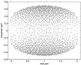
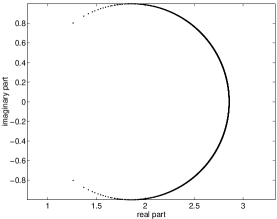
Figure 2: Spectrum of the Wilson fermion matrix $M$ for our $4^{4}$ configuration (left), spectrum of $D_{u}$ for $\mu=0.3$ (right).

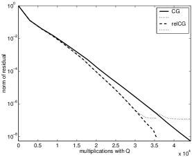
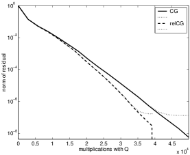
Figure 3: Relaxed and non-relaxed CG for (8). Left: $\mu=0.3$. Right: $\mu=0.1$.

3.2 Numerical illustration

To illustrate the effects of relaxation, we here report on numerical experiments for a simple test situation. More extensive experiments will be reported in Section 5. We use the $4^{4}$ example configuration Conf1 from Section 5, which is the result of a dynamical simulation at $\beta=5.4$. The hopping parameter in the Wilson fermion matrix was taken as $\kappa=0.2$. The spectrum of the Wilson fermion matrix $M$ is given in the left part of Figure 2, the spectrum of the overlap operator $D_{u}$ is plotted on the right. We solved the ‘squared’ equation (8) using the CG method for the mass parameters $\mu=0.3$ and $\mu=0.1$, where $\rho=(1+\mu)/(1-\mu)$, see (15).

The plots in Figure 3 give the norm of the (computed) residual as a function of the number of matrix-vector multiplies (MVMs) with $Q$. These MVMs all occur in the multi-shift CG method when approximating $\hbox{\rm\,sign}(Q)x$ via the Zolotarev approach. Details of our implementation are given in Section 5. Each plot contains two convergence curves, one for CG without relaxation, i.e., with a fixed precision for the MVMs, and one with the relaxed CG method described in Algorithm 1.

In the relaxed CG methods we also used a high accuracy inner iteration for computing the sign function to compare the true and the computed residuals. The true residuals are plotted in Figure 3 as dotted lines. We see that the true and the computed residuals are virtually the same until they are down to $\epsilon=10^{-6}$, the required accuracy, which was the parameter used in (11). We see that the relaxation strategies yield an improvement in the order of 20%, regardless of the value of $\mu$. This improvement is larger in the more realistic computations to be reported in Section 5. There we perform an additional eigenvalue projection step to speed up the overall computation. In this situation relaxation leads to larger gains ranging from 30% to 40%.

4 Further improvements: Recursive preconditioning

In the previous section we discussed strategies for controlling the error of the matrix-vector products. The preliminary numerical experiments there showed that a reduction of at least 20% can be expected compared to the case of using a fixed precision for the matrix-vector products in all steps. Two important practical observations should be made, see also [55, Section 3]. First, we note that, if the number of iterations to reach the desired residual reduction is large, then there can be a considerable accumulation of the errors in the matrix-vector product in the residual gap. This is reflected for the CG method by the fact that the required number of iterations appears in the upper bound on the residual gap in (12) as a factor $k$. In practice, this might mean that the tolerance on the matrix-vectors has to be decreased, which is the tactic taken in [52]. But more importantly, the strategies discussed in the previous section, take the error in the matrix-vector products, essentially, inversely proportional to $\|r^{j}\|$. Krylov subspace methods often show superlinear convergence, meaning that the convergence speed increases as the iterative method proceeds. Hence, the number of inexpensive approximations to the matrix-vector products is relatively small and this limits the maximal gain that can be achieved with the relaxation approach.

Stating the same observation from a different point of view, we conclude that the relaxation strategy should work particularly well when the convergence of the iteration is fast (but linear) from the very beginning. In order to achieve this, we investigate the idea of ‘preconditioning’ the Krylov subspace method by another (inexact) Krylov subspace method set to a larger tolerance of $\xi_{j}$ in step $j+1$. We refer to this as recursive preconditioning.

Figure 4: Overview of our recursive preconditioning computational scheme

To stay consistent with the terminology used so far, we refer to the inexact Krylov method and its variable preconditioner as the outer iteration and preconditioning iteration respectively, reserving the term inner iteration to the method which approximates the matrix vector product. The inner iteration is thus used in both, the preconditioning and the outer iteration, see Figure 4.

Methods that can be used for the outer iteration are the so-called flexible methods. These are methods that are specially designed for dealing with variable preconditioning, e.g., [28, 51, 57]. In [55] these methods were combined with approximate matrix-vector products. For our numerical experiments we chose the GMRESR (GMRES recursive, [57]) method as the outer iteration. Note that other choices like flexible GMRES [51] are an equally good option. We have chosen GMRESR here since it is slightly more straightforward to implement. The paper [55] analyses various choices for the accuracies $\eta_{j}$ and $\xi_{j}$ and shows that $\eta_{j}=\epsilon/\|r^{j}\|$ and $\xi_{j}=\xi$ fixed are good choices. Figure 5 gives a Matlab-style algorithmic description of the overall method, which we call relaxed GMRESR. To stress the preconditioning iteration, we sometimes add it in parenthesis, so that, e.g., relaxed GMRESR(CG) means that we use the CG method as the preconditioning iteration.

Algorithm 2

$\hbox{\rm relGMRESR}(A,b,\epsilon)$

  {computes $x$ with $\|Ax-b\|\leq\epsilon\cdot\|b\|$ via relaxed GMRESR}

  

  $x=0;$   {initial value}

  $r=b;$

  $C=[];$   {empty matrix}

  $U=[];$   {empty matrix}

  while $\|r\|>\epsilon\cdot\|b\|$ do

     solve $Au=r$ to relative accuracy $\xi$ (for example $u=\hbox{\rm relCG}(A,r,\xi);$)

           {preconditioner}

     compute $c$ with $\|Au-c\|\leq\epsilon\cdot\|b\|\cdot\|u\|/\|r\|;$

     for i=1:size(C,2) do

        $\beta=C[:,i]^{\dagger}\cdot c;$

        $c=c-\beta\cdot C[:,i];$

        $u=u-\beta\cdot U[:,i];$

     end for

     $c=c/\|c\|;$

     $u=u/\|c\|;$

     $C=[C,c];$

     $U=[U,u];$

     $\alpha=c^{\dagger}\cdot r;$

     $x=x+\alpha\cdot u;$

     $r=r-\alpha\cdot c;$

  end while

Figure 5: Relaxed GMRESR

The recursive application of iterative solution methods is often encountered in scientific computing applications. For example, van der Vorst and Vuik notice in [57] that preconditioning GMRES with a fixed number of iterations of GMRES can give a considerable improvement over restarted GMRES. This explains the name ‘GMRESR’ which we keep in this paper although we use other choices for the preconditioner.

In the context of approximate matrix-vector products, nested iterations have been used by Carpentieri in his PhD thesis [10]. He uses flexible GMRES in the outer iteration and GMRES in the inner iteration for an application from electromagnetics where the matrix-vector products are approximated using a fast multipole technique set to a fixed precision. The paper [55] shows numerical experiments for a Schur complement system that stems from a model of global ocean circulation. Using the relaxed preconditioned approach one gets a significant reduction in the amount of work spent in the matrix-vector products.

A related idea for the QCD overlap formulation has recently been advanced by Giusti et al. [26, Section 9] in a method which they call an adapted-precision inversion algorithm. Their scheme corresponds to the approach presented here if, instead of GMRESR, one takes a simple Richardson iteration as the outer iteration and if, in addition, the residuals are computed directly. The authors of [26] do not discuss specific choices for the precision of the matrix-vector product in the outer iteration and use a fixed precision in the preconditioning iteration. Our more general approach allows the use of more sophisticated outer iterations like GMRESR and, moreover, gives a specific and computationally feasible strategy on how to choose the precision of the inner iteration.

It is also interesting to mention that the idea of adapted precision inversion is related to an earlier approach of Hernández et al. in [33] and Boriçi in [4].

5 Numerical experiments

Next we present numerical experiments carried out in a realistic setting. To this purpose we have developed a Hybrid Monte-Carlo program (HMC) with either one or two flavours of dynamical overlap fermions based on the Zolotarev partial fraction expansion [53]. Details as to the construction of the overlap fermion force within the HMC can be found in Appendix D.

We have generated decorrelated configurations with one flavour (see Section 5.3 below) of dynamical overlap fermions on an $8^{4}$-lattice at $\beta=5.6$, and with two flavours on a $4^{4}$ lattice at $\beta=5.4$. For our experiments the Wilson kernel mass parameter has been adjusted to $\kappa=0.2$. It is known that the locality properties and spectral density of the overlap operator depend strongly on the value of $\kappa$ used, with $\kappa\sim 0.2$ being the optimum value, at least in the quenched theory on large lattices [34].

We have used a mass parameter $\mu$ [44], which, according to (15), is equivalent to $\rho=(1+\mu)/(1-\mu)$, and we have chosen $\mu=0.1$ ($\rho=1.22$), and $\mu=0.3$ ($\rho=1.857$). These values of $\mu$ are similar to the smallest non-zero eigenvalues of the overlap operator and, given our small lattices, there will be little change in the results when moving $\mu$ to smaller valence mass.

Our results will be given for five configurations for the $4^{4}$ lattice volumes, separated by 50 HMC sweeps, and on three plus five configurations, separated by 20 HMC sweeps on the $8^{4}$ lattice. Additionally, some computations were performed on a configuration from a quenched ($\beta=6.0$) ensemble, with the inversions performed at $\kappa=0.2$, with three values of $\mu$, $0.3$, $0.1$ and $0.03$.

All our computations were carried out on the Wuppertal cluster computer ALiCE, using 16 processors for the calculations on the $8^{4}$ and $16^{4}$ lattices, and one processor for the $4^{4}$ calculations.

5.1 Projecting out low-lying eigenvectors

Let $a$ and $b$ denote the smallest and largest eigenvalue of $Q^{2}$, respectively. Then, in principle, we need the Zolotarev approximation to the sign function for the domain $[-\sqrt{b},-\sqrt{a}]\cup[\sqrt{a},\sqrt{b}]$. As $a$ gets smaller, we need an increasing number of terms in the Zolotarev approximation in order to obtain a given accuracy. It is possible [18] to accelerate the calculation of the sign function by calculating the $n_{p}$ ‘smallest’ eigenvectors of the Wilson operator, and by treating them exactly. The Zolotarev approximation is then only needed on a domain $[-\sqrt{b},-\sqrt{a^{\prime}}]\cup[\sqrt{a^{\prime}},\sqrt{b}]$ with $a^{\prime}$ being not larger than the $n_{p}+1^{\rm st}$ smallest eigenvalue of $Q^{2}$.

Besides from allowing us to shrink the domain over which we need an accurate approximation to the sign function, projecting out small eigenvectors also improves the condition number of the Wilson operator $Q$. As a consequence the multi-mass inversion to be performed for the Zolotarev approximation converges faster.

There are two different ways in which we can project out the eigenvalues – either out of the sign function, or out of the multi-mass solver for the partial fraction expansion. Our preference is to fix $a^{\prime}$ at some suitable value, and to project the eigenvalues below $\sqrt{a^{\prime}}$ directly out of the sign function, and those eigenvalues above $\sqrt{a^{\prime}}$ out of the multi-mass solver [16] (see Appendix C).

We calculate the coefficients of the Zolotarev expansion so that the sign function is approximated to machine precision within the range $[\sqrt{a^{\prime}},\sqrt{b}]$ (see Appendix D). We cannot vary the values of $a^{\prime}$ and $b$ in the outer iteration across the trajectory of the HMC algorithm without violating detailed balance. Some fine tuning of the optimal value of $a^{\prime}$ is possible, but this optimisation lies outside the scope of this paper: here we keep $b$ fixed at $10$, and $a^{\prime}$ fixed at $10^{-5}$. For all the calculations described in this section, we took $n_{p}=28$, which always resulted in a $n_{p}+1^{\rm st}$ smallest eigenvalue larger than $a^{\prime}=10^{-5}$, as required. The performance gain obtained from the eigenvalue projection is briefly described in Appendix C.

In the preconditioner, $b$ and $a^{\prime}$ were allowed to vary. We took $b$ as the largest eigenvalue of $Q^{2}$ (usually around 5), while $a^{\prime}$ was the $n_{p}+1^{\rm st}$ smallest eigenvalue (around $10^{-3}$ for the $4^{4}$ lattices, and $10^{-4}$ for the $8^{4}$ lattices). Since we need the sign function less precise in the preconditioner, the number of poles in the Zolotarev approximation could be taken quite small (see Appendix D), thus minimising the computational effort in the preconditioner.

5.2 Results for the squared overlap operator

Figure 6 gives the convergence history for the third configuration on the $8^{4}$ and the first on the $4^{4}$ lattice. The plots show the residual norm against the numbers of MVMs with the Wilson fermion matrix $Q$. Since the latter dominate the performance of the entire process, we can consider them as a first approximation of the overall execution time. The figure compares the unrelaxed CG, relaxed CG and the relaxed GMRESR(CG) methods. In addition to the plots, we give the actual timings for our implementations in Tables 2-3. Note that for the preconditioned iterations the gain in time is more than the gain obtained in MVMs with $Q$. The reason is that in the preconditioner we only have five different shifts to work on when performing the multi-mass inversion for the Zolotarev approximation, as opposed to the 25 shifts to be used in the outer iteration.

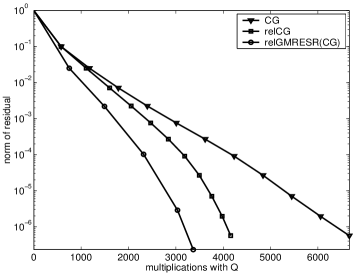
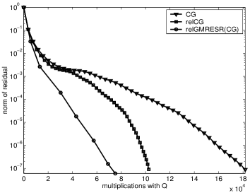
First $4^{4}$, $\mu=0.3$ configuration from table 2 Third $8^{4}$, $\mu=0.1$ configuration from table 3

Figure 6: Convergence history for unrelaxed CG, relaxed CG and relaxed GMRESR for one inversion of the squared equation (2). We plot the norm of the residual vs. the number of calls to the Wilson operator $Q$. The tics indicate each (outer) iteration: On the $4^{4}$ lattice relaxed GMRESR needs 5 iterations to converge, whereas unrelaxed and relaxed CG both require 11 iterations.

Comparing the times from the tables we see that on the $8^{4}$ lattices relaxation already reduces the computational effort by a factor of 1.7. Additional preconditioning further reduced the effort by an additional factor of 2.2 (taking $\xi_{j}=\xi=0.1$ independently of $j$ since there was little change in the gain for $0.01<\xi_{j}<0.3$).

The gain turned out to be smaller on the $4^{4}$ ensembles, with only about a factor of 1.5 gain for the relaxation, and an additional factor of 1.3 for the preconditioner. The gain on the $16^{4}$ quenched configuration is similar to the gain for the $8^{4}$ ensembles. The lower gain for the preconditioner on the smaller lattices is due to the fact that the CG inversion on $4^{4}$ lattices converges already quite fast, a consequence of the particular eigenvalue distribution of the $4^{4}$ lattice already observed in Figure 2. Thus, the $4^{4}$ inversion spent more time in the outer GMRESR algorithm (compared to the time spent in the CG preconditioner) than the $8^{4}$ inversion did. Since one sweep through the GMRESR algorithm takes considerably longer than one sweep through the CG preconditioner, this reduced the gain of the preconditioning on the smallest lattices. For the same reason, the gain achieved by preconditioning is larger as we decrease the overlap mass, especially on the larger lattices, where the overlap operator is less well conditioned. For example, on the $16^{4}$ quenched configuration, the gain for using the preconditioner is 1.75 times larger for $\mu=0.03$ than for $\mu=0.3$.

Method	Conf 1	Conf 2	Conf 3	Conf 4	Conf 5
CG	53	55	53	57	55
relCG	34(1.56)	35(1.57)	36(1.47)	37(1.54)	38(1.45)
relGMRESR(CG)	19(2.78)	20(2.75)	24(2.21)	25(2.28)	26(2.11)

$\mu=0.3$

Method	Conf 1	Conf 2	Conf 3	Conf 4	Conf 5
CG	50	46	44	46	48
relCG	33(1.52)	31(1.48)	30(1.47)	32(1.44)	31(1.55)
relGMRESR(CG)	22(2.27)	20(2.30)	23(1.91)	25(1.84)	21(2.29)

$\mu=0.1$

Table 2: Times (in seconds) for one inversion on the five $4^{4}$ configurations with $\beta=5.4$, run on 1 processor of ALiCE. The number in brackets is the gain from the unrelaxed and unpreconditioned (CG) inversion.

Method	Conf 1	Conf 2	Conf 3	Conf 4	Conf 5
CG	1419	1139	1216	1307	1305
relCG	754(1.88)	697(1.63)	737(1.65)	816(1.60)	767(1.70)
relGMRESR(CG)	319(4.45)	301(3.78)	315(3.86)	364(3.59)	341(3.82)

$\mu=0.3$

Method	Conf 1	Conf 2	Conf 3
CG	1965	2052	2039
relCG	1202(1.63)	1250(1.64)	1234(1.65)
relGMRESR(CG)	614(3.20)	567(3.61)	547(3.72)

$\mu=0.1$

Table 3: Times (in seconds) for one inversion on the three $8^{4}$ configurations with $\beta=5.6$, run on 16 processors of ALiCE.

Method	$\mu=0.03$	$\mu=0.1$	$\mu=0.3$
CG	31430	9022	3493
relCG	18813(1.67)	5981(1.51)	2610(1.34)
relGMRESR(CG)	6642(4.73)	2329(3.87)	1286(2.71)

Table 4: Times (in seconds) for one inversion on the quenched $16^{4}$ configuration at $\beta=6.0$, run on 16 processors of ALiCE.

5.3 Chiral projection.

Based on investigations of the Schwinger model, the authors of [2] suggested that it might be beneficial to project the squared overlap operator to one chiral sector. We have

$$D_{h}^{2} = D_{+}^{2}+D_{-}^{2};$$

$$D_{\pm}^{2} = \frac{1}{2}D_{h}^{2}\left(I\pm\gamma_{5}\right)$$

$$= \frac{\rho^{2}+1}{2}\left(I\pm\gamma_{5}\right)\pm\frac{\rho}{2}\left(I\pm\gamma_{5}\right)\hbox{\rm\,sign}(Q)\left(I\pm\gamma_{5}\right).$$

Because $[D_{h}^{2},\gamma_{5}]=0$, the eigenvalues, $(\lambda^{h}_{j\pm})^{2}$ of $D_{\pm}^{2}$ are the same, except for the zero modes and their partners. If there are no zero modes then

$$\det D_{u}=\det D_{+}^{2}=\det D_{-}^{2},$$

since the non-zero eigenvalues of $D_{u}$ are

$$\lambda_{j\pm}^{u}=\frac{(\lambda^{h}_{j})^{2}}{2\rho}-\frac{1-\rho^{2}}{2\rho}\pm i\sqrt{(\lambda^{h}_{j})^{2}-\left(\frac{(\lambda^{h}_{j})^{2}}{2\rho}-\frac{1-\rho^{2}}{2\rho}\right)^{2}}.$$

Zero modes can be treated exactly at the end of the simulation by re-weighting the observables according to $(2(1-\rho)/(1+\rho))^{|Q_{f}|N_{f}}$, where $Q_{f}$ is the fermionic topological charge. This means that we can run $N_{f}=1$ simulations by projecting $\phi$ into one chiral sector and running the HMC with $D_{+}^{2}$ rather than $D_{h}^{2}$. The calculation of $D_{\pm}^{2}$ only requires one call to the sign function rather than two, so in principle working in one chiral sector should run an $N_{f}=1$-simulation in half the time it takes to run an $N_{f}=2$-simulation without the projection.

There are two advantages in using the chiral projection. Firstly, we can work in the topological sector that contains no zero-modes, which means that the inverse of the Dirac operator exists even at $\rho=1$ ($\mu=0$). The convergence of the inversion should be improved when the fermion mass is of the same size as the smallest non-zero eigenvalues. It is however unlikely that on more realistic lattice sizes that we will be able to run at small enough masses to see such an effect.

Secondly, and more importantly, it should allow more frequent changes of the topological charge in the chiral sector opposite to the one we are working in, which means that better samples in configuration space and reduction of the autocorrelation time can be achieved. This effect was seen in the Schwinger model  [2], and our early results suggest that it is present in four dimensions as well. In fact, HMC runs without chiral projection are very resistant to changes in the topological charge.

However, there is also a disadvantage with this method. At low fermion masses, the $Q_{f}=0$ configurations will dominate the statistical average. As a consequence $Q_{f}\neq 0$ configurations will turn out to be relatively unimportant. Whether these disadvantages outweigh the advantages is an open question. However, even if it is not advantageous to use chiral projection for the up and down quark contributions to the determinant, it would certainly be a useful tool if we wish to include a dynamical strange quark in a $N_{f}=3$ simulation.

Method	Conf 1	Conf 2	Conf 3	Conf 4	Conf 5
CG	631	564	623	635	641
relCG	399(1.58)	362(1.56)	399(1.56)	413(1.54)	398(1.61)
relGMRESR(CG)	190(3.32)	171(3.30)	180(3.46)	199(3.19)	181(3.54)

Table 5: Times (in seconds) for the inversion of chiral fermions on the $8^{4},$ $\mu=0.3$ ensemble, run on 16 processors of ALiCE

Table 5 summarises results for these chiral projection computations with $D^{2}_{+}$ on the $8^{4}$ configurations with $\mu=0.1$. Since $D^{2}_{+}$ is hermitian positive definite, the unrelaxed and relaxed computations were done with CG. The preconditioned variant took relaxed GMRESR as the outer iteration with the CG iteration being the preconditioner. There is, as expected, an overall gain of a factor of approximately 2 for the chirally projected inversion, which is due to the fact that we only need to call the sign function once for each application of the squared overlap operator. This gain will not appear in any HMC simulation, since we need to run two such inversions to get a $N_{F}=2$ ensemble. However, single-flavour simulations come for free in this framework. Again, the gain from relaxation and preconditioning is between 3 and 4, although the gain from relaxation and preconditioning is slightly smaller when chiral projection is used (compare Table  5 and  3).

5.4 The two pass SUMR inversion and propagator calculations.

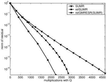
first $4^{4},\mu=0.3$ configuration from Table 2 third $8^{4},\mu=0.1$ configuration from Table 3

Figure 7: Convergence history for unrelaxed SUMR, relaxed SUMR and relaxed GMRESR(SUMR), two pass strategy for (2)

In a last series of investigations, we performed two pass computations (see Section 2.2) on the $8^{4}$ and $4^{4}$ configurations. We now compare unrelaxed SUMR, relaxed SUMR and relaxed GMRESR(SUMR), i.e. the preconditioning is done with SUMR. As before, we required a fixed accuracy $\xi_{j}=\xi=0.1$ in the preconditioning iteration. As can be seen in Figure 7 and Tables 6 to 8, there is again an improvement of around a factor of 3 to 4 when relaxation and preconditioning are used, and again this factor increases as we decrease $\mu$, especially on the larger lattices. In [1], we predicted that two passes through SUMR should theoretically take roughly the same time as one pass through CG, although in numerical tests we found that the two pass method was slightly slower. Comparing Tables 6 to 8 and Tables 2 to 3, we can see that as we move to larger lattices the unrelaxed two pass strategies do take approximately the same time as the single CG inversion. However, the gain in using the preconditioner is generally larger for the SUMR inversion than for the CG inversion. If this trend continues, then as we move to larger dynamical simulations, it might be preferable to use the two pass strategy to calculate the HMC fermionic force. Indeed, on our $16^{4}$ quenched configuration at the lower masses, two SUMR inversions already improve upon one CG inversion when we use the preconditioning technique.

To calculate the propagator we need to perform a single inversion of the overlap operator using SUMR. The time needed for this calculation will be half the time for the two pass inversions described in this section.

Method	Conf 1	Conf 2	Conf 3	Conf 4	Conf 5
SUMR	68	59	59	66	63
relSUMR	48(1.42)	41(1.44)	41(1.44)	45(1.47)	44(1.43)
relGMRESR(SUMR)	25(2.72)	24(2.46)	23(2.57)	32(2.06)	29(2.17)

$\mu=0.3$

Method	Conf 1	Conf 2	Conf 3	Conf 4	Conf 5
SUMR	88	87	89	89	94
relSUMR	60(1.47)	61(1.43)	59(1.51)	64(1.39)	66(1.42)
relGMRESR(SUMR)	23(3.82)	21(4.14)	28(3.18)	30(2.97)	34(2.76)

$\mu=0.1$

Table 6: Times (in seconds) for two SUMR inversions on the five $4^{4}$ configurations at $\beta=5.4$, run on one processor of ALiCE.

Method	Conf 1	Conf 2	Conf 3	Conf 4	Conf 5
SUMR	1538	1181	1222	1288	1286
relSUMR	804(1.91)	748(1.58)	795(1.54)	818(1.57)	796(1.62)
relGMRESR(SUMR)	383(4.02)	351(3.36)	383(3.19)	392(3.28)	382(3.37)

$\mu=0.3$

Method	Conf 1	Conf 2	Conf 3
SUMR	2272	2685	2510
relSUMR	1695(1.34)	1661(1.62)	1500(1.67)
relGMRESR(SUMR)	674(3.38)	650(4.13)	576(4.36)

$\mu=0.1$

Table 7: Times (in seconds) for two SUMR inversions on the $8^{4}$ configurations at $\beta=5.6$, run on 16 processors of ALiCE.

Method	$\mu=0.03$	$\mu=0.1$	$\mu=0.3$
SUMR	31550	8312	3200
relSUMR	18840(1.87)	6038(1.38)	2656(1.20)
relGMRESR(SUMR)	5974(5.82)	2252(3.69)	1382(2.32)

Table 8: Times (in seconds) for two SUMR inversions on the quenched $16^{4}$ configuration, run on 16 processors of ALiCE.

6 Discussion

Ginsparg-Wilson fermions, such as overlap fermions, offer an intriguing possibility to overcome the bottleneck which affects dynamical simulations with Wilson fermions at light quark masses. The lattice chiral symmetry satisfied by the Ginsparg-Wilson fermions will also enable us to study aspects of QCD such as chiral symmetry breaking and topology better than it is possible with Wilson fermions.

The bottleneck of dynamical simulations with Ginsparg-Wilson fermions is the computational time. In order to invert the overlap operator in the course of the Monte-Carlo simulation, we need to run a nested inversion, which means that overlap fermions are of the order $\mathcal{O}(100)$ times as expensive as Wilson fermions. The hope is that by improving algorithmic techniques we can bring the computational cost down to something manageable. In this paper, we have studied two such techniques – relaxation of the accuracy of the inner inversion, and using a low accuracy approximation of the sign function in a preconditioner. Considering the results on the $4^{4}$ lattices less typical, we conclude that these techniques lead to a factor of $3$ to $4$ improvement in the computational effort required to invert the overlap operator. Improvements tend to be even better for more demanding computations, i.e. when $\mu$ becomes smaller. Our approach comes on top of the more classical eigenvector projection-techniques, to which it contributes its improvements in a multiplicative manner.

Using the techniques outlined in this paper (and anticipating further improvements), we hope to be able to run HMC algorithms using overlap fermions on moderate lattice sizes on the next generation of cluster computers. There are some subtleties when running the HMC algorithm with overlap functions, the most notable being that the derivative of the sign function generates a step function in the fermionic force. We plan to discuss the Hybrid Monte-Carlo algorithm in more detail and present some initial results on small lattices in a subsequent paper.

7 Acknowledgements

N.C. enjoys support from the EU Research and Training Network HPRN-CT-2000-00145 “Hadron Properties from Lattice QCD”, and EU Marie-Curie Grant number MC-EIF-CT-2003-501467. A.F. and K.S. acknowledge support by DFG under grant Fr755/17-1. We thank Guido Arnold for his help in an early stage of this project. We are grateful to Norbert Eicker and Boris Orth for their help with the cluster computer ALiCE at Wuppertal University.

Appendix A Definitions

The Wilson-Dirac matrix reads:

$$M_{nm}=\delta_{nm}-\kappa D_{W},$$

where the hopping term is defined as

$$D_{W}=\sum_{\mu}(1-\gamma_{\mu})U_{\mu}(n)\delta_{n,m-\mu}+(1+\gamma_{\mu})U^{\dagger}_{\mu}(n-\mu)\delta_{n,m+\mu}.$$ (13)

$\kappa$ is the hopping parameter, which is defined as $\kappa=1/(8-2m_{0})$, where $m_{0}$ is the Wilson mass. The hermitian Euclidean $\gamma$ matrices satisfy the anti-commutation relation $\left\{\gamma_{i},\gamma_{j}\right\}=2\delta_{ij}$ $i,j=1,\ldots 4$. $\gamma_{5}$ is the product $\gamma_{5}=\gamma_{1}\gamma_{2}\gamma_{3}\gamma_{4}$, which means that $\left\{\gamma_{5},\gamma_{\mu}\right\}=0$. The hermitian form of the Wilson-Dirac matrix is given by multiplication of $M$ with $\gamma_{5}$:

$$Q=\gamma_{5}\,M.$$ (14)

Appendix B Massive Overlap Operator

Following Neuberger  [44], one can write the massive overlap operator as

$$D_{u}(\mu)=c\left((1+\mu)+(1-\mu)\gamma_{5}\hbox{\rm\,sign}(Q)\right).$$

The normalisation $c$ can be absorbed into the fermion renormalisation, and will not contribute to any physics. For convenience, we have set $c=1$. Thus, the regularising parameter $\rho$ as defined in (1) is related to $\mu$ by

$$\rho=(1+\mu)/(1-\mu).$$ (15)

The mass of the fermion is given by

$$m_{f}=Z_{m}\frac{2\mu m_{0}}{(1-\mu)},$$

where $Z_{m}$ is a renormalisation factor.

Another form of the massive overlap operator, which sometimes appears in the literature (e.g. in  [14]), is

$$D_{u}=m+(m_{0}-\frac{1}{2}m)(1+\gamma_{5}\hbox{\rm\,sign}(Q)).$$

This is equivalent to the formula which we use, with $\mu=m/(2m_{0})$.

Appendix C Projection of low lying eigenvectors

It is advantageous to project out the low lying eigenvectors of the Wilson operator $Q$ when calculating the sign function [18] (see Table 9). Let the eigenvalues of $Q^{2}$ be contained in $[a,b]$. The smallest eigenvalues of $Q$ can be projected out of the sign function and out of the multi-mass inversion used to calculate the rational fraction [16]. We take the Zolotarev approximation with respect to a domain $[-\sqrt{b},-\sqrt{a^{\prime}}]\cup[\sqrt{a^{\prime}},\sqrt{b}]$ where $a^{\prime}\geq a$. Beforehand, we compute a set $\Lambda$ of the $n_{p}$ smallest eigenvalues of $Q$ and partition $\Lambda=\Lambda_{1}\cup\Lambda_{2}$ where $\Lambda_{2}$ contains those eigenvalues which are larger in modulus than $a^{\prime}$. If $\psi^{\lambda}$ are the normalised eigenvectors of the eigenvalues $\lambda$ with respect to which we project, then

$$\text{sign}(Q)x=\text{sign}(Q)\left(x-\sum_{\lambda\in\Lambda_{1}}\psi^{\lambda}(\psi^{\lambda},x)\right)+\sum_{\lambda\in\Lambda_{1}}\text{sign}(\lambda)\psi^{\lambda}(\psi^{\lambda},x).$$

This shows that in order to compute $\hbox{\rm\,sign}(Q)x$ we need the Zolotarev approximation only on the range $[-\sqrt{b},-\sqrt{a^{\prime}}]\cup[\sqrt{a^{\prime}},\sqrt{b}]$.

The projection approach in the subsequent multi-mass solver is to solve

$$\left(\frac{1}{{a^{\prime}}}Q^{2}+\tau_{i}\right)^{-1}y= \left(\frac{1}{{a^{\prime}}}Q^{2}+\tau_{i}\right)^{-1}\left(y-\sum_{\lambda\in\Lambda_{2}}\psi^{\lambda}(\psi^{\lambda},y)\right)+$$

$$\sum_{\lambda\in\Lambda_{2}}\frac{1}{\frac{1}{{a^{\prime}}}\lambda^{2}+\tau_{i}}\psi^{\lambda}(\psi^{\lambda},y),$$

where $y=x-\sum_{\lambda\in\Lambda_{1}}\psi^{\lambda}(\psi^{\lambda},x)$.

This eigenvector projection improves the condition number of the inversion, and therefore the CG method will converge faster. Note that projecting all computed eigenvalues directly out of the sign function would allow us to use a larger lower bound $a^{\prime}$ for the Zolotarev expansion which will speed up the calculation further. However, this comes with an additional cost when calculating the fermionic force, and our preference is to only use this method for exceptionally small eigenvalues. Furthermore, in order to satisfy detailed balance, we need to use the same Dirac operator throughout the calculation, i.e. we are forced to keep $a^{\prime}$ fixed.

$n_{p}$	Inversion	Calls to Wilson op.	Eigenvalue calculation	Total time
1	9144	1032172	0	9144
10	1269	189514	111	1380
20	796	112862	118	914
30	568	78548	172	740
40	459	63566	274	733
50	387	52758	361	748
60	340	45732	410	750

Table 9: The times (in seconds) needed to calculate one relGMRESR(CG) inversion of the overlap operator, and to calculate $n_{p}$ eigenvalues of the Wilson operator for different values of $n_{p}$, on the $8^{4}$ configuration 1 with $\mu=0.1$.

$n_{p}$	Inversion	Calls to Wilson op.	Eigenvalue calculation	Total time
1	131	13112	18	149
10	30	4860	14	44
20	24	3532	22	46
30	19	2874	31	50
40	17	2474	60	77

Table 10: The times (in seconds) needed to calculate one relGMRESR(CG) inversion of the overlap operator, and to calculate $n_{p}$ eigenvalues of the Wilson operator for different values of $n_{p}$, on the $4^{4}$ configuration 1, with $\mu=0.1$.

The eigenvectors have to be calculated every time the gauge field is updated. In an HMC algorithm this means that the time taken for each micro-canonical step is the sum of the time taken for the calculation of the eigenvectors and the time needed for the inversion of the overlap operator (the calculation of the remainder of the fermionic force is negligible). Some fine tuning of $n_{p}$, the number of eigenvectors projected out, is therefore required. We used an Arnoldi algorithm with Chebyshev improvement to calculate the lowest eigenvalues of the squared Wilson operator [43]. From Tables 9 and 10, we can see that there is a factor of 3 gain in using the eigenvalue projection on the smaller lattices, and there is a large factor of 12 on the larger lattices.

Appendix D Hybrid Monte-Carlo with Overlap Fermions

D.1 The Zolotarev approximation.

We approximate the action of the matrix sign function $\hbox{\rm\,sign}(Q)=\gamma_{5}M(M^{\dagger}M)^{-\frac{1}{2}}$ on a vector $y$ using the Zolotarev rational approximation. This ($l_{\infty}$) best approximation $r(\lambda)$ to $\hbox{\rm\,sign}(\lambda)$ on $[-\sqrt{b},-\sqrt{a}]\cup[\sqrt{a},\sqrt{b}]$ is given as [50]

$$\hbox{\rm\,sign}(\lambda)\sim r(\lambda)=\lambda\cdot D\cdot\frac{\prod_{j=1}^{N_{Z}-1}\left(\lambda^{2}+c_{2j}\right)}{\prod_{j=1}^{N_{Z}}\left(\lambda^{2}+c_{2j-1}\right)},$$ (16)

where the coefficients are constructed using elliptic integrals as

$$c_{j}= \frac{\text{sn}^{2}\left(jK/(2N_{Z});\kappa\right)}{1-\text{sn}^{2}\left(jK/(2N_{Z});\kappa\right)}$$

$$K= \int_{0}^{1}\frac{dt}{\sqrt{(1-t^{2})(1-\kappa^{2}t^{2})}}$$

$$\kappa= \sqrt{1-\frac{a}{b}}.$$

$D$ is uniquely defined via the relation

$$\max_{\lambda\in[\sqrt{a},\sqrt{b}]}\left(1-\sqrt{\lambda}r(\lambda)\right)=-\min_{\lambda\in[\sqrt{a},\sqrt{b}]}\left(1-\sqrt{\lambda}r(\lambda)\right).$$

The rational function $r(\lambda)$ in (16) can equivalently be represented by its partial fraction expansion

$$r(\lambda)= \frac{1}{\sqrt{a}}\cdot\lambda\cdot\sum_{j=1}^{N_{Z}}\omega_{j}\left(\frac{1}{a}\lambda^{2}+\tau_{j}\right)^{-1}$$

where

$$\omega_{j} = \frac{\prod_{k=1}^{n-1}(c_{2j-1}-c_{2k})}{\prod_{k\neq j,k=1}^{k=n}(c_{2j-1}-c_{2k-1})}$$

$$\tau_{j} = c_{2j-1}$$

Using this representation, we approximate the action of the matrix sign function on a vector $y$ as

$$\hbox{\rm\,sign}(Q)y\sim \frac{1}{\sqrt{a}}Q\sum_{j=1}^{N_{Z}}\omega_{j}A_{j}y,\quad\mbox{ where $A_{j}=\left(\frac{1}{a}Q^{2}+\tau_{j}I\right)^{-1}$}.$$

Herein, the $y^{j}=A_{j}y$ are calculated using the multi-shift CG method [23, 39] as a multi-mass inverter for the systems $\left(\frac{1}{a}Q^{2}+\tau_{j}I\right)y^{j}=y$. For the outer iteration we set the order of the Zolotarev expansion to be $N_{Z}=25$, which gave the sign function accurate to machine precision when the multi-mass solver was calculated to machine precision. When we needed less precision in the relaxed methods, we stopped the multi-mass solver earlier, see [53]. When evaluating the sign function in a preconditioner, where we only required an accuracy of $10^{-1}$, we could reduce the order of the expansion to $N_{Z}=5$.

D.2 The fermionic force.

The fermionic part of the Hybrid Monte-Carlo action is given by

$$S_{pf}= \phi^{\dagger}X;\qquad X=(H_{N})^{-2}\phi.$$

The fermionic force needed for the Hybrid Monte-Carlo algorithm at a lattice site $x$ and direction $\mu$ is

$$F_{\mu}(x)= (1-\mu^{2})\left(X^{\dagger}\gamma_{5}\right)_{n}\left(F^{R}_{\mu,nm}(b)+F^{P}_{\mu,nm}(x)+F^{S}_{\mu,nm}(x)\right)X_{m}$$

$$(1-\mu^{2})X^{\dagger}_{n}\left(F^{R}_{\mu,nm}(x)+F^{P}_{\mu,nm}(x)+F^{S}_{\mu,nm}(x)\right)\left(\gamma_{5}X\right)_{m}$$

$$F^{R}_{\mu,nm}(x)= \kappa\frac{1}{\sqrt{a}}\omega_{\eta}A^{k}_{nb}\left[\frac{1}{a}Q_{bx}\gamma_{5}(1-\gamma_{\mu})\delta_{x+\mu,c}Q_{cd}-\right.$$

$$\left.\tau_{k}\gamma_{5}(1-\gamma_{\mu})\delta_{b,x}\delta_{x+\mu,d}\right]A^{k}_{de}\left(1-\left|\psi^{\lambda}\right\rangle\left\langle\psi^{\lambda}\right|\right)_{em}$$

$$F^{P}_{\mu,nm}(x)= -\kappa\left(\frac{1}{\sqrt{a}}\frac{Q\omega_{k}}{\frac{1}{a}Q^{2}+\tau_{k}}\right)_{nb}P_{\lambda bx}\gamma_{5}(1-\gamma_{\mu})\delta_{x-e_{\mu},c}\left(\left|\psi^{\lambda}\right\rangle\left\langle\psi^{\lambda}\right|\right)_{cm}$$

$$-\kappa\left(\frac{1}{\sqrt{a}}\frac{\frac{1}{a}Q\omega_{k}}{Q^{2}+\tau_{k}}\right)_{na}\left(\left|\psi^{\lambda}\right\rangle\left\langle\psi^{\lambda}\right|\right)_{bx}\gamma_{5}(1-\gamma_{\mu})\delta_{x,c+e_{\mu}}P_{\lambda cm}$$

$$F^{S}_{\mu,nm}(x)= \kappa P_{\lambda nx}\gamma_{5}\hbox{\rm\,sign}(\lambda)(1-\gamma_{\mu})\delta_{x,c+e_{\mu}}\left(\left|\psi^{\lambda}\right\rangle\left\langle\psi^{\lambda}\right|\right)_{cm}+$$

$$\kappa\left(\left|\psi^{\lambda}\right\rangle\left\langle\psi^{\lambda}\right|\right)_{nx}\gamma_{5}(1-\gamma_{\mu})\delta_{x,c+e_{\mu}}\epsilon(\lambda)P_{\lambda cm}-$$

$$\left(\left|\psi^{\lambda}\right\rangle\left\langle\psi^{\lambda}\right|\right)_{nm}\frac{d}{d\lambda}\hbox{\rm\,sign}(\lambda)\left\langle\psi^{\lambda}\right|_{x}\gamma_{5}(1-{\gamma_{\mu}})\delta_{x,c+e_{\mu}}\left|\psi^{\lambda}\right\rangle_{c}$$

$$P_{\lambda}= (1-\left|\psi^{\lambda}\right\rangle\left\langle\psi^{\lambda}\right|)(Q-\lambda)^{-1}(1-\left|\psi^{\lambda}\right\rangle\left\langle\psi^{\lambda}\right|).$$

We assume summations over all repeated indices, including sums over all the projected eigenvectors. Note that the fermionic force contains a delta function in the smallest eigenvalue. This means that if the smallest eigenvalue changes sign during the molecular dynamics of the Hybrid Monte-Carlo, then some care needs to be taken when calculating the fermionic force. We will discuss this matter fully, and present our solution to the problem, in a future publication [16] (see also [21]).

In order to calculate the fermionic force, we need to perform two multi-mass inversions of the Wilson operator and one inversion of the squared overlap operator (e.g. by using relGMRESR(CG)). As discussed during this paper, it is this second step which is time-consuming. We also need to calculate $S_{pf}$ during the Monte-Carlo process, and for this we require just a single inversion of the overlap operator (e.g. by using relGMRESR(SUMR)).

References

- [1] G. Arnold, N. Cundy, J. van den Eshof, A. Frommer, S. Krieg, Th. Lippert, and K. Schäfer, Numerical methods for the QCD overlap operator: II. optimal Krylov subspace methods, (2003), hep-lat/0311025.
- [2] A. Bode, U. M. Heller, R. G. Edwards, and R. Narayanan, First experiences with HMC for dynamical overlap fermions, Dubna 1999, Lattice fermions and structure of the vacuum, 1999, hep-lat/9912043, pp. 65–68.
- [3] A. Boriçi, On the Neuberger overlap operator, Phys. Lett. B453 (1999), 46–53, hep-lat/9810064.
- [4] , Chiral fermions and multigrid, Phys. Rev. D62 (2000), 017505, hep-lat/9907003.
- [5] , Fast methods for computing the Neuberger operator, in Frommer et al. [22], Proceedings of the International Workshop, University of Wuppertal, August 22-24, 1999, pp. 40–47.
- [6] , A Lanczos approach to the inverse square root of a large and sparse matrix, J. Comput. Phys. 162 (2000), 123, hep-lat/9910045.
- [7] A. Bouras and V. Frayssé, A relaxation strategy for inexact matrix-vector products for Krylov methods, Technical Report TR/PA/00/15, CERFACS, France, 2000.
- [8] A. Bouras, V. Frayssé, and L. Giraud, A relaxation strategy for inner-outer linear solvers in domain decomposition methods, Technical Report TR/PA/00/17, CERFACS, France, 2000.
- [9] B. Bunk, Fractional inversion in Krylov space, 1998, hep-lat/9805030.
- [10] B. Carpentieri, Sparse preconditioners for dense complex linear systems in electromagnetic applications, Ph.D. dissertation, INPT, April 2002, TH/PA/02/48.
- [11] T. Chiu, Locality of optimal lattice domain-wall fermions, Phys. Lett. B552 (2003), 97–100, hep-lat/0211032.
- [12] , Optimal domain-wall fermions, Phys. Rev. Lett. 90 (2003), 071601.
- [13] , Optimal lattice domain-wall fermions with finite n(s), 2003, hep-lat/0304002.
- [14] T. Chiu and T. Hsieh, Light quark masses, chiral condensate and quark-gluon condensate in quenched lattice QCD with exact chiral symmetry, 2003, To appear in Nucl. Phys. B, hep-lat/0305016.
- [15] T. Chiu, T. Hsieh, C. Huang, and T. Huang, A note on the Zolotarev optimal rational approximation for the overlap Dirac operator, phys. Rev. D66 (2002), 114502, hep-lat/0206007.
- [16] N. Cundy, S. Krieg, A. Frommer, T. Lippert, and K. Schilling, Numerical methods for the QCD overlap operator: IV. hybrid Monte-Carlo with overlap fermions., In preparation.
- [17] S. J. Dong et al., Chiral logs in quenched QCD, 2003, hep-lat/0304005.
- [18] R. G. Edwards, U. M. Heller, J. Kiskis, and R. Narayanan, Topology and chiral symmetry in QCD with overlap fermions, Dubna 1999, Lattice fermions and structure of the vacuum, 1999, hep-lat/9912042, pp. 53–64.
- [19] , Chiral condensate in the deconfined phase of quenched gauge theories, Phys. Rev. D61 (2000), 074504, hep-lat/9910041.
- [20] R. G. Edwards, U. M. Heller, and R. Narayanan, A study of practical implementations of the overlap-Dirac operator in four dimensions, Nucl. Phys. B540 (1999), 457–471, hep-lat/9807017.
- [21] Z. Fodor, S. Katz, and K. K. Szabo, Dynamical overlap fermions, results with hybrid Monte-Carlo algorithm, hep-lat/0311010.
- [22] A. Frommer, Th. Lippert, B. Medeke, and K. Schilling (eds.), Numerical challenges in lattice quantum chromodynamics, Lecture Notes in Computational Science and Engineering, Springer Verlag, Heidelberg, 2000, Proceedings of the International Workshop, University of Wuppertal, August 22-24, 1999.
- [23] A. Frommer and P. Maass, Fast CG-based methods for Tikhonov-Phillips regularization, SIAM J. Sc. Comput. 20 (1999), 1831–1850.
- [24] R. V. Gavai, S. Gupta, and R. Lacaze, Speed and adaptability of overlap fermion algorithms, Comput. Phys. Commun. 154 (2003), 143–158, hep-lat/0207005.
- [25] P. H. Ginsparg and K. G. Wilson, A remnant of chiral symmetry on the lattice, Phys. Rev. D25 (1982), 2649.
- [26] L. Giusti, C. Hoelbling, M. Lüscher, and H. Wittig, Numerical techniques for lattice QCD in the - regime, Comput. Phys. Commun. 153 (2003), 31–51, hep-lat/0212012.
- [27] L. Giusti, C. Hoelbling, and C. Rebbi, Light quark masses with overlap fermions in quenched QCD, Phys. Rev. D64 (2001), 114508, hep-lat/0108007.
- [28] G. H. Golub and M. L. Overton, The convergence of inexact Chebyshev and Richardson iterative methods for solving linear systems, Numer. Math. 53 (1988), no. 5, 571–593. MR 90b:65054
- [29] G. H. Golub, Z. Zhang, and H. Zha, Large sparse symmetric eigenvalue problems with homogeneous linear constraints: the Lanczos process with inner-outer iterations, Linear Algebra Appl. 309 (2000), no. 1-3, 289–306. MR 2001e:65060
- [30] A. Greenbaum, Iterative methods for solving linear systems, Frontiers in Applied Mathematics, vol. 17, Society for Industrial and Applied Mathematics (SIAM), Philadelphia, PA, 1997. MR 98j:65023
- [31] P. Hasenfratz, Prospects for perfect actions., Nucl.Phys.Proc.Suppl. 63 (1998), 53–58, hep-lat/9709110.
- [32] P. Hernández, K. Jansen, and L. Lellouch, Finite-size scaling of the quark condensate in quenched lattice QCD, Phys. Lett. B469 (1999), 198–204, hep-lat/9907022.
- [33] P. Hernández, K. Jansen, and L. Lellouch, A numerical treatment of Neuberger’s lattice Dirac operator, in Frommer et al. [22], Proceedings of the International Workshop, University of Wuppertal, August 22-24, 1999, pp. 29–39.
- [34] P. Hernández, K. Jansen, and M. Lüscher, Locality properties of Neuberger’s lattice Dirac operator, Nucl. Phys. B552 (1999), 363–378, hep-lat/9808010.
- [35] P. Hernández, K. Jansen, and M. Lüscher, A note on the practical feasibility of domain-wall fermions, hep-lat/0007015, 2000.
- [36] Pilar Hernández, K. J., and L. Lellouch, Chiral symmetry breaking from Ginsparg-Wilson fermions, Nucl. Phys. Proc. Suppl. 83 (2000), 633–635, hep-lat/9909026.
- [37] C. F. Jagels and L. Reichel, A fast minimal residual algorithm for shifted unitary matrices, Numer. Linear Algebra Appl. 1 (1994), no. 6, 555–570. MR 95j:65030
- [38] K. Jansen, Overlap and domain wall fermions: What is the price of chirality?, Nucl. Phys. Proc. Suppl. 106 (2002), 191–192, hep-lat/0111062.
- [39] B. Jegerlehner, Krylov space solvers for shifted linear systems, (1996), hep-lat/9612014.
- [40] M. Lüscher, Abelian chiral gauge theories on the lattice with exact gauge invariance, Nucl. Phys. B549 (1999), 295–334, hep-lat/9811032.
- [41] Y. Namekawa et al., Light hadron spectroscopy in two-flavor qcd with small sea quark masses, (2004).
- [42] R. Narayanan and H. Neuberger, An alternative to domain wall fermions, Phys. Rev. D62 (2000), 074504, hep-lat/0005004.
- [43] H. Neff, Efficient computation of low-lying eigenmodes of non- hermitian Wilson-Dirac type matrices, Nucl. Phys. Proc. Suppl. 106 (2002), 1055–1057, hep-lat/0110076.
- [44] H. Neuberger, Vector like gauge theories with almost massless fermions on the lattice, Phys. Rev. D57 (1998), 5417–5433, hep-lat/9710089.
- [45] , Overlap Dirac operator, in Frommer et al. [22], Proceedings of the International Workshop, University of Wuppertal, August 22-24, 1999, pp. 1–17.
- [46] Herbert Neuberger, Exactly massless quarks on the lattice, Phys. Lett. B417 (1998), 141–144.
- [47] , More about exactly massless quarks on the lattice, Phys. Lett. B427 (1998), 353–355.
- [48] , A practical implementation of the overlap-dirac operator, Phys. Rev. Lett. 81 (1998), 4060–4062.
- [49] , Vector like gauge theories with almost massless fermions on the lattice, Phys. Rev. D57 (1998), 5417–5433.
- [50] P. P. Petrushev and V. A. Popov, Rational approximation of real functions, Cambridge University Press, Cambridge, 1987. MR 89i:41022
- [51] Y. Saad, A flexible inner-outer preconditioned GMRES algorithm, SIAM J. Sci. Comput. 14 (1993), no. 2, 461–469. MR 1204241
- [52] V. Simoncini and D. B. Szyld, Theory of inexact Krylov subspace methods and applications to scientific computing, Tech. Report 02-4-12, Department of Mathematics, Temple University, 2002, Revised version November 2002.
- [53] J. van den Eshof, A. Frommer, Th. Lippert, K. Schilling, and H.A. van de Vorst, Numerical methods for the QCD overlap operator: I. Sign-function and error bounds, Comput. Phys. Comm. 146 (2002), 203–224.
- [54] J. van den Eshof and G. L. G. Sleijpen, Inexact Krylov subspace methods for linear systems, Preprint, To appear in SIMAX.
- [55] J. van den Eshof, G. L. G. Sleijpen, and M. B. van Gijzen, Relaxation strategies for nested Krylov methods, Preprint 1268, Dep. Math., University Utrecht, Utrecht, the Netherlands, March 2003.
- [56] H. A. van der Vorst, Solution of with projection methods, in Frommer et al. [22], Proceedings of the International Workshop, University of Wuppertal, August 22-24, 1999, pp. 18–28.
- [57] H. A. van der Vorst and C. Vuik, GMRESR: a family of nested GMRES methods, Numer. Linear Algebra Appl. 1 (1994), no. 4, 369–386. MR 95j:65034