The Sequential Empirical Bayes Method: An Adaptive Constrained-Curve Fitting Algorithm for Lattice QCD

Abstract

We introduce the “Sequential Empirical Bayes Method”, an adaptive constrained-curve fitting procedure for extracting reliable priors. These are then used in standard augmented-$\chi^{2}$ fits on separate data. This better stabilizes fits to lattice QCD overlap-fermion data at very low quark mass where a priori values are not otherwise known. Lessons learned (including caveats limiting the scope of the method) from studying artificial data are presented. As an illustration, from local-local two-point correlation functions, we obtain masses and spectral weights for ground and first-excited states of the pion, give preliminary fits for the $a_{0}$ where ghost states (a quenched artifact) must be dealt with, and elaborate on the details of fits of the Roper resonance and $S_{11}(N^{1/2-})$ previously presented elsewhere. The data are from overlap fermions on a quenched $16^{3}\times 28$ lattice with spatial size $La=3.2\,{\rm fm}$ and pion mass as low as $\sim 180\,{\rm MeV}$.

I Introduction

The recent advocacy of the use of Bayesian statistics for the analysis of data from lattice simulations, in the guise of the methods of constrained curve fitting Lepage et al. (2002); Morningstar (2002), or maximum entropy Asakawa et al. (2001); Nakahara et al. (1999); Fiebig (2002), has eased considerably the ambiguity and irritation associated with estimating the systematic errors due to curve fitting, especially when extracting masses, spectral weights and matrix elements from Monte Carlo estimates of correlation functions.

Previously, Monte Carlo estimates, $\langle G(t)\rangle$, of two-point hadronic correlators had been fit to a theoretical model, such as

$$G(t;w_{i},m_{i}) = \sum_{i=1}^{\infty}w_{i}e^{-m_{i}t}$$ (1)

where $w_{i}$ is the spectral weight of the $i^{\rm th}$ state, by the maximum-likelihood procedure of minimizing the $\chi^{2}$

$$\chi^{2}(w_{i},m_{i}) = \sum_{t,t^{\prime}}\left(\langle G(t)\rangle-G(t;w_{i},m_{i})\right)\sigma^{-2}_{t,t^{\prime}}\left(\langle G(t^{\prime})\rangle-G(t^{\prime};w_{i},m_{i})\right)$$ (2)

with covariance matrix

$$\sigma^{2}_{t,t^{\prime}} = \langle G(t)G(t^{\prime})\rangle-\langle G(t)\rangle\langle G(t^{\prime})\rangle$$ (3)

Traditionally, these had been fit only at large Euclidean times $t>t_{\rm min}$, where contributions from excited states are exponentially damped. The art had been to choose a value of $t_{\rm min}$ which compromises between unnecessarily high statistical errors for large $t_{\rm min}$ and high systematic errors (from contamination from excited states) for small $t_{\rm min}$. Lattice alchemy provided various recipes for making the compromise and estimating the systematic errors, but the procedures were often suspect and always frustrating.

The truncation of the data set to only a few large $t$ was deemed necessary because the alternative (of including more time slices but also more terms in the fit model) resulted in unacceptably unstable fits to the sum of decaying exponentials (traditionally a bane of numerical analysts). Success was achieved in some cases by enlarging the data set by including more channels, e.g. diagonalization of multi-source multi-exponential fits. Indeed when correlators from very many sources could be calculated cheaply, such as for glueballs or static quarks, the improvement was dramatic. But most often, when only a couple of channels at best could be fit simultaneously, the competition between increased statistical errors for large $t_{\rm min}$ and large systematic errors for small $t_{\rm min}$ remained; although the final statistical and systematic errors were reduced, the effort and uncertainty in obtaining a reliable systematic error remained.

Constrained curve fitting Lepage et al. (2002); Morningstar (2002) offers the alternative of minimizing an augmented $\chi^{2}$,

$$\chi_{\rm aug}^{2} = \chi^{2}+\chi_{\rm prior}^{2}$$ (4)

$$\chi_{\rm prior}^{2} = \sum_{i}\frac{(\rho_{i}-\tilde{\rho}_{i})^{2}}{\tilde{\sigma}_{i}^{2}}$$ (5)

where $\rho_{i}$ denotes the collective parameters of the fit (e.g. $\rho_{i}=\{w_{i},m_{i}\}$ for a sum of exponentials), as a way of achieving stability by “guiding the fit” with the use of Bayesian priors, that is, values of the parameters obtained from a priori estimates $\rho_{i}=\tilde{\rho}_{i}\pm\tilde{\sigma}_{i}$. With improved stability, the data sets can be enlarged to include small $t$ and the theory can be enlarged by including many more terms in the fit model until convergence is obtained. The systematic error associated with the choice of $t_{\rm min}$ is thereby largely absorbed into the statistical error.

The advantage that the constrained curve fitting of lattice data has over a typical data set that a numerical generalist would consider, is that often we have reliable estimates of, or at least constraints on, the fit parameters from outside the data (for example, the masses must be positive, or the level spacing is expected to be such-and-such from reliable models) which can then be used as Bayesian priors. Examples, such as upsilon spectroscopy Lepage et al. (2002) where the level spacing can be reliably estimated from quark models and experiments, are impressive. Remarkably, constrained curve fitting with Bayesian priors on such data has been able to give satisfactory fits for local-local correlation functions, i.e. when multi-source fits are unavailable (presumably due to prohibitive cost).

But with our recent data Dong et al. (2003a), we enter previously unexplored territory. We work with overlap fermions with exact chiral symmetry at unprecedented small quark mass and large spatial volume. The literature, from which to obtain estimates to be used as priors, is limited. Furthermore, the details of the level spacings (e.g. the Roper resonance and the $\Lambda(1405)$) are hotly debated between advocates of quark models versus those of chiral models. The use of priors in standard constrained curve fitting tends to “lock in” the fit (within a sigma or so); if one gets them badly wrong, then the fitted results may be misleading. Furthermore, the stability of the fit results against choice of prior must be tested – this reintroduces an element of subjectivity. As a modification of the basic Bayesian-prior constrained-curve fitting (augmented $\chi^{2}$) procedure, we propose to make it more automatic, and to further absorb systematic errors associated with choice of prior into statistical errors.

In section II, we give an overview of the “Sequential Empirical Bayes Method” detailing our extension of constrained curve-fitting. In Section III, we add some further improvements to better assess and reduce systematic errors, and study fits to artificial data where the true values of the parameters are known. In Section IV we give, as an illustration of the efficacy of the algorithm, some results from our low quark mass overlap fermion data for the excited states of the pion, present preliminary fits for the $a_{0}$ where ghost states (a quenched artifact) must be dealt with, and comment on the details of fits of the Roper resonance and $S_{11}(N^{1/2-})$ previously presented elsewhere Dong et al. (2003a). Our summary and conclusions follow in Section V.

II The Sequential Empirical Bayes Method

Bayesian statistics is an entire field in itself, with an old and broad history; for an introduction, see Robert (2001); Press (2003). Empirical Bayes methods are intermediate between classical (“frequentist”) and Bayesian methods. The core ideas of a sequential analysis of the data originate with Robbins Robbins (1950, 1955, 1964). We propose the Sequential Empirical Bayes (SEB) method as a refinement especially well suited for the special properties of lattice Monte Carlo correlation functions.

We begin in subsection II.1 by giving a brief description of the standard constrained-curve fitting approach emphasizing its basis in Bayesian probability theory. Our sketch relies heavily on a few recent and relevant summaries Lepage et al. (2002); Morningstar (2002); Fiebig (2002); Press et al. (1992); indeed, our notation is an amalgam of theirs. We follow with a descriptive overview of our method in subsection II.2 and a more detailed rendering of the basic algorithm in subsection II.3.

II.1 Synopsis of Standard Constrained-Curve Fitting

To account for the more general case of multi-source fits, as well as to allow the time dependence to be non-exponential (periodic boundary conditions result in $\cosh$ or $\sinh$, and quenched artifacts can give rise to more complicated temporal dependence), we write

$$\chi^{2}(\rho) = \sum_{\alpha\beta}(M_{\alpha}(\rho)-D_{\alpha})\sigma^{-2}_{\alpha\beta}(M_{\beta}(\rho)-D_{\beta})$$ (6)

where $\rho$ are the collective parameters of the fit (e.g. $\rho_{i}=\{w_{i},m_{i}\}$ for a sum of exponentials), the indices $\alpha$, $\beta$ distinguish different values of the independent variable (time for correlation functions) and different interpolating fields, $D$ are the Monte Carlo data, $M_{\alpha}(\rho)$ is the fit model, and $\sigma^{2}_{\alpha\beta}$ is the covariance matrix.

Minimizing the $\chi^{2}$ in Eq. 6 is the solution of the problem of determining the set of fit parameters $\rho$ which maximizes $P(D|\rho)$, the conditional probability of measuring the data $D$ given a set of parameters, also known as the “likelihood” of the data. Bayesian inference turns this question around and demands that the solution of the curve-fitting problem consist of determining the set of parameters $\rho$ which maximizes $P(\rho|D)$, the conditional probability that $\rho$ is correct given the measured data $D$. That is, Bayesian inference asks which fit-model parameters are most likely given the data.

The computation of the latter conditional probability is possible because of the celebrated Bayes’ theorem

$$P(\rho|D) = \frac{P(D|\rho)P(\rho)}{P(D)}$$ (7)

$$= \frac{P(D|\rho)P(\rho)}{\int d\rho\,P(D|\rho)P(\rho)}$$ (8)

which follows directly from the elementary properties of probability theory

$$P(\rho|D)P(D) = P(\rho\cap D)$$ (9)

$$= P(D|\rho)P(\rho)$$ (10)

The unconditional probability $P(\rho)$ is the plausibility one assigns to the parameters $\rho$ before the additional information of the fit is provided, and is known as the “Bayesian prior distribution”. The conditional probability $P(\rho|D)$ is known as the “posterior probability distribution”; it is the reassessment of the likelihood of the parameters after the fit incorporates the data. The unconditional probability $P(D)$, known as the “prior predictive probability” of the data, is independent of $\rho$ and thus serves only as a normalization constant; it is determined from Eq. 7 and the normalization condition $\int d\rho P(\rho|D)=1$.

Heuristically, Bayes’ theorem can be thought of as “posterior probability” $\propto$ “likelihood” $\times$ “prior probability”. Traditional inference (“frequentist theory”) uses the likelihood $P(D|\rho)$ to quantify all statistical measures of inference (mean, standard deviation, $\chi^{2}$, confidence limits, $\cdots$), while Bayesian inference uses the posterior distribution $P(\rho|D)$ to determine the statistics. From Eq. 7, Bayesian theory requires augmenting the information that the frequentist theory uses with the additional estimate of the prior distribution $P(\rho)$. Of course, the two methods agree when the prior distribution is chosen to be constant.

The likelihood $P(D|\rho)$, needed by both frequentists and Bayesians, can be estimated if the Monte Carlo data set is sufficiently large. Then, regardless of the statistics of the underlying population distribution (the ensemble of all possible configurations), the sample distribution (Monte-Carlo-generated averages over finite sets of configurations) will have Gaussian statistics, as assured by the Central Limit Theorem. Thus

$$P(D|\rho) \propto \exp(-\chi^{2}/2)$$ (11)

with the $\chi^{2}$ given by Eq. 6.

The Bayesian prior distribution $P(\rho)$ is the probability that a particular set of parameters $\rho$ is correct, a priori to the data analysis. It is implicit in that the Bayesian probabilities are conditional on some background information. Operationally, $P(\rho)$ serves as a constraint on the parameters $\rho$. For the physicist, these might be constraints on the ranges of parametric values that are physically feasible (e.g “positive energy splittings”), or perhaps something stronger as dictated by experience from previous similar fits or guidance from models of QCD or experiments.

A simple choice for the prior distribution is Gaussian

$$P(\rho) \propto \exp(-\chi_{\rm prior}^{2}/2)$$ (12)

with $\chi_{\rm prior}$ defined in Eq. 5. Then $P(\rho|D)\propto P(D|\rho)P(\rho)$ of Eq. 7 is maximized by minimizing the augmented $\chi^{2}$ ($\chi_{\rm aug}^{2}=\chi^{2}+\chi_{\rm prior}^{2}$) of Eq. 4. This is the approach outlined in Lepage et al. (2002); Morningstar (2002) where they choose values for the priors $\langle\rho\rangle=\tilde{\rho}$ and $\langle\rho^{2}\rangle-\langle\rho\rangle^{2}=\tilde{\sigma}^{2}$ based on physicists’ intuition.

The opposite extreme is the use of the “entropic prior”, based on the view that for some fits where the number of parameters is larger than the number of measured data (such as for the spectral density function Asakawa et al. (2001); Nakahara et al. (1999); Fiebig (2002), or in a wider context image restoration) only minimal information about the priors is available.

We seek an approach between the two extremes. We use the language of augmented $\chi^{2}$ but seek to use a subset of the available data to estimate the priors in an orderly fashion, which will then be used on new data.

II.2 Overview of the SEB Method

So how do we obtain our priors? For concreteness, consider again the fit model of the sum of decaying exponentials in Eq. 1. Apportion the data into a nested set (picture the shells in an onion or a Kewpie doll) and extract estimates for priors in a progressive manner, at each stage obtaining estimates of one or two new priors upon each expansion of the data set. An especially natural and well-suited nesting is to partition the hadronic correlator data via Euclidean time slices. That is, the first and smallest data set includes all configurations but with times slices $t$ restricted to $t\geq t_{\rm start}$ (and perhaps $t\leq t_{\rm max}$ depending on boundary conditions). Subsequently, the $n^{\rm th}$ data set includes all time slices such that $t\geq t_{\rm start}-(n-1)\Delta t$, where $n=1,2,\cdots$ and $\Delta t$ is most simply chosen to be the constant $2$. (A more general choice is made in practice, as described later.) The time $t_{\rm start}$ is chosen by the same criteria used in traditional fits so that an unconstrained fit is well approximated by a single exponential. The output values for two parameters, the ground state mass and spectral weight, are then used as priors for the next fit on the augmented data set. For the second fit, two (or more, in general) additional time slices are included, as are two more parameters in the fit model, the weight and mass of the first excited state. The new fit is constrained with regard to the ground state but unconstrained with regard to the first excited state. The four fitted parameters are then used as priors in a third fit on a larger data set, and so on until all desired time slices and/or terms in the fit are included.

In this way, we estimate the priors from a subset of the data. Furthermore, we choose that subset of the data which is best suited for making the estimation. The choice is determined with the same compromise as is used for traditional unconstrained fits, namely between minimizing statistical errors (which grow as $t$ increases) and minimizing the contamination of higher excited states (which grows as $t$ decreases).

Thus we propose an adaptive self-contained constrained curve-fitting procedure, dubbed the “Sequential Empirical Bayes” method. In a nutshell, we obtain the priors gradually (allowing them to change as needed), from the ground state up, as the data set is monotonically enlarged by including earlier and earlier time slices. Its advantages include that it is usable whenever external reliable estimates of the priors are not available, and it is as automatic as one could hope for, thereby reducing the potential to introduce bias and of course decreasing the frustrating busy-work of fitting. Especially for the low-lying states, if the initial priors are estimated incorrectly, there are several subsequent steps by which they may change (by about a sigma each time).

II.3 The Basic Algorithm

From experience we have discovered that for some data, either “real” (actual lattice gauge theory data) or artificially constructed, a very basic algorithm which incorporates the SEB philosophy is adequate for producing reliable priors. However, some of our data have exposed deficiencies in the basic algorithm. These have been corrected without violating the spirit of the SEB, but make the resulting final algorithm rather mysterious and complicated to describe in one pass. Accordingly, in this paper, we begin here by outlining the simplest algorithm as a template. In Sect. III we will introduce modifications as necessary.

Table 1: Table 1 The very basic “fixed $\Delta t$” algorithm, in which after each pair of steps, $\Delta t=2$ new (earlier) time slices are added to the data to be fitted. For simplicity, the fit model of Eq. 1 is assumed in this example. Refer to the text for the meaning of the superscripts and subscripts on the masses $m$ and spectral weights $w$.

	Time	Scanned	Priors	Fitted
Step	Slices	Initial	(& Other	Output
	Fitted	Values	Initial Values)	Values
1	{$t_{\rm start},t_{max}$}	$w_{1},m_{1}$	–	$w_{1}^{(1)},m_{1}^{(1)}$, $\sigma_{w_{1}}^{(1)}$, $\sigma_{m_{1}}^{(1)}$
2	{$t_{\rm start}-1,t_{max}$}	–	$\tilde{w}_{1}^{(2)}=w_{1}^{(1)}$, $\tilde{m}_{1}^{(2)}=m_{1}^{(1)}$	$w_{1}^{(2)},m_{1}^{(2)}$, $\sigma_{w_{1}}^{(2)}$, $\sigma_{m_{1}}^{(2)}$
3	{$t_{\rm start}-2,t_{max}$}		$\tilde{w}_{1}^{(3)}=w_{1}^{(2)}$, $\tilde{m}_{1}^{(3)}=m_{1}^{(2)}$	$w_{1}^{(3)},m_{1}^{(3)}$, $\sigma_{w_{1}}^{(3)}$, $\sigma_{m_{1}}^{(3)}$
		$w_{2},m_{2}$		$w_{2}^{(3)},m_{2}^{(3)}$, $\sigma_{w_{2}}^{(3)}$, $\sigma_{m_{2}}^{(3)}$
4	{$t_{\rm start}-3,t_{max}$}	–	$\tilde{w}_{1}^{(4)}=w_{1}^{(3)}$, $\tilde{m}_{1}^{(4)}=m_{1}^{(3)}$	$w_{1}^{(4)},m_{1}^{(4)}$, $\sigma_{w_{1}}^{(4)}$, $\sigma_{m_{1}}^{(4)}$
			$\tilde{w}_{2}^{(4)}=w_{2}^{(3)}$, $\tilde{m}_{2}^{(4)}=m_{2}^{(3)}$	$w_{2}^{(4)},m_{2}^{(4)}$, $\sigma_{w_{2}}^{(4)}$, $\sigma_{m_{2}}^{(4)}$
5	{$t_{\rm start}-4,t_{max}$}		$\tilde{w}_{1}^{(5)}=w_{1}^{(4)}$, $\tilde{m}_{1}^{(5)}=m_{1}^{(4)}$	$w_{1}^{(5)},m_{1}^{(5)}$, $\sigma_{w_{1}}^{(5)}$, $\sigma_{m_{1}}^{(5)}$
			$\tilde{w}_{2}^{(5)}=w_{2}^{(4)}$, $\tilde{m}_{2}^{(5)}=m_{2}^{(4)}$	$w_{2}^{(5)},m_{2}^{(5)}$, $\sigma_{w_{2}}^{(5)}$, $\sigma_{m_{2}}^{(5)}$
		$w_{3},m_{3}$		$w_{3}^{(5)},m_{3}^{(5)}$, $\sigma_{w_{3}}^{(5)}$, $\sigma_{m_{3}}^{(5)}$
6	{$t_{\rm start}-5,t_{max}$}	–	$\tilde{w}_{1}^{(6)}=w_{1}^{(5)}$, $\tilde{m}_{1}^{(6)}=m_{1}^{(5)}$	$w_{1}^{(6)},m_{1}^{(6)}$, $\sigma_{w_{1}}^{(6)}$, $\sigma_{m_{1}}^{(6)}$
			$\tilde{w}_{2}^{(6)}=w_{2}^{(5)}$, $\tilde{m}_{2}^{(6)}=m_{2}^{(5)}$	$w_{2}^{(6)},m_{2}^{(6)}$, $\sigma_{w_{2}}^{(6)}$, $\sigma_{m_{2}}^{(6)}$
			$\tilde{w}_{3}^{(6)}=w_{2}^{(5)}$, $\tilde{m}_{3}^{(6)}=m_{2}^{(5)}$	$w_{3}^{(6)},m_{3}^{(6)}$, $\sigma_{w_{3}}^{(6)}$, $\sigma_{m_{3}}^{(6)}$
$\cdots$
N	{$t_{\rm min},t_{max}$}	–	$\tilde{w}_{1}^{(N)}=w_{1}^{(N-1)}$, $\tilde{m}_{1}^{(N)}=m_{1}^{(N-1)}$	$w_{1}^{(N)},m_{1}^{(N)}$, $\sigma_{w_{1}}^{(N)}$, $\sigma_{m_{1}}^{(N)}$
			$\cdots$	$\cdots$
			$\tilde{w}_{n}^{(N)}=w_{2}^{(N-1)}$, $\tilde{m}_{n}^{(N)}=m_{2}^{(N-1)}$	$w_{n}^{(N)},m_{n}^{(N)}$, $\sigma_{w_{1}}^{(N)}$, $\sigma_{m_{1}}^{(N)}$

Table 1 describes for simplicity the very basic “fixed $\Delta t$” algorithm, in which after each pair of steps, $\Delta t=2$ new (earlier) time slices are added to the data to be fitted. The algorithm is as follows:

• Choose $t_{\rm max}$ and $t_{\rm min}$, the maximum window over which the fits will be done. The window is to be chosen as large as possible. For correlation functions expected, on theoretical grounds, to be positive then if a value of a correlation function at a time slice is not within one sigma of being positive, then that time slice and all greater time slices are eliminated from consideration. This prevents noisy correlation functions at large $t$ from giving grossly inaccurate estimates of the fitted values to be subsequently used as priors.

• Determine the number of the terms we want to use in the fit model, and determine $t_{\rm start}$ as the starting point for the fit. Ensure that $(t_{\rm start}-t_{\rm min})\geq\#\,{\rm terms}\times\Delta t$

• Choose central trial values $w_{1}$ and $m_{1}$ (or $E_{1}$) equal to those obtained from the effective mass relations. Loop on various trial values around these central values. For each, use an unconstrained fit on the one-mass-term model to fit the correlator data including time slices $t_{\rm start}$ to $t_{\rm max}$ and obtain $w_{1}^{(1)}\pm\sigma_{w_{1}}^{(1)}$ and $m_{1}^{(1)}\pm\sigma_{m_{1}}^{(1)}$. Choose as input for the next step those values which yield the lowest (but reasonable) $\chi^{2}/{\rm dof}$.

• Using these values of $w_{1}\pm\sigma_{w_{1}}$ and $m_{1}\pm\sigma_{m_{1}}$ as both priors and initial values, do a constrained curve fit (using the one-mass-term model on the data set enlarged to include $t_{\rm start}-1$) to obtain $w_{1}^{(2)}\pm\sigma_{w_{1}}^{(2)}$ and $m_{1}^{(2)}\pm\sigma_{m_{1}}^{(2)}$.

• Loop on a wide range of trial values for $w_{2}$ and $m_{2}$. With a two-mass-term model, constrain the first mass and weight (using the previous output as both priors and initial values) but leave the second mass and weight unconstrained. Loop on various trial values for the latter. Do this half-constrained fit on the data set enlarged to include $t_{\rm start}-2$ and obtain $w_{2}^{(3)}\pm\sigma_{w_{2}}^{(3)}$ and $m_{2}^{(3)}\pm\sigma_{m_{2}}^{(3)}$. Choose as input for the next step those values which yield the lowest (but reasonable) $\chi^{2}/{\rm dof}$.

• Using these values of $w_{1}\pm\sigma_{w_{1}}$, $m_{1}\pm\sigma_{m_{1}}$, $w_{2}\pm\sigma_{w_{2}}$, $m_{2}\pm\sigma_{m_{2}}$ as both priors and initial values, do a fully-constrained fit (using the two-mass-term model on the data set enlarged to include $t_{\rm start}-3$) to obtain $w_{1}^{(4)}\pm\sigma_{w_{1}}^{(4)}$, $m_{1}^{(4)}\pm\sigma_{m_{1}}^{(4)}$, $w_{2}^{(4)}\pm\sigma_{w_{2}}^{(4)}$, and $m_{2}^{(4)}\pm\sigma_{m_{2}}^{(4)}$.

• Repeat the last two steps until all desired mass terms and time slices are included. One thus obtains a complete set of priors.

• Add the final time slice $t_{\rm min}$ and do a fully-constrained fit using previously obtained values for priors and initial guesses.

All fits are correlated using the full covariance matrix. Furthermore, the entire process is bootstrapped (or jackknifed). Final quoted errors are bootstrap (or jackknife) errors. Within a bootstrap sample, at intermediate steps in the algorithm, the sigmas of the priors, $\tilde{\sigma}_{\rho}$, are obtained from the fitting errors of the previous step.

As a variation, rather than deciding a priori on the number of terms in the fit and adding time slices one at time, one can let the data decide how many time slices to include with each enlargement of the data by choosing the minimum $\chi^{2}/{\rm dof}$ over a range of reasonable possibilities. Thus, for example, if the data is dominated by the ground state for many time slices, then many time slices will be automatically added before an attempt is made to fit the first-excited state. We will refer to this improvement as the “variable $\Delta t$” approach, and to the basic template described in this section as the “fixed $\Delta t$” approach.

III Assessing Systematic Errors

The $\chi^{2}$ minimization can be cast more generally as minimizing a functional ${\cal A}(\rho)>0$ of the vector $\rho$ (see, for example, Press et al. (1992)). In the extreme case, with more unknown parameters than data points, the minimization procedure becomes degenerate and there is enough freedom to drive $\chi^{2}$ down to unreasonably small values. With more data points than unknown parameters, although the agreement with the data typically is good (often too good to believe), the solution is unstable and often wildly oscillating. This signals a proximity to the degeneracy of the underlying minimization problem. Constrained curve fitting can be cast more generally as the problem of minimizing ${\cal A}(\rho)+\lambda{\cal B}({\rho})$

$$\frac{\delta}{\delta{\bf\rho}}\left({\cal A}(\rho)+\lambda{\cal B}({\rho})\right) = 0$$ (13)

If ${\cal A}(\rho)$ is degenerate, but ${\cal B}({\rho})$ is not, the degeneracy is lifted. The stability is improved in general. The solution $\rho({\lambda})$ varies along a “trade-off curve” (see, for example, Press et al. (1992)). ${\cal A}$ (e.g. $\chi^{2}$) measures the agreement of the model to the data, while ${\cal B}$ (e.g. $\chi_{\rm prior}^{2}$) plays the role of a stabilizing functional. The standard constrained-curve fitting procedure selects $\lambda=1$.

To estimate the systematic errors associated with the choice of priors, it is common to repeat the procedure with all $\tilde{\sigma}_{\rho}$ replaced by $\eta\tilde{\sigma}_{\rho}$ where $\eta=2$ is a typical choice. This moves one along the trade-off curve from $\lambda=1$ to $\lambda=1/\eta^{2}$, giving less weight to the priors. More generally, one could have an independent weighting factor, $\eta_{i}$, multiplying the $\tilde{\sigma}_{i}$ of each prior.

III.1 Bells and Whistles

III.1.1 “Global Dynamical Weight”

For concreteness, we return to the simple case of a sum of decaying exponentials of Eqs. 1, 2

$$\chi_{\rm prior}^{2} = \sum_{i}\frac{(\rho_{i}-\tilde{\rho}_{i})^{2}}{\eta_{i}^{2}\tilde{\sigma}_{i}^{2}}$$ (14)

By choosing $\eta_{i}^{2}>1$, one relaxes the constraint of the priors and thus tests the sensitivity of the fitted values to the choice of prior. We present three ways, in order of increasing sophistication, to implement the choice of each $\eta_{i}$.

1. Global Static Weight: The canonical approach is to keep it unchanged as a global constant for the fit, $\eta_{i}^{2}=1/\lambda$. The variation of the dependence of the output fitted results on this global input parameter may be used to estimate the systematic error.

2. Local Variable Weight: Allow each $\eta_{i}$ to be a local variable. At each step, loop on various values of $\eta_{i}$ and choose the value which minimizes the $\chi^{2}/{\rm dof}$. Monitor against runaway solutions.

   

   

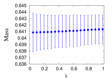
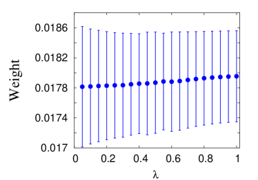
   Figure 1: Plot of ground-state pion mass, $m_{\pi}a$ (left) and spectral weight $w$ (right), versus global static weight, $\lambda$, for bare quark mass $ma=0.226$.

   

   

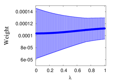
   Figure 2: Same as in Fig. 1 but for the nucleon for bare quark mass $ma=0.188$ ($m_{\pi}=583(3)\,{\rm MeV}$).

3. Local Dynamical Weight: For some quantities, such as for the ground-state mass and spectral weight of the pion displayed in Fig. 1, the dependence of the fitted results on the value of $\lambda$ is quite mild. For others, such as for the nucleon of Fig. 2, the dependence is stronger. Accordingly, we propose an adaptive procedure of absorbing any systematic error associated with the choice of $\eta$ into the statistical error, by upgrading each $\eta_{i}$ to a dynamical variable to be determined by the fit. It is incorporated as a dynamical fit variable by further augmenting the $\chi^{2}$:

   $$\chi_{\rm aug^{\prime}}^{2} = \chi^{2}+\chi_{\rm prior}^{2}+\chi_{\eta}^{2}$$ (15)

   $$\chi_{\rm prior}^{2} = \sum_{i}\frac{(\rho_{-}\tilde{\rho}_{i})^{2}}{\eta_{i}^{2}\tilde{\sigma}_{i}^{2}}$$ (16)

   $$\chi_{\eta}^{2} = \sum_{i}\frac{(\eta_{i}-\tilde{\eta_{i}})^{2}}{\tilde{\sigma}_{\eta}^{2}}$$ (17)

   The choice of $\tilde{\eta_{i}}$ and $\tilde{\sigma}_{\eta}$ is also somewhat arbitrary, and results in some uncertainty in assessing the systematic error; however, the dependence on these parameters is gentler than on the corresponding static global values and any remaining systematic error is masked by statistical error.

4. Global Dynamical Weight: In our fits presented here, we made the simplest choice of a special case of (c): we took all $\eta_{i}$ for different parameters to be the same global $\eta$, and took $\tilde{\eta}=1$ and $\tilde{\sigma}_{\eta}=1$.

   Often, the dependence of the results of the fit on the Global Static Weight is sufficiently smooth that the use of Global Dynamical Weight is unnecessary.

III.1.2 “Releasing the Constraint”

A way to mitigate the potentially aggressive nature of the fully-constrained fit in the Sequential Empirical Bayes Method is the following: When one is interested in estimating a particular parameter (i.e. the mass or weight of the ground state or $n^{\rm th}$ excited state) one takes the priors from the previous method and does a partially constrained fit: all other parameters are constrained except the one in question which is unconstrained (or perhaps only very lightly constrained). We say that the parameter to be estimated is “released” (from the constraint). The statistical error estimate obtained this way is larger and a more conservative choice. We will, by default, release the constraint for all of the final results presented.

III.1.3 “Scanning”

Referring back to our algorithm, if a prior is available, we use it as the value of the initial guess. But as a new parameter is introduced there is no prior, and an initial guess must be obtained by some other criterion. In practice, it may happen that different initial guesses lead to different values for the fit parameters, especially for the unconstrained fit. This may signal the presence of multiple local minima in the complicated $\chi^{2}$ topography. To address this we introduce and advocate the use of “scanning” over a grid of reasonable initial values and selecting that choice which leads to a descent to the lowest $\chi^{2}$. By extending the scan to a rather large region of parameter space, we ensure that the initial guesses for the parameters will not confine the $\chi^{2}$ minimization search to a single basin of local attraction, but rather will extend over many, including that of the global minimum.

III.2 Testing the Algorithm

III.2.1 “Reconstructing Artificial Data”

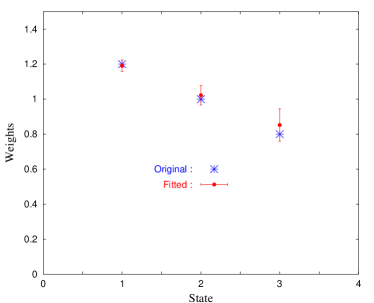
Figure 3: Recovery of parameters from artificially constructed data.

As there are a lot of ingredients to our modification of the standard constrained fit method (“Onion-Shell Data”, “Scanning”, “Global Dynamical Weight”, “Releasing the Constraint”) it is comforting to learn that the method can successfully reconstruct the parameters of artificially-constructed data where the true results are known independently of the fit. We created a sample of artificial data as a sum of five decaying exponentials, with means for masses and weights fixed at values close to those extracted from real data. Then, for simplicity, given this function, $G(t)$, we added an independent Gaussian noise at each value of $t$. When run through our fitting procedure, we were able to reconstruct the masses and weights for the ground state, first-excited state, and second-excited state (see Fig. 3); for these, the actual values were within one measured standard deviation of the measured masses.

III.2.2 “Partitioning the Configurations”

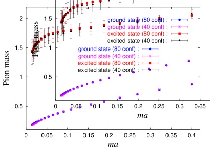
Figure 4: Test of partitioning the data. Ground and first excited state pion mass, $m_{\pi}a$, as a function of the bare quark mass $ma$.

We have constructed an automated and natural way of obtaining the priors from a subset of the data. However, one worries that there is a significant amount of “data snooping” which may make it difficult to estimate the systematic errors. (Strictly speaking, using any of the data to obtain the priors violates the Bayesian approach.) To alleviate these worries, we have implemented the following test: we partition the data into two non-intersecting sets of configurations, $A$ and $B$, with an equal number, $n_{A}=n_{B}=40$ of configurations in each set (which must still be large enough to permit stable covariant fits). Using the set $A$ of configurations, we perform our procedure outlined above of obtaining the priors gradually, from the ground state up, as the data set is monotonically enlarged by including earlier and earlier time slices. Now, regarding this entire procedure as a black box solely for the purposes of obtaining the priors, we next use this fixed set of priors in the canonical way Lepage et al. (2002) to perform a constrained fit separately on data set $B$ (for which there is no data snooping), on data set $A$ (maximal data snooping), and on the full set $A\cup B$ (partial data snooping but with greater statistics). Any disagreement beyond statistical errors can help assess systematic errors due to data snooping. In our case we found no appreciable differences beyond expected statistical fluctuations. Figure 4 shows a plot of the ground and first excited state pion mass, $m_{\pi}a$, as a function of the bare quark mass $ma$.

III.2.3 “Stability”

However priors are obtained, they can then be used in a standard constrained curve fitting procedure, wherein the fit window $t_{\rm min}$–$t_{\rm max}$ is held fixed (and as big as feasible), while the number of terms in the fit model is increased one-by-one until the fit results converge for the lowest few parameters of interest. To test whether the Sequential Empirical Bayes Method has produced reliable priors, we subsequently use its priors in the standard way Lepage et al. (2002); Morningstar (2002) as described above. Figure 5 illustrates the passing of this test.

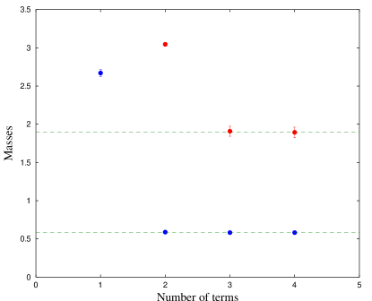
Figure 5: In a test of stability, priors had previously been selected by the Sequential Empirical Bayes Method. Now they are used in the standard constrained fit. The figure shows fit values for the lowest two masses from constrained fits (for all $t$’s) with different numbers of terms in the fit model. The data is from the pion two-point correlation function $\langle A_{4}A_{4}\rangle$ at bare quark mass $ma=0.188$ ($m_{\pi}=583(3)\,{\rm MeV}$).

III.2.4 “Fitting Errors”

Given the posterior probability distribution, $P(\rho|D)$, all statistics may be evaluated by computing integrals. In practice, such evaluation is often difficult to perform directly; Monte Carlo methods such as simulated annealing Fiebig (2002) can be used. Even so, the computational cost is often daunting and so approximations are sought. Most commonly, one may assume that the data set is sufficiently large that the Central Limit Theorem implies that $\chi^{2}_{\rm aug}$ is approximately quadratic about its minimum. We in fact use this approximation, and furthermore use the resulting fitting errors from a fit as the priors $\tilde{\sigma}$ for the next fit. To test this, we plot in Fig. 6 the $\chi^{2}_{\rm aug}$ as a function of $\rho$ in the neighborhood of the minimum. Superimposed is the parabola which is the quadratic approximation about the minimum. The two agree very well. Also calculated and plotted as ranges are the “fit error”, obtained from the quadratic approximation, and the second moment of the actual distribution. These too agree very well, and indicate that using the naive fit error as provided by the minimization routine is quite adequate.

Although fit errors are used to produce priors for the inner loops of the algorithm, all final errors reported are bootstrap errors.

Figure 6: Plot of the augmented $\chi^{2}_{\rm aug}$ in the vicinity of its minimum. It agrees well with a quadratic approximation, ensuring that the fit error provided by the minimization routine is adequate. The data is from the pion two-point correlation function at bare quark mass $ma=0.226$ ($m_{\pi}=633(10)\,{\rm MeV}$).

III.2.5 Caveat Emptor: Further Toy Model Results

It is crucial to be extremely conservative when making fits, especially when relying on Bayes’ inference methods. One must be sure to avoid announcing a “false positive”, that is making claim which cannot be guaranteed to be correct. We can understand in more detail how a false positive may emerge and how to design the procedure to avoid them, by testing variants of the SEB algorithm against a number of “toy models” where the actual values of the function’s parameters are known.

Suppose the artificial data is created with the three-state model function

$$G^{\rm true}(t) = w_{1}e^{-m_{1}t}+w_{2}e^{-m_{2}t}+w_{3}e^{-m_{3}t}$$

$$= w_{1}e^{-m_{1}t}\left(1+\frac{w_{2}}{w_{1}}e^{-(m_{2}-m_{1})t}+\frac{w_{3}}{w_{1}}e^{-(m_{3}-m_{1})t}\right),$$

and we want to perform a fit of the data sample generated by this function with fixed values of input parameters and Gaussian statistical error $\delta G(t)$ at each time slice $t$. Then SEB should work if the following holds:

1. There exists a $t_{1}$ such that in the time range $t_{1}<t<t_{\rm max}$,

   $$\frac{w_{2}}{w_{1}}e^{-(m_{2}-m_{1})t}<\delta G(t)\frac{1}{G(t)},$$ (19)

   so that in this range, the data can be fitted by $w_{1}e^{-m_{1}t}$. That is, there is a “plateau” in the effective mass plot for large time.

2. There exists a $t_{2}$ such that in the time range $t_{2}\leq t<t_{1}$,

   $$\frac{w_{3}}{w_{1}}e^{-(m_{3}-m_{1})t}<\delta G(t)\frac{1}{G(t)}<\frac{w_{2}}{w_{1}}e^{-(m_{2}-m_{1})t}$$ (20)

   so that in this range, the data can be well fitted by $w_{1}e^{-m_{1}t}+w_{2}e^{-m_{2}t}$.

3. In the time range $t<t_{2}$, the third state becomes important, and the full three-state model must be used in the fit.

Now the SEB is very adaptive; in the course of the iterative procedure, the ground state is fitted several times and allowed to float within a sigma or so of its current prior with each new fit. Thus the original criterion of the existence of a clear plateau need not be strictly enforced. But if the condition for the plateau is badly violated, or if the similar conditions for the excited states are badly violated, there is a possible danger of the algorithm gravitating toward a local minimum in the $\chi^{2}$ which is not the true value.

To illustrate, consider artificial data, constructed from the following three-state toy model

$$G(t;w_{i},m_{i}) = \sum_{i=1}^{3}w_{i}e^{-m_{i}t}$$

$$= 500e^{-0.85t}+400e^{-1.35t}+400e^{-1.75t}$$

in the time range $0\leq t\leq 15$, with relative errors (uncorrelated and Gaussian) increasing with time $t$ to mimic actual LGT data.

In keeping with the spirit of the SEB, we fit first to a single exponential over the time interval $t\in[t_{1},t_{\rm max}]$, then use the fitted ground state values as priors for a two-state partially-constrained fit in the time interval $t\in[t_{2},t_{\rm max}]$, and then use the fitted ground and first-excited state fit values as priors for a final three-state partially-constrained fit in the time interval $t\in[t_{\rm min},t_{\rm max}]$, where $t_{\min}=0\leq t_{2}\leq t_{1}\leq t_{\rm max}=15$. But to stress the caveat about the dangers of “false positives”, we explore all values for the pair $(t_{1},t_{2})$.

“Lowest Precision” case:

With statistical errors ranging from $\delta G/G\sim 0.011$ at $t=0$, to $\sim 0.12$ at $t=15$, the lowest $\chi^{2}/{\rm dof}$ fit is for $(t_{1},t_{2})=(10,7)$ with $m_{1}=0.855(7)$, $w_{1}=521(34)$, $m_{2}=3.10(62)$, $w_{2}=0.0004(1)$, $m_{3}=1.51(5)$, $w_{3}=769(35)$, that is, the fit fails to produce the input parameters of the toy model.

“Low Precision” case:

If the Gaussian noise is reduced by about a factor of two to $\delta G(t)/G(t)\sim 0.006$ at $t=0$, $\delta G(t)/G(t)\sim 0.05$ at $t=15$, then there are two solutions with the lowest $\chi^{2}/{\rm dof}=0.527$: a false positive with $(t_{1},t_{2})=(10,2)$ and $m_{1}=0.854(4)$, $w_{1}=518(23)$, $m_{2}=1.50(8)$, $w_{2}=701(63)$, $m_{3}=1.86(92)$, $w_{3}=69(62)$, and a fit which agrees with the input model: $(t_{1},t_{2})=(10,4)$ with $m_{1}=0.853(5)$, $w_{1}=511(29)$, $m_{2}=1.39(16)$, $w_{2}=369(188)$, $m_{3}=1.65(17)$, $w_{3}=408(188)$.

“High Precision” case:

If the Gaussian noise is further reduced to $\delta G(t)/G(t)\sim 0.001$ at $t=0$, $\delta G(t)/G(t)\sim 0.01$ at $t=15$ then the lowest $\chi^{2}/{\rm dof}=0.530$ does reproduce the input parameters: $(t_{1},t_{2})=(10,5)$, $m_{1}=0.851(1)$, $w_{1}=504(7)$, $m_{2}=1.38(6)$, $w_{2}=451(141)$, $m_{3}=1.77(10)$, $w_{3}=343(144)$.

Let $\Delta G(t)$ be the absolute value of the difference of the function $G^{\rm true}(t)$ of input parameters and the function $G^{\rm fitted}(t)$ of fitted parameters

$$\Delta G(t)=|G^{\rm true}(t)-G^{\rm fitted}(t)|.$$ (22)

A fit $G^{\rm fitted}(t)$ with reasonable small $\chi^{2}/{\rm dof}$ implies that the relation

$$\Delta G(t)<\delta G(t)$$ (23)

roughly holds at most times $t$. In other words, with this statistical error $\delta G(t)$, we cannot distinguish the fitted function $G^{\rm fitted}(t)$ from the original $G^{\rm true}(t)$.

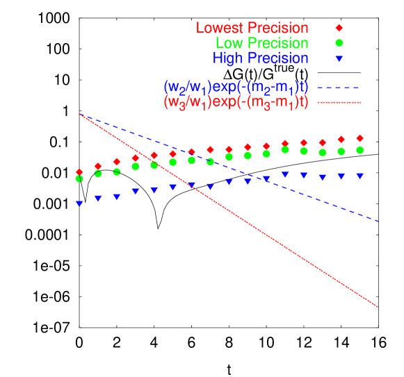
Figure 7: The relative errors of three data sets of increasing precision (“Lowest”, “Low”, and “High”) are plotted with points. The curved solid (black) curve is the plot of the function $\Delta G(t)/G^{\rm true}(t)$, which is the relative difference between original function $G^{\rm true}(t)=500\exp(-0.85t)+400\exp(-1.35t)+400\exp(-1.75t)$ and the false-positive fitted function $G^{\rm false}=521e^{-0.855t}+769e^{-1.51t}$ from the data set (“Lowest Precision”).

From Fig. 7 we see that the statistical errors of the data set (“Lowest Precision”) are all larger than the difference of the two functions in the full time range. This is the reason why the false positive can be chosen by the fit routine. The dashed (blue) straight line ($w_{2}/w_{1}\exp(-(m_{2}-m_{1})t)=0.8\exp(-0.5t)$) and the dotted (red) straight line ($w_{3}/w_{1}\exp(-(m_{3}-m_{1})t)=0.8\exp(-0.9t)$) intersect with the curve of relative errors at $t_{1}$ and $t_{2}$, respectively. This shows that the ground state dominates in the range $t\geq t_{1}$, the first-excited state plays a role in the range $t_{2}\leq t<t_{1}$, and the three states should all be included in the time range $t<t_{2}$. When the precision is higher, the statistical errors are smaller than the difference of two functions, in some time range, so that the fit can reject the false positive $G^{\rm false}(t)$.

Returning to the false positive of the “Lowest Precision” case, notice that when forced to fit to a three-state model, the fit prefers a two-state solution with the one weight essentially zero, and the remaining weight consistent with the sum of the true second and third weights and the remaining mass interpolating between the true masses. In short, the fit is content with averaging the two higher states into one. Also notice that it is the second weight which is zero. This is because, at the intermediate stage, a two-state model was forcing a fit to data completely dominated by a single state. Subsequently, as earlier times were added, the data could be described by two states, but since the would-be second state weight was by now constrained near zero, its role was supplanted by the third state in the model.

That is, by introducing the new (second) state into the model before the data was precise enough to discern it, spurious results were obtained. This suggests the cure: postpone the introduction of new states in the model until the data demands it (as evidenced by a sudden increase in the $\chi^{2}/{\rm dof}$).

In more detail, if the time range is large enough there exists a largest time $t_{1}$ beyond which the contamination of higher states will be obscured by the statistical errors and can be neglected so that in the time range $t\geq t_{1}$ the ground state dominates and the data can be well described by the single exponential $w_{1}\exp(-m_{1}t)$. Thus the time range $t\geq t_{1}$ is a good choice for the first step of SEB, and we can get a reasonably small $\chi^{2}/{\rm dof}$ over this ground-state effective-mass plateau. If we include more time slices with $t_{2}\leq t<t_{1}$, the contribution of the first excited state becomes significant, but the second excited state contributes little to the correlation function in this range. The presence of the first excited state results in a noticeable increase of the $\chi^{2}/{\rm dof}$ if we continue to force a single exponential as a fit model; the inclusion of one more term in the fit model is necessary. Continue this procedure until the time-slices are exhausted.

The Penultimate Algorithm: “Not-too-Soon”

1. The available data are in the time range $t_{min}-t_{max}$.

2. From effective mass plots, choose an initial time range $t\in[t_{\rm start},t_{\rm max}]$ to do an unconstrained one-mass fit. Use “scanning” – see Sect. III.1.3.

3. Include one more time slice and repeat an (independent) unconstrained one-mass fit, and monitor the fitted parameters ${m_{1},w_{1}}$ and the $\chi^{2}/{\rm dof}$.

4. If the fitted parameters and the $\chi^{2}/{\rm dof}$ do not change much, include one more time slice and repeat the previous step. This iteration stops if there is a noticeable change of $\chi^{2}/{\rm dof}$ and the values of the fitted parameters indicating a breakdown of the one-state model. Then set $t_{1}-1$ equal to the time at which the $\chi^{2}/{\rm dof}$ jumps, indicating the necessity of a two-mass fit for $t<t_{1}$. Set the priors for the ground state mass and weight equal to the fitted values from the last low–$\chi^{2}/{\rm dof}$ fit over $t\in[t_{1},t_{\rm max}]$.

5. Include one more mass term in the fit model and do a partially-constrained two-mass fit (with scanning) for $t\in[t_{1}-1,t_{\rm max}]$. The ground state priors are fixed at the values determined by the previous step. The first-excited state is unconstrained but scanned.

6. Repeat, adding time slices until the two-state model breaks down as indicated by a jump in the $\chi^{2}/{\rm dof}$. Then set $t_{2}-1$ equal to the time at which the $\chi^{2}/{\rm dof}$ jumps, indicating the necessity of a three-mass fit for $t<t_{2}$. Set the priors for the ground state and first-excited state mass and weight equal to the fitted values from the last low–$\chi^{2}/{\rm dof}$ fit over $t\in[t_{2},t_{\rm max}]$. Note that the ground-state priors are refreshed.

7. Repeat, adding more time slices and more fit-model terms (one at a time and only when necessary) and more until all time slices are used.

8. The highest state in the fit model will be absorbing all the contributions from higher states in the true function, and thus its fitted parameters will differ from the true values. Thus the highest state in the fit model must be rejected.

Now we return to the artificial data from the toy model “Lowest Precision”. Recall that when we assume a three-mass fit and independently try all pairs $(t_{1},t_{2})$, we obtained a false positive. But the statistical errors are so large that they obscure the contributions from excited states at all but the earliest time slices. Adding terms to the fit model prematurely led to spurious results. Now we apply the new method outlined immediately above to the same data.

A one-state fit works well for $t\in[t_{1},t_{\rm max}=15]$ until the $\chi^{2}$ suddenly jumps at the (proposed value of) $t_{1}=3$. Thus we set $t_{1}=4$. The values of the one-mass term fit over time range $[4,15]$ are used to set priors for $m_{1}$ and $w_{1}$, and a second term is added to the fit model. The two-term model works well for a fit in the range $[t_{2},15]$ with $t_{2}$ varying from 3 to 0. The two-mass model fit the data very well ($\chi^{2}/{\rm dof}=0.265$) in the whole time range with fitted parameters $m_{1}=0.855(7)$, $w_{1}=521(34)$, $m_{2}=1.51(5)$, $w_{2}=768(35)$. Since the two-mass fit exhausts all the time slices and does not show a noticeable increase of $\chi^{2}/{\rm dof}$, we don’t go ahead to include the third mass term in the fit model.

But this fit is a “false positive”! Since the statistical errors are larger than the difference between the false positive and the true solution (Eq. 23), the false positive cannot be rejected on the basis of its $\chi^{2}/{\rm dof}$, by this or any other method. So what have we gained? The difference this time is that this solution is exposed as a two-mass-term fit rather than a spurious three-term fit. And as always, the highest state in the fit must routinely be dropped since in general it can be contaminated by contributions from higher excited states.

We conclude that with the “Lowest Precision” data set, we cannot get an unambiguous estimate of the second and the third state. The fit is comfortable predicting the ground state parameters only (and they are correct). Thus the algorithm has not made a “false positive” claim.

Now, we illustrate this technique with another set of artificial data for which it will be possible to extract excited states. It will be instructive to monitor at the behavior of the $\chi^{2}/{\rm dof}$, but also to see how the fit parameters of each term in the fit model stabilize as time slices are added. Fig. 8 (left) plots the $\chi^{2}/{\rm dof}$ for data artificially constructed as a sum of four decaying exponentials. A one-term fit is adequate for time slice 13 ($t_{\rm max}=15$). But it is exposed as being entirely inadequate as time slice 12 is added to the data set to be fit. (The $\chi^{2}/{\rm dof}$ jumps tremendously because we have made the statistical errors on the data to be fit quite small, to illustrate the point.) So for time slices 6-12 a two-term fit model is used, and the fit is quite adequate. At time slice 5, however, the $\chi^{2}/{\rm dof}$ jumps tremendously, exposing the two-term fit as inadequate. Thus a third term is added at time slice 5. The three-term fit works down through time slice 2. At time slice 1, a fourth term must be added to keep the $\chi^{2}/{\rm dof}$ from being unreasonably large.

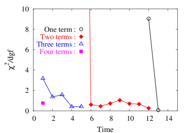
Figure 8: Behavior of the $\chi^{2}/{\rm dof}$ of the fit as earlier time slices are added to the fit range. A sudden jump indicates that the fit model is inadequate and that a new mass term should be added to the model. Accordingly, then the $\chi^{2}/{\rm dof}$ drops only to increase again as further time slices are added. “Not-too-Soon” addition of terms to the fit model prevents a single state being erroneously identified as two. Also shown are the behavior of the ground and first few excited states, which stabilize as more terms are added.

Meanwhile, Fig. 8 (right) monitors the masses of the lowest few states as more time slices are added to the data set and more terms are added (as necessary) to the fit model. At time slice 13, the one-term model is fitted with a ground-state mass (open circle). (Its value is consistent with the value obtained much later when time slices 1–12 have been added to the fit model and three more terms are added to the fit model. That is, time slices above 13 are sufficient to determine the ground-state mass, i.e the effective mass plot has “plateaued”. But more importantly for the efficacy of the algorithm, this fitted value remains stable later as the data and fit model are expanded.) At time slice 12, the second term is added to the fit model (solid diamonds). As each earlier time is added, the first-excited state mass changes by a sigma or so, as the augmented data is refit. This is important. It is saying that if a relatively small amount of data from time slices 12 and above suggested a somewhat inaccurate guess for the prior for this mass, then subsequent fits including data at time slices 8-11 can influence the value and bring it toward the correct value (at the horizontal line). By time slice 8, the first excited state mass has stabilized (at the correct value) and will not subsequently deviate through time slice 6. At time slice 5, the first-excited state mass deviates from the correct answer. But this is where the jump in the $\chi^{2}/{\rm dof}$ warns that the two-state fit model is inadequate; the first-excited state fitted mass is contaminated from higher states in the data. Adding a third term returns the fitted first-excited state mass to its correct value. It remains stably at this value with the addition of earlier time slices 2–4 to the three-state fit model (open triangles). Before the second-excited state has stabilized, we have run out of earlier time slices to add, and we can make no claim as to whether its fitted value is correct. (It isn’t.) But the algorithm has successfully fitted the first-excited state (and of course the ground state).

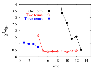
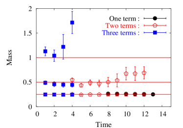
Figure 9: Same as in Fig. 8 but the artificial data is less precise (1%). Accordingly, the $\chi^{2}/{\rm dof}$ does not jump to such extreme values when the number of the terms in the fit model becomes inadequate.

Figs. 9 and 10 tell a similar story for artificial data which is less precise (1% and 5% respectively). The $\chi^{2}/{\rm dof}$ jump (indicating that another term should be added to the fit model) but, as one would expect, not as extremely as for the more precise data of Figs. 8.

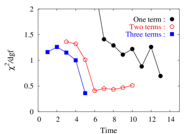
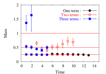
Figure 10: Same as in Fig. 8 but the artificial data is even less precise (5%).

III.2.6 Our Final Algorithm: “Just-in-Time”

As we saw in the last section, the “Not-too-Soon” algorithm avoids “false positives” by delaying the addition of a new term to the fit model before the data were able to discern it. However, there is the logical possibility of the opposite danger: if the new term is added too late, then there could potentially be an erroneous $n$-state fit of data which is in fact better described by $n+1$ states. If so, then the highest two states will be “averaged” into one. (So, for example, a fitted first excited state mass might take a value intermediate between the true first and second excited state masses.) The addition of further states to the fit model might then cover up this misidentification, and allow for this different kind of false positive.

One would think that an increased $\chi^{2}/{\rm dof}$ would warn of this danger; however, since the $\chi^{2}/{\rm dof}$ is an average over many time slices, it’s warning may come a time slice or two too late. If the data is such that a new term is discernible every couple of slices, then this may indeed lead to erroneous results.

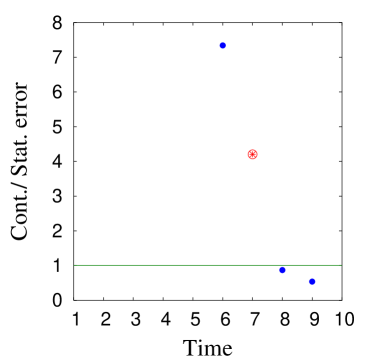
Figure 11: Ratio of the contribution to the fit model from a proposed new term, $w_{n}e^{-m_{n}t_{i}}$, compared to the statistical error $\delta G(t_{i}$) at the newest time slice $t_{i}$ added to the data set. The new term is deemed not needed at time slices $t_{i}=9$ and $t_{i}=8$. At time slice $t_{i}=7$, the ratio exceeds $1$ and the new term is conditionally accepted. The ratio remains above $1$ for time slice $t_{i}=6$ and below, confirming that the new term is needed. The data is from a fit of the Roper resonance at the same quark mass as in Fig. 14.

A final tweak of the algorithm addresses this issue: The “Just-in-Time” algorithm is the same as the “Not-too-Soon” algorithm outlined in the last section, except that the previous criterion for adding a new term to the fit model, namely that without this new term the $\chi^{2}/{\rm dof}$ would suddenly increase, is replaced by a more sensitive criterion: As a new time slice $t_{i}$ is added to the data set, a tentative fit is made with a proposed extra term, {$w_{n}$,$m_{n}$}. Then the contribution of this fitted term is compared to the statistical error at the new time slice

$$w_{n}e^{-m_{n}t_{i}}>\delta G(t_{i})$$ (24)

(See Fig. 11.) If Eq. 24 does not hold, then the new term is deemed not needed. If it does hold, then the new term is accepted (but only conditionally since the equation may hold only by statistical fluctuation). As new time slices are added, the new term must continue to pass this test. (This is stable: typically, if it passes the test once, it is likely to continue to pass the test at earlier time slices, since for these the relative error gets smaller and the fractional contribution gets larger.) If the test is failed before a higher-order term is conditionally added, then one returns to time slice $t_{i}$ and it is deemed that the $n$th term is not included in the fit. Then time $t_{i}-1$ is added to the data, a new proposal is made to add the $n$th term, and the process continues.

IV Some Physics Results

We have presented a list of algorithms with steadily increasing complexity but with steadily increasing robustness. The earliest and simplest “fixed $\Delta t$” algorithm, most easily described and presented first here as a template, was originally used (prematurely in retrospect) for some preliminary conference presentations. We now deem it too unsophisticated and do not use it anymore. The plain vanilla “variable $\Delta t$” algorithm is adequate provided that the level spacings are well separated and each term is saturated by several time slices. It is perfectly adequate to describe, for instance, the pion ground and excited state, as explained in Sect. IV.2. The plain “variable $\Delta t$” was used in the first version of our Roper paper and caused some erroneous results at high quark mass. This has been rectified by the use of the “Just-in-Time” algorithm for the updated version of our Roper paper and is briefly described in Sect. IV.3.

IV.1 The Simulation

On a $16^{3}\times 28$ lattice, we use the overlap fermion Neuberger (1998) and the Iwasaki gauge action Iwasaki (1985) with $\beta=2.264$. The lattice spacing, determined from the measured pion decay constant $f_{\pi}$, is determined to be $a=0.200(3)\,{\rm fm}$, and thus the lattice has spatial size of $3.2\,{\rm fm}$.

We adopt the following form for the massive Dirac operator Hernandez et al. (1999); Alexandrou et al. (2000); Capitani (2001)

$$D(m_{0})=(1-\frac{m_{0}a}{2\rho})\rho D(\rho)+m_{0}a,$$ (25)

where

$$D(\rho)=1+\gamma_{5}\epsilon(H),$$ (26)

so that

$$D(m_{0})=\rho+\frac{m_{0}a}{2}+(\rho-\frac{m_{0}a}{2})\gamma_{5}\epsilon(H),$$ (27)

where $\epsilon(H)=H/\sqrt{H^{2}}$ is the matrix sign function and $H$ is taken to be the hermitian Wilson-Dirac operator, i.e. $H=\gamma_{5}D_{w}$. Here $D_{w}$ is the usual Wilson fermion operator, except with a negative mass parameter $-\rho=1/2\kappa-4$ in which $\kappa_{c}<\kappa<0.25$. We take $\kappa=0.19$ in our calculation which corresponds to $\rho=1.368$. The massive overlap action is defined so that the tree-level renormalization of mass and wavefunction is unity.

We adopt the Zolatarev implementation van den Eshof et al. (2002a, b) of the optimal rational approximation Edwards et al. (1999); Dong et al. (2000) to approximate the matrix sign function. The inversion of the quark matrix involves nested do loops in this approximation. Further details of the procedure are given elsewhere Dong et al. (2002, 2000).

IV.2 Pion

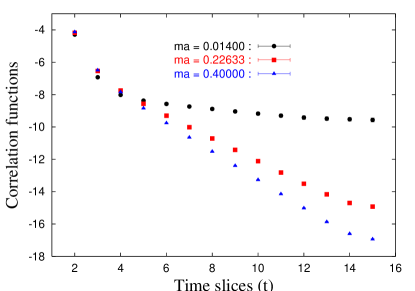
Figure 12: Two-point correlation function $\langle A_{4}A_{4}\rangle$ for the pion for three bare quark masses.

Figure 12 shows the correlation function for the correlator $\langle A_{4}A_{4}\rangle$. One can see that it is dominated by the ground state of the pseudoscalar channel (pion) over all but the few earliest time slices. This presents a problem for the default “fixed $\Delta t$” approach. Referring back to the algorithm of section II.3, we see that at each step of the algorithm, $\Delta t$ new time slices are added to the data while a new excited state is added to the fit model. Thus for the pion correlator, one would be trying to fit to a model with many states when the data is saturated by just the ground state. Forcing a fit may give misleading estimates of excited state parameters which are subsequently used as priors.

With the “variable $\Delta t$” refinement of the algorithm, rather than deciding a priori on the number of terms in the fit and adding time slices a fixed number at a time, one lets the data decide how many time slices to include with each enlargement of the data by choosing the minimum $\chi^{2}$ over a range of reasonable possibilities. Thus since the pion correlator is dominated by the ground state for many time slices, then many time slices will be automatically added before an attempt is made to fit the first-excited state.

In fact, we find that the “variable $\Delta t$” method works very well for the pion correlators. Figure 13 shows the results of the fit, the ground- and first-excited-state weight and mass as a function of the bare quark mass.

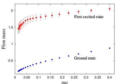
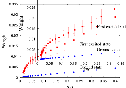
Figure 13: Ground and first-excited state pion mass $m_{\pi}a$, as a function of the bare quark mass $ma$ (left). Ground and first-excited stated pion weight, as a function of the bare quark mass $ma$ (right). Notice that the ground state weight does not diverge as the quark mass approaches zero for this $\langle A_{4}A_{4}\rangle$ correlator as it would for the $\langle PP\rangle$ correlator, where $P$ is the pseudoscalar density.

IV.3 The Roper Resonance

Studies using standard curve fitting have heretofore failed to satisfactorily identify the “Roper resonance” $N^{1/2+}(1440)$ of the nucleon on the lattice Lee and Leinweber (1999); Lee (2001); Lee et al. (2002); Richards et al. (2002); Sasaki et al. (2002a); Maynard and Richards (2002); Melnitchouk et al. (2003); Sasaki et al. (2002b); Sasaki (2003); Edwards et al. (2003). Our analysis is the first lattice calculation to obtain the masses of the Roper and $S_{11}(N^{1/2-}(1535))$ at low quark masses well in the chiral regime (with a pion mass as low as $180\,{\rm MeV}$). However, the effects of quenched artifacts, specifically the presence of ghost $\eta^{\prime}N$ states, complicates the physics as well as the functional form of fit model, and so the details of the calculation are presented elsewhere Dong et al. (2003a). To be sure, our calculation benefits from going to unprecedented low quark mass with the full chiral symmetry provided by overlap fermions, but the Sequential Empirical Bayes Method plays a crucial role.

It also presented a challenge and led to the refinement of the SEB from the “variable $\Delta t$” version to the “Just-in-Time” version. The first version of our Roper results Dong et al. (2003b) used the “variable $\Delta t$” method which, as we’ve seen, had until then been perfectly adequate to expose excited states (such as for the pion in Sec. IV.2) where the density of excited states is not too high. Compared to our final analysis with the “Just-in-Time” version Dong et al. (2003a), the results for the nucleon and $S_{11}$ did not change. The only change is for the Roper state at medium and heavy quark masses. Indeed our first results at medium-heavy masses passed the “Stability Plot” test (Fig. 14) and our focus returned to the more interesting light quark mass regime. Here the “variable $\Delta t$” criterion for when to add new states remains perfectly adequate for pion masses below $\sim 350\,{\rm MeV}$.

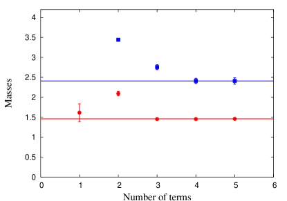
Figure 14: Stability test for the Roper resonance at bare quark mass $ma=0.268$ ($m_{\pi}=702(2)\,{\rm MeV}$). Priors had previously been selected by the plain “variable $\Delta t$” version of the Sequential Empirical Bayes Method. Now they are used in the standard constrained fit. The figure shows fit values for the lowest two masses (Nucleon and Roper) from constrained fits with different numbers of terms in the fit model. (At this mass, ghost states make no contribution, and so the fit model contains only exponentials.)

Subsequently, we came to realize that the “variable $\Delta t$” criterion that we adopted to introduce the excited state was not adequate for medium and heavy quarks, although it is adequate for the light quarks. In fitting someone else’s proprietary charmonium data, we realized that the crucial difference between the heavy quark spectrum and that of the light is that the ratio of the excited state mass to that of the ground state is much smaller in the heavy system, that is, the excitation spectrum in the heavy quark system is more dense. The earlier criterion erroneously resulted in obtaining the average of the higher excited states as the first excited state for the heavy system. In view of this, we devised the new and final “Just-in-Time” criterion (Sec. III.2.6), wherein a new term is added if its contribution is statistically significant at the current time slice. In fact, the penultimate “Not-too-Soon” algorithm (Sec. III.2.6), where the criterion for adding a new term to the fit model depends on a sudden jump in the $\chi^{2}/{\rm dof}$, works just as well as “Just-in-Time” for the Roper resonance at both medium-high and low quark masses. But for some charmonium data, or other test data constructed with a dense excited-state spectrum, “Just-in-Time” is somewhat better than “Not-to-Soon”, and because of its potential theoretical advantages is our method of choice.

Fig. 15 shows that our final algorithm passes the “Stability Test”. However, so did the earlier “variable $\Delta t$” algorithm. This and the fact that the extracted excited state mass changed alarmingly means that the “Stability Test” Lepage et al. (2002) is only a necessary but not a sufficient test for the reliability of constrained-curve fitting. We emphasize, however, that the source of the discrepancy has been identified and cured; the final algorithm can robustly protect against the averaging of excited states.

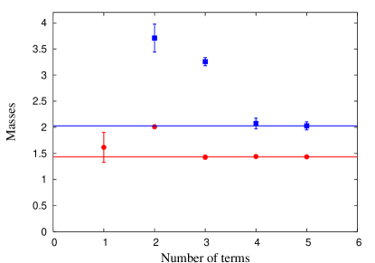
Figure 15: Same as for Fig. 14 but for our best and final “Just-in-Time” algorithm.

IV.4 Handling Ghost States

In the quenched approximation, there are artifacts associated with the absence of quark loops. One of the more interesting consequences is that the would-be $\eta^{\prime}$ propagator involves only double $\eta$ poles in “hairpin diagrams”. These lead to the chiral-log terms contributing to hadron masses; we see these clearly in our recent lattice calculation of pion and nucleon masses Dong et al. (2003c). Another quenched artifact is the contribution of ghost states in the hadron propagators as first seen in the $a_{0}$ meson channel Bardeen et al. (2001) where the ghost $S$-wave $\eta^{\prime}\pi$ state lies lower in mass than the $a_{0}$ (for sufficiently small quark mass). We have seen a similar effect in analysis of the excited nucleon spectrum where a $P$-wave $\eta^{\prime}N$ lies close in mass to the Roper resonance Dong et al. (2003a), and its presence must be carefully disentangled by the fitting code. More dramatically, in the negative-parity channel $S_{11}$ ($N^{\frac{1}{2}-}$), the lowest $S$-wave $\eta^{\prime}N$ state has a mass lower than that of the $S_{11}$ for small quark mass. Since the $\eta$–$\eta$ coupling in the hairpin diagram is negative Bardeen et al. (2001), the $S_{11}$ correlator changes sign with increasing time separation Dong et al. (2003a). This effect is only seen at small enough quark masses, and thus is not seen in most lattice simulations at much higher masses.

As a result, the form of the fitting function changes; there are extra non-exponential terms. Nevertheless, the SEB can successfully handle this situation. It is crucial to enforce the physical constraint that the weight of the ghost state be negative; otherwise there would be no way to distinguish it from the physical state (e.g. Roper) lying nearby. The details of the fitting model and the results of the fitting (using the “Just-in-Time” SEB algorithm) for the Roper and $S_{11}$ are in Dong et al. (2003a).

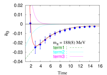
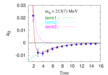
Figure 16: $a_{0}$ correlators for our lowest quark mass for which $m_{\pi}=188(8)\,{\rm MeV}$ (left) and $m_{\pi}=213(7)\,{\rm MeV}$ (right). The negative dip of the correlators is an indication of the domination of the ghost $S$-wave $\eta^{\prime}\pi$ state over the physical $a_{0}$. The curves are contributions to the fit model and are explained in the text.

Another example is displayed in Fig. 16 where we show the $a_{0}$ propagator at two low quark masses, for which $m_{\pi}=188(8)\,{\rm MeV}$ (left) and $m_{\pi}=213(7)\,{\rm MeV}$ (right). The most dramatic feature of the data in each figure is the negative dip of the correlator at time slice 3 and above. The solid (red) line passing through the data is the result of the SEB fit. The two dominant contributions to the fit model are negative and are indicated by the dashed (green) line labeled “term 1” and by the solid (cyan) curve labeled “term 2”. They are modeled by the expression

$$w_{1}(1+E_{\pi}t)e^{-m_{\eta^{\prime}\pi}t}$$ (28)

where $w_{1}$ is constrained to be negative and the $(1+E_{\pi}t)$ factor reflects the double-pole nature of the hairpin diagram Dong et al. (2003a). We fit $m_{\eta^{\prime}\pi}$, the mass of the interacting would-be $\eta^{\prime}$ and $\pi$ state. Since we work in a finite box, the $\eta^{\prime}\pi$ states are discrete and they are constrained to be near the energy of the two non-interacting particles, each with $E=\sqrt{m^{2}+\sum_{i}(\frac{2}{a}\sin\left(\frac{p_{i}}{2})\right)^{2}}$ for discrete lattice momentum $p_{i}=\frac{2\pi n}{L}$ where $n$ is an integer. For “term 1”, $n=0$ and for “term 2”, $n=1$. The contribution of the physical state $a_{0}$ is positive and is indicated by dotted magenta curve in each figure. In summary, our SEB algorithm is quite capable of handling non-standard forms of the fit model including negative-normed ghost-state contributions and can fit successfully the data.

V Summary

We have advocated refinements of Bayesian-inspired constrained-curve fitting which we believe better stabilizes fits at low quark mass. This permits analysis where the values of fit parameters are not reliably known a priori, such that their use as priors might be dangerously biased.

In the “Sequential Empirical Bayes Method”, we have constructed an automated and natural way of reliably obtaining the priors from naturally-nested subsets of the data (“onion shells”). For the prototype described here, a time-dependent two-point correlation function $G(t)$, we first obtain estimates of the ground state mass and weight from unconstrained fits to a subset of data restricted to large times. These are then used as the priors in a subsequent constrained fit. A sequence of (fully or partially) constrained fits follow. At each step, more data from adjacent earlier times are added and another term is added to the fit model. When a new parameter is added, its first estimate is obtained from a fit in which it is unconstrained but previously introduced parameters are constrained. After each fit, the fitted values of each parameter are used as the priors for the next fit. Thus the value of each prior is free to float from one fit to the next, and thus is not prevented from changing significantly over the course of the several steps of the iteration as more and more data are added. This mitigates any bias which may have been introduced wherein the first estimates of a prior are inaccurate due to statistical fluctuations in the smaller initial data set. In the final step, as the last data are added, no new terms are added to the fit model. A final fit for each parameter leaves it unconstrained (or very weakly constrained) with all other parameters constrained by priors set equal to the latest fitted values. Our final bootstrapped errors obtained from “releasing the constraint” in this way are larger than for a completely-constrained fit and are selected as a conservative estimate.

We have found some further refinements to be fruitful: (a) We use a “scanning” technique to automate the selection of an initial value for a new parameter for its first unconstrained fit. We thus avoid the pitfall of the $\chi^{2}$ minimization routine becoming trapped in the attraction basin of a local, but not global minimum. (b) The weight factor (essentially a Lagrange multiplier), $\lambda$, balances the influence of the data versus the priors in determining the output of a fit. Decreasing $\lambda$ from its canonical Bayesian value of 1, can be used to assess the systematic error associated with the choice of prior(s). We advocate absorbing this systematic error into a statistical error by promoting $\lambda$ to be “global dynamical weight”, that is, a fit parameter with its own prior mean and standard deviation.

We have tested that our algorithm can successful recover the correct fit parameters of an artificial data set, constructed as a sum of decaying exponentials with realistic values of the parameters. For one channel (corresponding to using only the local-local two-point correlation function), the masses and weights of the ground and first-excited states are fit to within a measured standard deviation of the true values. Thus, for our real data, we restrict ourselves to measuring only the lowest two states, even though we use four or five states in the fit model. This is sufficient for our present purposes.

Our method is not in strict accord with the Bayesian philosophy, as we use subsets of the data to guide the selection of the priors. Nevertheless, the following mitigates bias from such data snooping: (a) The data is naturally nested in that a subset of data restricted to large times can provide a fair estimate of the lowest state parameters. Adiabatically increasing the data set with the introduction of new terms in the fit model gives fair estimates of excited-state parameters to be used as priors. (b) The priors are given ample opportunity to change in accordance with the data in the several steps of the algorithm. Is this enough? To test this we “partition the data” by configuration into equally-sized but disjoint sets and apply our algorithm to one half to obtain priors and then use these priors in a standard constrained fit on the other half (in strict accord with the Bayesian philosophy) and on the full data set. We see no difference beyond expected statistical errors; that is, no bias is seen.

In further studies using artificially constructed data with known means and errors (“toy models”) we have presented some caveats against the careless application of the algorithm which might result in a state being spuriously identified as a combination of two, leading to a “false positive” prediction. These false positives were avoided in the toy model studies by insisting that a new term be added to the fit model “Just-in-Time”, that is only after a fit with fewer terms is deemed inadequate.

For this pilot study, we have analyzed the ground and first-excited masses and weights for the pion from overlap fermions on a quenched $16^{3}\times 28$ lattice with spatial size $La=3.2\,{\rm fm}$ and pion mass as low as $180\,{\rm MeV}$, commented on the history of the use and suitability of variations of the SEB algorithm for extracting the Roper resonance Dong et al. (2003a), and given another example ($a_{0}$) where the method can handle ghost states.

- (1)
- Lepage et al. (2002) G. P. Lepage et al., Nucl. Phys. Proc. Suppl. 106, 12 (2002), eprint [http://arXiv.org/abs]hep-lat/0110175.
- Morningstar (2002) C. Morningstar, Nucl. Phys. Proc. Suppl. 109, 185 (2002), eprint [http://arXiv.org/abs]hep-lat/0112023.
- Asakawa et al. (2001) M. Asakawa, T. Hatsuda, and Y. Nakahara, Prog. Part. Nucl. Phys. 46, 459 (2001), eprint hep-lat/0011040.
- Nakahara et al. (1999) Y. Nakahara, M. Asakawa, and T. Hatsuda, Phys. Rev. D60, 091503 (1999), eprint hep-lat/9905034.
- Fiebig (2002) H. R. Fiebig, Phys. Rev. D65, 094512 (2002), eprint hep-lat/0204004.
- Dong et al. (2003a) S. J. Dong et al. (2003a), eprint hep-ph/0306199.
- Robert (2001) C. P. Robert, The Bayesian Choice (Springer, New York, 2001).
- Press (2003) S. J. Press, Subjective and Objective Bayesian Statistics (Wiley, Hoboken, 2003).
- Robbins (1950) H. Robbins, Proc. Second Berkeley Symposium Math. Stat. and Prob. , 131 (1950).
- Robbins (1955) H. Robbins, Proc. Third Berkeley Symposium Math. Stat. and Prob. 1, 157 (1955).
- Robbins (1964) H. Robbins, Ann. Math. Stat. 35, 1 (1964).
- Press et al. (1992) W. Press et al., Numerical Recipes in C, The Art of Scientific Computing, Second Edition (Cambridge University Press, Cambridge, 1992).
- Neuberger (1998) H. Neuberger, Phys. Lett. B417, 141 (1998), eprint [http://arXiv.org/abs]hep-lat/9707022.
- Iwasaki (1985) Y. Iwasaki, Nucl. Phys. B258, 141 (1985).
- Hernandez et al. (1999) P. Hernandez, K. Jansen, and L. Lellouch, Phys. Lett. B469, 198 (1999), eprint hep-lat/9907022.
- Alexandrou et al. (2000) C. Alexandrou, E. Follana, H. Panagopoulos, and E. Vicari (2000), eprint hep-lat/0009004.
- Capitani (2001) S. Capitani, Nucl. Phys. B592, 183 (2001), eprint [http://arXiv.org/abs]hep-lat/0005008.
- van den Eshof et al. (2002a) J. van den Eshof, A. Frommer, T. Lippert, K. Schilling, and H. A. van der Vorst, Nucl. Phys. Proc. Suppl. 106, 1070 (2002a), eprint hep-lat/0110198.
- van den Eshof et al. (2002b) J. van den Eshof, A. Frommer, T. Lippert, K. Schilling, and H. A. van der Vorst, Comput. Phys. Commun. 146, 203 (2002b), eprint hep-lat/0202025.
- Edwards et al. (1999) R. G. Edwards, U. M. Heller, and R. Narayanan, Phys. Rev. D59, 094510 (1999), eprint hep-lat/9811030.
- Dong et al. (2000) S. J. Dong, F. X. Lee, K. F. Liu, and J. B. Zhang, Phys. Rev. Lett. 85, 5051 (2000), eprint hep-lat/0006004.
- Dong et al. (2002) S. J. Dong et al., Phys. Rev. D65, 054507 (2002), eprint hep-lat/0108020.
- Lee and Leinweber (1999) F. X. Lee and D. B. Leinweber, Nucl. Phys. Proc. Suppl. 73, 258 (1999), eprint hep-lat/9809095.
- Lee (2001) F. X. Lee (LHPC), Nucl. Phys. Proc. Suppl. 94, 251 (2001), eprint hep-lat/0011060.
- Lee et al. (2002) F. X. Lee, D. B. Leinweber, L. Zhou, J. M. Zanotti, and S. Choe, Nucl. Phys. Proc. Suppl. 106, 248 (2002), eprint hep-lat/0110164.
- Richards et al. (2002) D. G. Richards et al. (LHPC), Nucl. Phys. Proc. Suppl. 109A, 89 (2002), eprint hep-lat/0112031.
- Sasaki et al. (2002a) S. Sasaki, T. Blum, and S. Ohta, Phys. Rev. D65, 074503 (2002a), eprint hep-lat/0102010.
- Maynard and Richards (2002) C. M. Maynard and D. G. Richards (UKQCD) (2002), eprint hep-lat/0209165.
- Melnitchouk et al. (2003) W. Melnitchouk et al., Phys. Rev. D67, 114506 (2003), eprint hep-lat/0202022.
- Sasaki et al. (2002b) S. Sasaki, K. Sasaki, T. Hatsuda, and M. Asakawa (2002b), eprint hep-lat/0209059.
- Sasaki (2003) S. Sasaki, Prog. Theor. Phys. Suppl. 151, 143 (2003), eprint nucl-th/0305014.
- Edwards et al. (2003) R. G. Edwards, U. M. Heller, and D. G. Richards (LHP), Nucl. Phys. Proc. Suppl. 119, 305 (2003), eprint hep-lat/0303004.
- Dong et al. (2003b) S. J. Dong et al. (2003b), eprint hep-ph/0306199,v1.
- Dong et al. (2003c) S. J. Dong et al. (2003c), eprint hep-lat/0304005.
- Bardeen et al. (2001) W. Bardeen, A. Duncan, E. Eichten, N. Isgur, and H. Thacker (2001), eprint [http://arXiv.org/abs]hep-lat/0106008.