QCD String formation and the Casimir Energy

Abstract

Three distinct scales are identified in the excitation spectrum of the gluon field around a static quark-antiquark pair as the color source separation R is varied. The spectrum, with string-like excitations on the largest length scales of 2–3 fm, provides clues in its rich fine structure for developing an effective bosonic string description. New results are reported from the three–dimensional Z(2) and SU(2) gauge models, providing further insight into the mechanism of bosonic string formation. The precocious onset of string–like behavior in the Casimir energy of the static quark-antiquark ground state is observed below R=1 fm where most of the string eigenmodes do not exist and the few stable excitations above the ground state are displaced. We find no firm theoretical foundation for the widely held view of discovering string formation from high precision ground state properties below the 1 fm scale.

1 QCD String Spectrum and the Casimir Energy

Last year, we presented a new analysis of the fine structure in the QCD string spectrum at the Lattice 2002 conference. Shortly afterwards, two papers were submitted using complementary methods for finding definitive signals of bosonic string formation from the rich excitation spectrum[1] and the ground state Casimir energy.[2]

QCD String Spectrum

Three exact quantum numbers which are based on the symmetries of the problem determine the classification scheme of the gluon excitation spectrum in the presence of a static $q\bar{q}$ pair.[1]

Figure 1: Short distance degeneracies which are not string-like and their crossover towards the QCD string spectrum are shown from Ref. 1 where further details are explained. The color coded solid curves with simulation points, which identify energy levels degenerate in the asymptotic string limit, are only shown for visualization and do not represent fits to the data. The yellow line without data points marks a lower bound for the onset of mixing effects with glueball states which requires careful interpretation. The symbol LW indicates the ${\rm R}$ range of high precision Casimir energy calculations from Ref. 2.

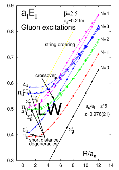
We adopt the standard notation from the physics of diatomic molecules and use $\Lambda$ to denote the magnitude of the eigenvalue of the projection ${\bf J}_{g}\!\cdot\hat{\bf R}$ of the total angular momentum ${\bf J}_{g}$ of the gluon field onto the molecular axis with unit vector $\hat{\bf R}$. The capital Greek letters $\Sigma,\Pi,\Delta,\Phi,\dots$ are used to indicate states with $\Lambda=0,1,2,3,\dots$, respectively. The combined operations of charge conjugation and spatial inversion about the midpoint between the quark and the antiquark is also a symmetry and its eigenvalue is denoted by $\eta_{CP}$. States with $\eta_{CP}=1(-1)$ are denoted by the subscripts $g(u)$. There is an additional label for the $\Sigma$ states; $\Sigma$ states which are even (odd) under a reflection in a plane containing the molecular axis are denoted by a superscript $+$ $(-)$. Hence, the low-lying levels are labeled $\Sigma_{g}^{+}$, $\Sigma_{g}^{-}$, $\Sigma_{u}^{+}$, $\Sigma_{u}^{-}$, $\Pi_{g}$, $\Pi_{u}$, $\Delta_{g}$, $\Delta_{u}$, and so on, $\Sigma_{g}^{+}$ designating the ground state. For convenience, we use $\Gamma$ to denote these labels in general. For better resolution of the fine structure in the spectrum, the gluon excitation energies ${\rm E_{\Gamma}(R)}$ were extracted from Monte Carlo estimates of generalized large Wilson loops on lattices with small ${\rm a_{t}/a_{s}}$ aspect ratios and improved action. Restricted to the R=0.2–3 fm range of a selected simulation, the energy spectrum is shown in Fig. 1 for 10 excited states.

On the shortest length scale, the excitations are consistent with short distance physics without string–like level ordering in the spectrum. A crossover region below 2 fm is identified with a dramatic rearrangement of the short distance level ordering. On the largest length scale of 2–3 fm, the spectrum exhibits string-like excitations with asymptotic ${\rm\pi/R}$ string gaps which are split and slightly distorted by a fine structure. It is remarkable that the torelon spectrum of a closed string, with one unit of winding number around a compactified direction, exhibits a similar fine structure on the 2–3 fm scale, as reported for the first time at Lattice 2003.[3] This finding eliminates the boundary effects of fixed color charges as the main source of the fine structure in the distorted spectrum.

Casimir Energy

In a complementary study,[2] a string–like Casimir energy and the related effective conformal charge, ${\rm C_{eff}(R)=-12R^{3}F^{\prime}(R)/(\pi(D-2))}$, were isolated where ${\rm F(R)}$ is the force between the static color sources and D is the space-time dimension of the gauge theory with bosonic string formation. With unparalleled accuracy, ${\rm C_{eff}(R)}$ was determined for the gauge group SU(3) in D=3,4 dimensions, in the range ${\rm 0.2~{}fm<R<1.0~{}fm}$, below the crossover region of the string spectrum. A sudden change with increasing R, well below 1 fm, was observed in ${\rm C_{eff}(R)}$, breaking away from the the short distance running Coulomb law towards the string-like ${\rm C_{eff}(R)\approx 1}$ behavior. This was interpreted as a signal for early bosonic string formation. The results are surprising because the scale $\rm R$ is not large compared with the expected width of the confining flux, and more quantitatively, the string-like Casimir energy behavior is observed in the ${\rm R}$ range where the spectrum exhibits complex non-string level ordering, as shown in Fig. 1. We will try to develop now a better understanding of the seemingly paradoxical situation.

2 Bosonic String Formation in the Z(2) Gauge Model

The three-dimensional Z(2) lattice gauge model represents considerable simplification in comparison with four-dimensional lattice QCD. The SU(3) group elements on links are replaced by Z(2) variables, and the reduction to three dimensions implies a nontrivial continuum limit with a finite fixed point gauge coupling.

Dual $\phi^{4}$ Field Theory Representation

The main features are easily seen from the dual transformation of the Z(2) gauge model to Ising variables which can be replaced by the real scalar field of ${\rm\phi^{4}}$ field theory in the critical region. The continuum model exhibits confinement and bosonic string formation in the broken phase of the Ising representation. In addition, a nontrivial glueball spectrum is observed[5] with finite masses when measured in units of the string tension. The string tension of the confining flux in the Z(2) gauge model becomes the interface energy in the dual Ising-$\phi^{4}$ representation, and the lowest mass ${\rm 0^{+}}$ glueball state of the gauge theory with mass m maps into the elementary scalar of the dual lattice, with inverse correlation length m in the critical region. Higher glueball states are Bethe-Salpeter bound states of the elementary scalar.[5] The dual $\phi^{4}$ Lagrangian of the Z(2) gauge model, in rigorous theoretical setting, is in analogy with the dual Landau-Ginzburg superconductivity model which attempts to describe the unknown microscopic quark confinement mechanism of QCD.

The Ising-${\rm\phi^{4}}$ field theory model is particularly intriguing from the microscopic string theory viewpoint, if we recall Polyakov’s work on the connection with the theory of random surfaces. Using loop equations of closed Wilson loops near the continuum limit, he conjectured the equivalence of the three-dimensional Z(2) lattice gauge theory to a fermionic string theory.[7]

Renormalization Scheme

In three euclidean dimensions, the Z(2) model is described in the critical region (continuum limit) by a real order parameter field $\phi$ with the Lagrangian

$${\mathcal{L}}={\rm-\frac{1}{2}(\partial_{\mu}\phi_{0})^{2}-\frac{g_{0}}{4!}(\phi_{0}^{2}-\frac{3m_{0}^{2}}{g_{0}})^{2}}~{}.$$ (1)

The most frequently used renormalization scheme requires in the broken phase that the tadpole diagrams completely cancel without coupling constant renormalization ($g=g_{0}$) and with wave function renormalization $\phi_{0}=\sqrt{Z}\phi$. In the following, with lattice cutoff, we define a scheme with finite coupling constant renormalization keeping the renormalized mass of the elementary scalar exactly at the pole of its propagator. Since the wave function renormalization is finite to every order, for convenience we choose Z=1 in 1-loop calculations. With ${\rm g_{0}=g+\delta g}$, ${\rm v^{2}_{0}\equiv 3m^{2}_{0}/g_{0}=v^{2}+\delta v^{2}}$, the renormalized Lagrangian for elementary excitations $\eta$ around the vacuum expectation value $\phi=v$ is the starting point of the renormalized loop expansion with two counterterms to one-loop order,

$$\delta{\rm v^{2}}={\rm lim_{V\rightarrow\infty}\;\;\frac{3}{2}g\cdot\frac{1}{V}}\sum_{\vec{\rm k}}\frac{1}{E^{0}_{\vec{\rm k}}}~{},~{}~{}~{}~{}\delta{\rm g=\frac{g^{2}}{m}\;\frac{ln3}{32\pi}}~{}.$$ (2)

The infinite spatial volume limit is taken in the sum over the spectrum of inverse lattice energies of free massive excitations $E^{0}_{\vec{\rm k}}$ with periodic boundary conditions. The coupling constant counterterm ${\rm\delta g}$ satisfies the renormalization condition on the physical propagator pole to one-loop order.

In the presence of a pair of static sources, represented by a Wilson loop in the Z(2) gauge model, the renormalization procedure is unchanged in the Ising-${\rm\phi^{4}}$ field theory description. The only change is in the lattice Lagrangian where the sign of the nearest neighbor interaction term is flipped on links which puncture the surface of the Wilson loop on the dual Z(2) gauge lattice. This flip represents a disorder line, or seam, between the two static sources on the spatial lattice. The end points of the seam are fixed but otherwise it is deformable by a “gauge transformation” of variables without changing the partition function. This invariance is inherited from the gauge invariant representation of the Wilson surface in the Z(2) gauge model.

Numerical Implementation of the Loop Expansion The dual transformation of the Z(2) model to Ising variables facilitates very efficient simulations with multispin coding. The loop expansion provides theoretical insight into Monte Carlo simulations of the excitation spectrum using high statistics multispin Ising codes complemented by ${\rm\phi^{4}}$ field theory codes. Since the fixed point value ${\rm u^{*}}$ of the dimensionless coupling constant ${\rm u=g/m}$ is not small, the simulations provide an important cross-check on the convergence of the loop expansion which itself has to be implemented in a numerical procedure. The renormalized loop expansion in the presence of static sources requires the following three steps.

(i) First, for a given physical mass m and renormalized coupling g, the time independent renormalized classical field equation,

$${\rm-\frac{\partial^{2}\phi_{s}(x,y)}{\partial x^{2}}-\frac{\partial^{2}\phi_{s}(x,y)}{\partial y^{2}}-\frac{1}{2}m^{2}\phi_{s}(x,y)+\frac{g}{6}\phi^{3}_{s}(x,y)=0~{},}$$ (3)

of the static soliton $\phi_{s}$ is solved on the lattice in the $\vec{\rm r}={\rm(x,y)}$ plane with flipped nearest neighbor interaction links along the seam between static sources. In the Z(2) gauge model, the two sources can be interpreted as opposite sign charges with an electric flux connecting them. In the ${\phi^{4}}$ representation we refer to the $\phi_{s}$ classical solution as a static soliton, rather than the earthy flux–tube term. In the numerical procedure, a generalized Newton type nonlinear iterative scheme was implemented to obtain $\phi_{s}$ to double precision accuracy.

(ii) Second, the fluctuation spectrum around the static soliton ${\rm\phi_{s}(x,y)}$ is determined by splitting the field into the classical solution plus fluctuations, ${\rm\phi(x,y,t)=\phi_{s}(x,y)}$ + ${\rm\eta(x,y,t)}$, with the eigenmodes of the fluctuation field ${\rm\eta(x,y,t)=\sum_{n}[a_{n}(t)\psi_{n}(x,y)+a^{\dagger}_{n}(t)\psi^{*}_{n}(x,y)]}$ satisfying the eigenvalue equation

$${\rm-\frac{\partial^{2}\psi_{n}}{\partial x^{2}}-\frac{\partial^{2}\psi_{n}}{\partial y^{2}}+U^{\prime\prime}(\phi_{s})\psi_{n}=E^{2}_{n}\cdot\psi_{n}~{}.}$$ (4)

The time dependence of the fluctuation field $\eta$ is given in interaction picture by ${\rm a_{n}(t)=a_{n}(0)e^{-iE_{n}t}}$ where the Hamiltonian is split into a quadratic part and an interaction part of the $\psi_{n}$ eigenmodes. The second derivative of the ${\rm U(\phi)=\frac{g}{4!}(\phi^{2}-\frac{3m^{2}}{g})^{2}}$ renormalized field potential energy is taken with respect to $\phi$ in Eq. (4), with $\phi=\phi_{s}$ substituted subsequently. Two parity quantum numbers ${\rm P_{x},~{}P_{y}}$ split the eigenmodes into four separate symmetry classes. With the two sources located at ${\rm(x,y)=(R/2,0)}$ and ${\rm(x,y)=(-R/2,0)}$, the quantum number ${\rm P_{x}=\pm 1}$ corresponds to the reflection symmetry ${\rm x\rightarrow-x}$ of ${\rm\psi_{n}(x,y)}$ and ${\rm P_{y}=\pm 1}$ corresponds to the ${\rm y\rightarrow-y}$ reflection symmetry. The full spectrum of eigenvalues and eigenfunctions of Eq. (4) are computed by an Arnoldi diagonalization procedure in the finite volume of the lattice. Using the parity symmetries of the theory, diagonalization of large lattices with sizes up to 200x200 in the (x,y) plane were performed.

(iii) Third, the systematic renormalized loop expansion with the $\phi_{s}$ static soliton background is developed by building the finite volume field propagator ${\rm D_{F}(}\vec{\rm r}{\rm,t;}\vec{\rm r}{\rm\,{}^{\prime},t^{\prime})}$ in Minkowski time,

$${\rm D_{F}(}\vec{\rm r}{\rm,t;}\vec{\rm r}{\rm\,{}^{\prime},t^{\prime})})=\sum_{n}{\rm i\int\frac{dp_{0}}{2\pi}}\frac{\psi_{n}(\vec{\rm r})\psi^{*}_{n}(\vec{\rm r}\,^{\prime})}{{\rm p^{2}_{0}-E_{n}^{2}+i\epsilon}}{\rm e^{-ip_{0}(t-t^{\prime})}}~{},$$ (5)

from the static $\psi_{n}(\vec{\rm r})$ eigenmodes. An euclidean rotation is performed on the propagator during the numerical evaluation of the loop diagrams. The counterterms ${\rm\delta v^{2}}$ and ${\rm\delta g}$ are used to remove loop divergences in the continuum limit and to keep the exact pole location at the physical mass m. Using the propagator of Eq. (5), the fluctuation correction to the static soliton profile $\phi_{s}$ was calculated to one-loop order, together with similar calculations of the ground state energy and excitation energies. In this work, we only report numerical results on the fluctuation spectrum of Eq. (4) and its 1-loop contribution to the ground state energy.

String Excitations in the Loop Expansion

For sufficiently large R, the discrete ${\rm P_{y}=-1}$ bound state spectrum of Eq. (4) is expected to evolve into the asymptotic ${\rm E_{N}=\pi N/R}$ ${\rm(N=1,2,\ldots})$ Dirichlet string spectrum of massless string excitations which originate from the translational mode of the well-known one-dimensional $\phi^{4}$ soliton by the following simple consideration.

Consider first the spatial lattice in the finite (x,y) plane with a seam of flipped links winding around the compact x–direction with periodic boundary condition. The classical solution ${\rm\phi_{tor}(y)=m\sqrt{3/g}\;tanh(m|y|/2)}$ of Eq. (3) defines the torelon which is independent of x and winds around the compact x–direction with a seam positioned at y=0. We use continuum notation for the torelon and its excitations, but finite cutoff and volume effects are included in the numerical work. For ${\rm x>0}$, the transverse profile of the torelon is identical to that of the well-known one-dimensional soliton, and for ${\rm x<0}$ a sign flip is involved because of the seam at y=0. The torelon eigenmodes of Eq.(4) with ${\rm P_{y}=-1}$ have the simple form

$${\rm\psi^{tor}_{{}_{N}}(x,y)=\sqrt{\frac{g}{2m^{3}}}\;\phi_{tor}^{\prime}(y)\cdot\sqrt{1/R}\;e^{ip_{{}_{N}}\cdot x}},$$ (6)

with quantized momenta, ${\rm p_{{}_{N}}=2\pi N/R,~{}N=\pm 1,\pm 2,\ldots}$, running along x in the compact interval R with periodic boundary condition. The energy spectrum is given by ${\rm E_{N}=2\pi N/R}$, with positive N values.

The classical transverse profile ${\rm\phi_{tor}(y)}$ of the torelon coincides, to a good approximation, with that of the static soliton $\phi_{s}$, if the separation between the sources is large enough. The static soliton profile $\phi_{s}$ does not interpolate from -v at large negative y to +v for large positive y at fixed x because of the flipped links along the seam. Rather, $\phi_{s}$ approaches v everywhere, far away from the seam line. The eigenmodes of the fluctuation operator are restricted now between the two sources and they are close to the form

$${\rm\psi^{static}_{{}_{N}}(x,y)=\sqrt{\frac{g}{2m^{3}}}\;\phi_{tor}^{\prime}(y)\cdot\sqrt{2/R}\;sin(\pi N/x)},~{}-R/2\leqq x\leqq R/2~{},$$ (7)

with N taking positive integer values. The spectrum of these standing waves is the same as that of a massless Dirichlet string oscillating in the (x,y) plane with fixed ends. The excited eigenmodes of the effective Schrödinger equation, like the one of Fig. 2b for N=8, are therefore in one-to-one correspondence with massless Dirichlet string oscillations. The spectrum and the wave functions are expected to be somewhat distorted at finite R because of the distortions of the effective Schrödinger potential around the sources.

Representative examples of the numerical work are shown in Fig. 2 where the static soliton solution ${\rm\phi_{s}(x,y)}$ on a 160x80 spatial lattice in the (x,y) plane corresponds to source separation R=100 and physical mass m=0.319 in the critical region (all dimensional quantities are expressed in lattice spacing units). For later comparisons, the lattice correlation length ${\rm m^{-1}}$ and the renormalized coupling g were chosen in the critical region to match one of our Monte Carlo simulations with v=0.45 and string tension ${\rm\sigma=0.0101}$.

Figure 2: The static soliton solution $\phi_{s}$ of field equation (3) is shown in (a) with the choice R=100 and renormalized parameters given in the text; (b) shows the N=8 massless string excitation of the static soliton from the numerical diagonalization of the eigenvaule equation (4); the second massive string excitation (K=2 breathing mode) is shown in (c) from the numerical solution of the eigenvalue equation, and compared in (d) to exact Monte Carlo simulation of the same state with remarkable agreement.

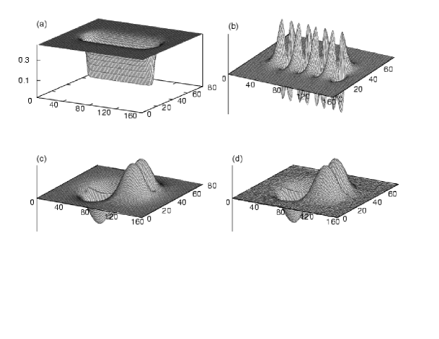
The static soliton solution $\phi_{s}(\vec{\rm r})$ determines the attractive potential energy of the effective Schrödinger eigenvalue problem in Eq. (4) which has a discrete bound state spectrum and a nearly continuous dense spectrum above the glueball threshold m representing scattering states on the static soliton in the infinite lattice volume limit.

The one–dimensional soliton, with classical mass ${\rm 2m^{3}/g}$, has a massive intrinsic excitation, or breathing mode, whose excitation energy is ${\rm(\sqrt{3}/2)m}$. In the large R limit, the intrinsic excitations of $\phi_{s}$ with ${\rm P_{y}=+1}$ become massive breathing modes of the Dirichlet string. The asymptotic spectrum of a massive string, given by ${\rm E_{K}=\sqrt{3m^{2}/4+\pi^{2}K^{2}/R^{2}},~{}K=1,2,\ldots}$, is associated with eigenmodes like the K=2 wave function of Fig. 2c. The corresponding standing wave solutions,

$${\rm\psi_{{}_{K}}(x,y)=\sqrt{3m/4}\;sech(my/2)\;tanh(m|y|/2)\cdot\sqrt{2/R}\;sin(\pi K/x)}~{},$$ (8)

originate from the massive excitations of the torelon with restriction to standing waves in the ${\rm-R/2\leqq x\leqq R/2}$ interval.

3 Probing the String Theory Limit

We describe the $\eta(\vec{\rm r},{\rm t})$ fluctuations around the static soliton $\phi_{s}$ by the sum of three fields, $\eta(\vec{\rm r},{\rm t})=\xi(\vec{r},t)+\chi(\vec{r},t)+\varphi(\vec{r},t)$, with

$${\rm\xi(x,y,t)} = {\rm\sum_{N}[a_{N}(t)\psi_{N}(x,y)+a^{\dagger}_{N}(t)\psi^{*}_{N}(x,y)]}~{},$$

$${\rm\chi(x,y,t)} = {\rm\sum_{K}[a_{K}(t)\psi_{K}(x,y)+a^{\dagger}_{K}(t)\psi^{*}_{K}(x,y)]}~{},$$

$${\rm\varphi(x,y,t)} = {\rm\sum_{n}[a_{n}(t)\psi_{n}(x,y)+a^{\dagger}_{n}(t)\psi^{*}_{n}(x,y)]}~{},$$

where $\xi$ is restricted to bound states with negative ${\rm P_{y}}$ parity which are expected to evolve into massless string excitations for large R. The field $\chi$ is restricted to ${\rm P_{y}=+1}$ parity bound states which evolve into massive string excitations, and $\varphi$ is a sum over scattering states above the ${\rm 0^{+}}$ glueball threshold m in the continuum.

These fields are coupled in the interaction Lagrangian, and when the massive fields $\chi$ and $\varphi$ are integrated out, we get a nonlocal Lagrangian in the ${\rm\xi(x,y,t)}$ field describing massless string excitations in the large R limit. As indicated by Eq. (7), the y–dependence in all the ${\rm P_{y}=-1}$ parity bound state wave functions is approximately factored out in the large R limit. Hence, the ${\rm\xi(x,y,t)}$ field can be replaced on large length scales by the field ${\rm f(x,t)}$ which becomes the geometric string variable of low energy excitations measuring the displacements of the flux center–line in the y–direction as a function of x and t.

Effective String Action

The nonrenormalizable effective action of the ${\rm f(x,t)}$ field, with the massive fields integrated out, is given in a derivative expansion by

$${\rm S_{eff}(f)} = -\int{\rm dxdt\bigg{[}\frac{1}{2\pi\alpha^{\prime}}\;\left(1-\frac{1}{2}(\partial f)^{2}-\frac{1}{8}((\partial f)^{2})^{2}-\frac{1}{16}((\partial f)^{2})^{3}+\cdots\right)}$$ (9)

$${}+{\rm const\cdot(\partial f)^{2}\Box(\partial f)^{2}+\cdots\bigg{]}}\;,$$

where $\partial\sim m^{-1}$ is a long wavelength expansion. The string tension $\sigma$ can be expressed as ${\rm\sigma=(2\pi\alpha^{\prime})^{-1}}$, and the notation ${\rm(\partial f)^{2}=\partial_{\mu}f\partial^{\mu}f}$ is used in Eq. (9). Since $f$ is related to massless Goldstone excitations, originating from the restoration of translation invariance in torelon quantization, only derivatives of f appear in ${\rm S_{eff}}$. The first three terms in the derivative expansion come from the kinetic terms in the original $\phi^{4}$ field theory action. They are independent of the details of the field potential except for the overall factor of ${\rm(2\pi\alpha^{\prime})^{-1}}$. The first line in Eq. (9) agrees with the equivalent terms of the Nambu-Goto (NG) action, ${\rm S_{NG}={\rm(2\pi\alpha^{\prime})^{-1}}\sqrt{1-(\partial f)^{2}}}$, when expanded in ${\rm(\partial f)^{2}}$. The second line in Eq. (9) has contributions from the geometric curvature, but new contributions also appear whose geometric origin remains unclear. This is where the effective string action begins to show deviations from the NG string. To correct for end effects around the static sources, the effective action of Eq. (9) has to be augmented by boundary operators for the complete description of the Dirichlet string.

Exact Excitation Spectrum from Simulations

First, the physical mass, the vacuum expectation value v, and the renormalized coupling g were determined in high precision Monte Carlo simulations of the bulk euclidean lattice action in the Ising-${\rm\phi^{4}}$ field theory representation without the seam of flipped links. The renormalized physical parameters were used as input to compare the loop expansion with simulations in the presence of static sources. The excitation spectrum around the static sources was determined from Monte Carlo estimates of correlation matrices which included an extended set of optimized operators. These operators were built from eigenfunctions of the fluctuation operator on two-dimensional time slices of the lattice.

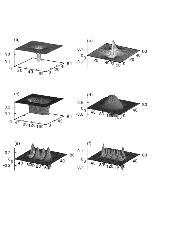
Simulation results are shown in Fig. 3 for string formation as R is stretched. The shape of the static soliton profile ${\rm\phi_{s}(x,y)}$ around the sources is depicted in the (x,y) plane of the two-dimensional spatial lattice for R=10 and R=100. With the scale set by the string tension, the two R values correspond to 0.3 fm and 3 fm, respectively. The renormalized bulk physical parameters of the simulations were given in the discussion of Fig. 2 as m=0.319, v=0.45, and ${\rm\sigma=0.0101}$. At the smaller R value, the static soliton with bag–like shape is not stretched, and there is only one bound state excitation below the glueball threshold. At R=3 fm, the stretched static soliton supports many string excitations, with the N=1,4,8 wave functions displayed. The Monte Carlo simulations are in good agreement with results from the eigenmodes of the fluctuation operator. This is indicated by the good match of Fig. 2a versus Fig. 3c and Fig. 2b versus Fig. 3f.

Figure 3: The soliton profile for R=10 is shown in (a), with the only bound state wave function below the glueball threshold depicted in (b). At R=100, the stretched soliton configuration shown in (c) exhibits several string-like excitation with the N=1 wave function shown in (d), N=4 in (e), and N=8 in (f). The simulation results match the loop expansion of Fig. 2 with common renormalized parameters.

Figure 4: The energy gap ${\rm\Delta E}$ above the ground state is plotted as ${\rm\Delta E/(N\pi/R)-1}$ to show percentage deviations from the asymptotic ${\rm N=1}$ string level. Several Z(2) simulations with cyan, blue, red, and green points are combined with good scaling properties. The open circles represent D=3 SU(2) results after readjusting the ratio of the string tension $\sigma$ to the glueball mass in Z(2). The null line coresponds to the tree level ${\rm\pi/N}$ NG string gaps. The dashed blue and green lines are 1–loop and two–loop NG approximations, repectively, and the black line is the full NG prediction.

Matching the Excitation Spectrum to the String Action

A large number of excitation spectra were obtained from highly accurate simulations as R was varied in a wide range from 0.3 fm to approximately 10 fm. A good test for string formation is provided by the behavior of the spectrum as a function of R. The NG spectrum,

$${\rm E_{N}=\sigma R\left(1-\frac{D-2}{12\sigma R^{2}}\pi+\ \frac{2\pi N}{\sigma R^{2}}\right)^{\frac{1}{2}}}~{},$$ (10)

with fixed end boundary conditions in D dimensions, was calculated in Ref. arvis. N=0 corresponds to the string ground state and positive integer N values label the excitations of the Dirichlet string. Although there exists an inconsistency in the quantization of angular momentum rotations around the ${\rm q\bar{q}}$-axis at finite ${\rm R}$ values unless ${\rm D=26}$, the problem asymptotically disappears in the ${\rm R\rightarrow\infty}$ limit.[8] This is expected from the earlier discussion on string formation in the loop expansion. Indeed, derived in a consistent D=3 $\phi^{4}$ field theory, the first few terms of the effective string action match the coefficients of their NG counterparts as seen in Eq. (9). If a string limit is reached for a large enough R range, the expansion of ${\rm E_{N}}$ into inverse powers of R from Eq. (9) should agree with the simulations at least to one nontrivial order. At small R values the expansion will break down since the mathematical NG string will be the inconsistent description of the bag-like soliton and its excitations in three dimensions.

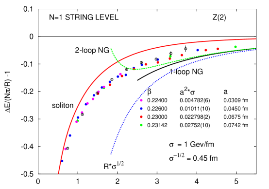
The comparison of simulations to string theory is illustrated in Fig. 4 where the exact N=1 excitation is plotted against the numerical spectrum of the fluctuation operator and the predictions of the Nambu-Goto string model. The numerical spectrum from Eq. (4) is the renormalized tree level starting point of the loop expansion in ${\rm\phi^{4}}$ field theory setting without assuming string formation. It is close in shape and details to the exact results for the entire R range, as shown by the solid red line with the soliton tag in Fig. 4. It is expected that higher loop corrections will bring the agreement even closer. The simulations, however, deviate substantially from the predictions of the loop expansion in the NG string model, particularly at smaller ${\rm R}$ values below 1 fm where the loop expansion suddenly begins to diverge. The string formation for large R is clearly seen in the spectrum of Fig. 4 and all the other spectra we obtained, but further work is needed for quantitative matching of the coefficients in the effective string action.

Our results differ from the findings of Ref. CHP where simulations of the finite temperature Z(2) string were reported in good agreement with the expansion of the NG model to 1–loop order below the R=1 fm scale.

4 The Casimir Energy Puzzle

The breakdown of the effective string description below 1 fm and the related Casimir energy paradox are illustrated with the calculation of the ground state energy from the renormalized fluctuation operator around the static $\phi_{s}$ soliton. In the renormalized loop expansion, the early onset of the string-like ${\rm C_{eff}(R)\approx 1}$ behavior in the R range below 1 fm is not associated with massless string eigenmodes which are mostly missing for ${\rm R\lesssim 1}$ fm. The results are consistent with the direct simulations of ${\rm C_{eff}(R)}$ and the spectrum in our Z(2) model. The simulations of Refs. JKM,LW1 present the same puzzle in QCD. If there is any physics associated with this puzzle, it remains unresolved.

Casimir Energy from the Fluctuation Operator The soliton ground state energy ${\rm E_{s}}$ in Eq. (11),

$${\rm E_{s}} = {\rm E^{cl}_{s}+\frac{1}{2}\sum_{\alpha}E_{\alpha}-\frac{1}{2}}\sum_{\vec{k}}{\rm E}_{\vec{k}}^{0}$$ (11)

$$- {\rm\frac{g}{12}\delta v^{2}\int\left[\phi_{s}-\frac{3m^{2}}{g}\right]dxdy+\frac{\delta g}{4}\int\left[\phi_{s}-\frac{3m^{2}}{g}\right]^{2}dxdy~{},}$$

includes the renormalized classical energy ${\rm E^{cl}_{s}}$, the sum of zero point energies summed over all eigenmodes $\alpha$ of the fluctuation operator of Eq. (4), and a sum over all momenta ${\vec{k}}$ in the zero point energy of the bulk vacuum without sources.

Figure 5: The red points are from high precision Ising-$\phi^{4}$ simulations. The solid black curve with NG label is the full NG prediction, ${\rm C_{eff}(R)=1}$ is the asymptotic string result which corresponds to the tree-level NG prediction. The dashed green line shows the 1-loop approximation which includes the first correction to tree level from the ${\rm R^{-1}}$ expansion of Eq. (10). The solid red line is calculated from the numerical evaluation of Eq. (11). The dashed blue line is obtained from the full red line by subtracting the ${\rm E^{cl}_{s}}$ contribution.

Figure 6: The ground state fluctuation energy density is plotted for R=40. The two peaks represent large fluctuation contributions around the static sources.

The difference of the two eigenmode sums is still divergent in the continuum limit. The ${\rm\delta v^{2}}$ counterterm removes this divergence and contributes a finite $\vec{r}$-dependent energy density to the ground state. The ${\rm\delta g}$ counterterm also contributes a finite and $\vec{r}$-dependent ground state energy density.

Exact Ground State Results

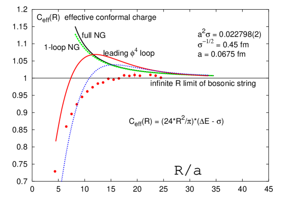
The simple definition ${\rm C_{eff}(R)=-24R^{2}(E_{s}^{\prime}(R)-\sigma)/(\pi(D-2))}$ was used to isolate the effective Casimir energy term in the ground state of the soliton. The first derivative ${\rm E_{s}^{\prime}}$ was directly simulated on the lattice by a special method we developed. The string tension $\sigma$ was determined in high precision separate runs from the ground state of long torelons. The simulations in Fig. 5 are also compared with the predictions of the Nambu-Goto (NG) string model and the predictions of Eq. (11) from the numerical evaluation of the fluctuation operator spectrum.

The agreement of ${\rm C_{eff}(R)}$ with exact simulation results, as determined from the fluctuation operator spectrum, is quite good down to very small R values. At smaller R values, full agreement can only be expected from higher loop corrections. It is interesting that the classical contribution of $\phi_{s}$ to ${\rm C_{eff}(R)}$ is significant below 1 fm. At large R, in the true string formation limit, the higher loop corrections should not contribute to the asymptotic 1/R Casimir term.

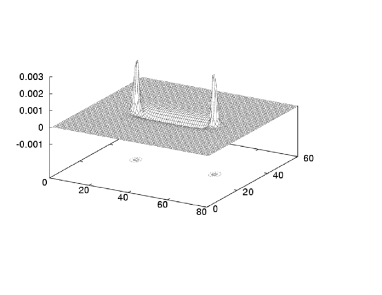
The dominant contribution to the ground state energy of the static soliton from the fluctuation operator is coming from the continuum spectrum but the ground state energy density remains concentrated around the static soliton. This is also seen in the Casimir energy density which is calculated from the first derivative of the energy density with respect to R, integrating to ${\rm C_{eff}(R)}$ as we explicitly checked. For illustration, the Casimir energy density is shown in Fig. 6.

Although the 1/R expansion of ${\rm C_{eff}(R)}$ from the NG prediction of Eq. (10) is not divergent below 1 fm, it breaks away from the data in a rather dramatic fashion.

5 Conclusions

We established bosonic string formation in a large class of gauge theory models from a direct study of the excitation spectrum at large separation of the static sources. The spectrum, with string-like excitations on the length scales of 2–3 fm and beyond, provides clues in its rich fine structure for developing an effective bosonic string description. The matching of the string-like spectrum to an effective string action remains a challenge.

Our results at small R differ from the findings of Ref. CHP where simulations of the finite temperature Z(2) string were reported in good agreement with the expansion of the NG model to 1–loop order below the R=1 fm scale. This agreement was interpreted as further support at finite temperature for the precocious onset of bosonic string formation in QCD below the 1 fm scale as reported in Ref. LW1.

We find no firm theoretical foundation for discovering string formation from high precision ground state properties below the 1 fm scale. The explanation for string–like finite temperature free energy behavior below 1 fm also remains unclear. Further work is needed to understand the interpretation of the results from Refs. LW1,CHP which present impressive high precision simulations.

References

- [1] K.J. Juge, J. Kuti, and C. Morningstar, Phys. Rev. Lett. 90, 161601 (2003).
- [2] M. Lüscher and P. Weisz, JHEP 0207, 049 (2002).
- [3] K.J. Juge, J. Kuti, F. Maresca, C. Morningstar, and M. Peardon, hep-lat/0309180, Proceedings of Lattice 2003, July 15-19, Tsukuba, Japan.
- [4] M. Caselle, M. Hasenbusch, M. Panero, JHEP 0301, 057 (2003).
- [5] M. Caselle, M. Hasenbusch, P. Provero, K. Zarembo, Nucl.Phys. B623, 474 (2002).
- [6] M. Baker, hep-ph/0301032, talk given at the 5th International Conference on Quark Confinement and the Hadron Spectrum, Gargnano, Italy, September 2002.
- [7] A.M. Polyakov, Phys. Lett. 82B, 247 (1979); 103B, 211 (1981).
- [8] J. F. Arvis, Phys. Lett. 127B, 106 (1983).