Abstract

We present the results of an extensive lattice calculation of the renormalization constants of bilinear and four-quark operators for the non-perturbatively ${\cal O}(a)$-improved Wilson action. The results are obtained in the quenched approximation at four values of the lattice coupling by using the non-perturbative RI/MOM renormalization method. Several sources of systematic uncertainties, including discretization errors and final volume effects, are examined. The contribution of the Goldstone pole, which in some cases may affect the extrapolation of the renormalization constants to the chiral limit, is non-perturbatively subtracted. The scale independent renormalization constants of bilinear quark operators have been also computed by using the lattice chiral Ward identities approach and compared with those obtained with the RI-MOM method. For those renormalization constants the non-perturbative estimates of which have been already presented in the literature we find an agreement which is typically at the level of 1%.

PACS numbers: 11.15.Ha, 12.38.Gc, 11.10.Gh.

1 Introduction

The increasing availability of computing resources has allowed a reduction of the statistical errors in current lattice QCD calculations at the level of few percent or less. The corresponding systematic uncertainties, however, are significantly larger, in some cases even by one order of magnitude. For this reason, a major effort in lattice calculations is aimed to reduce and to better control the various sources of systematic uncertainties. An important ingredient, in this respect, is the use of non-perturbative renormalization (NPR) techniques. By avoiding the perturbative expansion in the determination of the renormalization constants (RCs), these techniques remove the uncertainty associated with the truncation of the perturbative series and allow to reduce the systematic error involved in the renormalization procedure of the lattice matrix elements at a level of accuracy which is comparable or better than the present statistical one.

The first NPR technique was proposed almost 20 years ago. Within this approach the RCs are determined by requiring that the renormalized lattice Green functions satisfy the proper chiral Ward identities (WIs) [1]. This theoretically nice and numerically accurate approach suffers, however, of an important limitation: the use of chiral WIs only permits the determination of scale independent RCs (and mixing coefficients). After [1], it took about 10 years before other two NPR methods, which can be used in principle to compute any RC, were developed. They are based on the so called ${\rm RI/MOM}$ [2] and Schrödinger Functional (SF) schemes [3]. In the ${\rm RI/MOM}$ scheme the renormalization conditions are imposed, non-perturbatively, on quark and gluon Green functions at large external momenta, while in the SF approach they are imposed on Green functions computed in a small volume. More recently, a new proposal for NPR has been suggested in [4], and it is based on the study of lattice correlation functions at short distance in $x$-space. The results of the first numerical investigations of this approach have been presented in [5, 6].

The non-perturbative ${\rm RI/MOM}$ renormalization method has been already largely applied in lattice calculations to determine the RCs of several classes of operators for different versions of the lattice action (see for example refs. [8]-[13]). In this paper we present the results of an extensive ${\rm RI/MOM}$ calculation of the RCs of the complete set of bilinear and four-fermion $\Delta F=2$ and $\Delta I=3/2$ operators, for the non-perturbatively ${\cal O}(a)$-improved Wilson action [14] in the quenched approximation. The results are obtained at four values of the lattice coupling, in the range $6.0\leq\beta\leq 6.45$. Particular attention in the present calculation has been dedicated to the evaluation and control of systematic uncertainties:

• Discretization errors have been evaluated by studying the behaviour of the RCs as a function of the lattice coupling, $g(a)$, and of the renormalization scale. In the case of bilinear quark operators, since the action and the operators are non-perturbatively improved at ${\cal O}(a)$, leading discretization effects are of ${\cal O}(a^{2})$. These effects have been further reduced to ${\cal O}(g^{4}a^{2})$ by using the results of a recent perturbative calculation of the relevant correlation functions [15]. On the other hand, the four fermion operators considered in this study are not improved, and we are left in this case with leading discretization effects of ${\cal O}(a)$.

• Finite volume effects have been examined by comparing the results of two independent simulations performed, at the same value of the lattice coupling ($\beta=6.0$), on different lattice volumes.

• Goldstone pole contributions: power suppressed contributions coming from the Goldstone pole, which may affect the extrapolation to the chiral limit of the RCs of the pseudoscalar density and of the four-fermion operators coupled to the Goldstone boson, have been non-perturbatively subtracted.

The scale independent RCs of the vector and axial-vector currents, $Z_{V}$ and $Z_{A}$, and the ratio $Z_{P}/Z_{S}$, have also been determined in this study by using the lattice chiral WI approach, and the results are compared with those obtained with the ${\rm RI/MOM}$ method. We also compare our determinations of these constants with those obtained by the ALPHA [16, 17] and LANL [18] Collaborations by using the WI method, and our determination of $Z_{P}$ with the one obtained by ALPHA [19] within the SF approach. We find an agreement which is typically at the level of 1%. Since the systematics involved in these approaches are different, these comparisons provide additional confidence on the high level of accuracy reached in the implementation of the ${\rm RI/MOM}$ non-perturbative method.

Our final results for the RCs of bilinear quark operators and four-fermion operators are collected in tables 2-7. Preliminary results of the present study have been presented at the Lattice 2002 conference [5, 20].

The plan of this paper is as follows. In sec. 2 we give the details of the numerical simulation and briefly review the non-perturbative ${\rm RI/MOM}$ method used to determine lattice RCs. The various sources of systematic errors involved in the calculation are discussed in sec. 3, where we also provide estimates of the corresponding uncertainties. The results for the RCs of bilinear quark operators obtained with the ${\rm RI/MOM}$ method are summarized in sec. 4. In this section, we also compare these results with those obtained by using the WI method, with predictions of one-loop boosted perturbation theory and with the results of refs. [16]-[19]. The ${\rm RI/MOM}$ determination of the RCs of the four-fermion $\Delta F=2$ operators is discussed in sec. 5 and we end the paper by presenting our conclusions. More technical issues concerning the ${\cal O}(a)$-improvement of the RCs and the Goldstone pole contributions to the Green functions of four-fermion operators are collected in appendix A and B respectively.

2 Details of the lattice calculation

The lattice parameters used in this study are summarized in table 1.

lj $\beta=6/g_{0}^{2}$	6.0	6.0	6.2	6.4	6.45
lj $c_{SW}$	1.769	1.769	1.614	1.526	1.509
lj $L^{3}\times T$	$16^{3}\times 52$	$24^{3}\times 64$	$24^{3}\times 64$	$32^{3}\times 70$	$32^{3}\times 70$
lj $\#\ {\rm conf.}$	500	340	200	150	100
lj $a^{-1}(GeV)$	2.00(10)	2.00(10)	2.75(14)	3.63(18)	3.87(19)
lj $\kappa_{1}$	0.1335	0.13300	0.1339	0.1347	0.1349
lj $\kappa_{2}$	0.1338	0.13376	0.1344	0.1349	0.1351
lj $\kappa_{3}$	0.1340	0.13449	0.1349	0.1351	0.1352
lj $\kappa_{4}$	0.1342	——	0.1352	0.1353	0.1353
lj $\kappa_{cr}$	0.135225(5)	0.135217(7)	0.135815(3)	0.135747(2)	0.135686(2)

Table 1: Summary of the lattice details and parameters used in this work. We also give the values of the inverse lattice spacing and of the critical hopping parameter ($\kappa_{cr}$).

We have generated ${\cal O}(1000)$ gauge configurations in the quenched approximation, by using the non-perturbatively ${\cal O}(a)$-improved Wilson action. The improvement coefficient $c_{SW}$ has been determined in ref. [14], as a function of the coupling constant. We have considered four different values of the lattice coupling, namely $\beta=6.0$, $6.2$, $6.4$ and $6.45$, corresponding to inverse lattice spacings varying approximately between 2 and 4 GeV. The estimates of the inverse lattice spacing given in table 1, and used in the numerical analysis, have been determined from the study of the static quark anti-quark potential [21] by setting the scale $r_{0}=0.530(25)$ fm, which corresponds to $a^{-1}(\beta=6)=2.0(1)\,{\rm GeV}$. The uncertainty takes into account the typical spread of the results obtained in the determination of the lattice spacing in the quenched theory. We emphasize that mainly ratios of scales, rather than their absolute values, are relevant for the present calculation and for these ratios the static quark anti-quark potential provides an accurate determination.

For each value of the coupling, the RCs have been computed at four values of the light-quark mass and eventually extrapolated to the chiral limit. The values of the Wilson hopping parameter used in the simulations are listed in table 1, together with the corresponding critical values determined from the vanishing of the axial WI mass. The Wilson parameters correspond to bare quark masses which, in lattice units, are in the range $0.01\leq a\,m_{q}\leq 0.05$. The same set of gauge configurations and quark propagators used in this study have been also used in ref. [22], where additional details on the simulation can be found. In order to study finite volume effects we have considered two independent lattice simulations at $\beta=6.0$, performed on different lattice sizes. The main purpose of the simulation on the larger volume was the study of $K\to\pi\pi$ decays [23, 24] and this motivates the different choice of the values of quark masses.

The non-perturbative determination of the RCs with the ${\rm RI/MOM}$ method is based on the numerical evaluation, in momentum space, of correlation functions of the relevant operators between external quark and/or gluon states. In the case of the bilinear quark operators $O_{\Gamma}={\overline{q}}\Gamma q$, where $\Gamma=S,P,V,A,T$ stands respectively for $I,\gamma_{5},\gamma_{\mu},\gamma_{\mu}\gamma_{5},\sigma_{\mu\nu}$, the relevant Green function is

$${G}_{\Gamma}(p,p^{\prime})=\int d^{4}x\,d^{4}y\,e^{-ip\cdot x+ip^{\prime}\cdot y}\,\langle\widehat{q}(x)O_{\Gamma}(0)\widehat{\overline{q}}(y)\rangle\,,$$ (1)

where $\widehat{q}$ and $\widehat{\overline{q}}$ are renormalized quark fields. By using ${G}_{\Gamma}(p,p^{\prime})$ and the renormalized quark propagator,

$$\widehat{S}(p)=\int d^{4}x\,e^{-ip\cdot x}\,\langle\widehat{q}(x)\widehat{\overline{q}}(0)\rangle\,,$$ (2)

one evaluates the forward amputated Green function

$$\Lambda_{\Gamma}(p)=\widehat{S}(p)^{-1}{G}_{\Gamma}(p,p)\widehat{S}(p)^{-1}\,.$$ (3)

The ${\rm RI/MOM}$ renormalization method consists in imposing that the forward amputated Green function, computed in the chiral limit in a fixed gauge and at a given (large) scale $p^{2}=\mu^{2}$, is equal to its tree-level value. In this study we work in the Landau gauge, but different choices of generic covariant gauges have been also considered in the literature [25]. In practice, the renormalization condition is implemented by requiring

$$Z_{\Gamma}\,\Gamma_{\Gamma}(p)|_{p^{2}=\mu^{2}}\equiv Z_{\Gamma}\,\hbox{\rm Tr}\,[\Lambda_{\Gamma}(p)\,P_{\Gamma}]|_{p^{2}=\mu^{2}}=1$$ (4)

in the chiral limit, where $P_{\Gamma}$ is a Dirac projector satisfying ${\rm Tr}\,[\Gamma\,P_{\Gamma}]=1$. The RC of the quark field, which enters the definition of the renormalized quark propagator, is obtained by imposing the condition

$$\frac{i}{12}\,\hbox{\rm Tr}\,\left[\frac{\hbox to0.0pt{\hbox to5.03125pt{\hfil/\hfil}\hss}p\,\widehat{S}(p)^{-1}}{p^{2}}\right]_{p^{2}=\mu^{2}}=Z_{q}\,\frac{i}{12}\,\hbox{\rm Tr}\,\left[\frac{\hbox to0.0pt{\hbox to5.03125pt{\hfil/\hfil}\hss}p\,S(p)^{-1}}{p^{2}}\right]_{p^{2}=\mu^{2}}=1\,,$$ (5)

in the chiral limit. In the numerical calculation, throughout this study, we adopt the definitions

$$p^{2}\equiv\frac{1}{a^{2}}\,\sum_{\nu=1}^{4}\sin^{2}(a\,p_{\nu})\qquad,\qquad\hbox to0.0pt{\hbox to5.03125pt{\hfil/\hfil}\hss}p\equiv\frac{1}{a}\,\sum_{\nu=1}^{4}\gamma_{\nu}\sin(a\,p_{\nu})$$ (6)

and, in order to minimize discretization effects, we select momenta with components $p_{\nu}=(2\pi/L_{\nu})\,n_{\nu}$ in the intervals $n_{\nu}=([0,2],[0,2],[0,2],[0,3])$ and $n_{\nu}=([2,3],[2,3],[2,3],[4,7])$ ($L_{\nu}$ is the lattice size in the direction $\nu$).

The renormalization scale $\mu$, introduced in eqs. (4) and (5), must be much larger than $\Lambda_{QCD}$, in order to be able to connect the ${\rm RI/MOM}$ renormalization scheme to other schemes by using perturbation theory, and much smaller than the inverse lattice spacing, to avoid large discretization errors:

$$\Lambda_{QCD}\ll\mu\ll\pi/a\,.$$ (7)

An important point to be mentioned is that the RCs of bilinear quark operators, obtained with the ${\rm RI/MOM}$ technique in the chiral limit and at sufficiently large values of the external momentum, are automatically improved at ${\cal O}(a)$. The reason is related to chiral symmetry and to the fact that ${\cal O}(a)$ on-shell improvement corrections, proportional to the coefficients $c_{V}$, $c_{A}$ and $c_{T}$, vanish for Green functions computed between forward external states, at zero momentum transfer. An explicit proof of this statement is given in appendix A. Being the improvement coefficients known with some uncertainty, the possibility of neglecting them in the calculation improves the accuracy of the determination of these RCs. In contrast, on-shell ${\cal O}(a)$-improvement of the operators is required when the RCs are computed by using the WI approach. In this case, in order to improve the vector and axial-vector current operators, we use the values of the coefficients $c_{V}$ and $c_{A}$ determined non-perturbatively in refs. [14, 18].

3 Systematic errors

In this section we discuss the ${\rm RI/MOM}$ non-perturbative evaluation of the RCs of bilinear quark operators by examining in details the various sources of systematic errors and providing estimates of the related uncertainties.

3.1 Renormalization scale dependence and discretization effects

The results for the scale independent RCs $Z_{V}$ and $Z_{A}$, and for the ratio $Z_{P}/Z_{S}$, obtained with the ${\rm RI/MOM}$ method are presented in the left plot of fig. 1 as a function of the renormalization scale. We show, as an example, the results obtained at $\beta=6.2$.

Figure 1: The scale independent RCs $Z_{V}$, $Z_{A}$ and the ratio $Z_{P}/Z_{S}$ (left) and the RGI combinations $Z_{P}^{RGI}$, $Z_{S}^{RGI}$ and $Z_{T}^{RGI}$ (right) are shown as a function of the renormalization scale, at $\beta=6.2$. The solid lines represent the results of a constant fit to the data.

The good quality of the plateau indicates that ${\cal O}(a^{2})$ discretization effects are rather small, at the level of the statistical errors, even in the region $a\mu\mathrel{\hbox to0.0pt{\raise 2.20013pt\hbox{$>$}\hss}{\lower 2.20013pt\hbox{$\sim$}}}1$ considered here.

For the scale dependent bilinear operators, ${\cal O}=S,P,T$, we show in the right plot of fig. 1 the renormalization group invariant (RGI) combinations

$$Z_{\cal O}^{RGI}=Z_{\cal O}(\mu)/C_{\cal O}(\mu)\,,$$ (8)

where the evolution function $C_{\cal O}(\mu)=\exp\left[\int^{\,\alpha(\mu)}d\alpha\,\gamma_{\cal O}(\alpha)/\beta(\alpha)\right]$, with $\beta(\alpha)$ and $\gamma_{\cal O}(\alpha)$ the beta function and the anomalous dimension of the relevant operator, is introduced in order to explicitly cancel, at a given order in perturbation theory, the scale dependence of the RCs. In the ${\rm RI/MOM}$ scheme, these functions are known at the N²LO for $Z_{T}$ [26] and at the N³LO for $Z_{S}$ and $Z_{P}$ [27]. In their numerical evaluation, we use the determination of the strong coupling constant obtained, in the quenched theory, from $\Lambda_{\overline{\rm{MS}}}^{\rm(n_{f}=0)}=225(20)\,{\rm MeV}$ [19]. From the quality of the plateau shown in the right plot of fig. 1, discretization effects appear to be very small, even at (unexpectedly) large values of $a\mu$.

3.2 Perturbative correction of ${\cal O}(g^{2}a^{2})$ discretization effects

Any deviation from the predicted constant behaviour at large momenta, as observed in fig. 1 and in analogous results obtained at other values of $\beta$, signals the presence of either ${\cal O}(a^{2})$ discretization effects or of higher-order perturbative corrections not included in the evaluation of the evolution function $C_{\cal O}(\mu)$. These deviations are found to be larger on the coarser lattice, corresponding in our case to $\beta=6.0$. One can also notice in fig. 1 that the quality of the plateau is worse in the case of the RC of the scalar density $Z_{S}$. As discussed below, we interpret this to be due to the presence of larger discretization errors.

The leading ${\cal O}(g^{2}a^{2})$ discretization errors in the lattice expressions of the amputated Green functions $\Lambda_{\Gamma}(p)$ of eq. (3) have been recently computed by using lattice perturbation theory [15]. In order to further investigate the effect of discretization errors in the calculation of the RCs, we use the results of [15] and subtract the perturbative ${\cal O}(g^{2}a^{2})$ contributions from the amputated Green functions $\Lambda_{\Gamma}(p)$ computed non-perturbatively in the numerical simulation.

The most sensitive to the subtraction of the ${\cal O}(g^{2}a^{2})$ terms is the constant $Z_{S}$. The correction decreases the final estimate of this RC by approximately 5% and we find that after the subtraction the quality of the plateau in the RGI combination is significantly improved. The result is shown in the left plot of fig. 2, at $\beta=6.2$. On the other hand, the effect of the ${\cal O}(g^{2}a^{2})$ correction is found to be negligible for $Z_{P}$, as shown in the right panel of fig. 2. In the case of the RCs $Z_{T}$ the correction amounts to approximately 3% and for $Z_{V}$ and $Z_{A}$ to approximately 1%.

Figure 2: The RGI combinations $Z_{S}^{RGI}$ (left) and $Z_{P}^{RGI}$ (right) as obtained with and without the subtraction of the ${\cal O}(g^{2}a^{2})$ contributions computed in perturbation theory.

All the results for the RCs of bilinear quark operators discussed in the following will be those with the terms of ${\cal O}(g^{2}a^{2})$ subtracted away. After this correction, the systematic error due to residual ${\cal O}(a^{2})$ effects is evaluated from the quality of the plateau of the RGI combinations as a function of the renormalization scale. This error will be included in the final evaluation of the RCs presented in sec. 4

3.3 Comparison of results at different values of the coupling

Figure 3: Values of $Z_{V}$ (left) and $Z_{P}$ (right) as obtained at the four values of the lattice coupling as a function of the renormalization scale. The results have been rescaled by the factor $R(a,\bar{a})$ defined in eq. (9). The solid lines represent the scale dependence predicted by the relevant anomalous dimensions ($\gamma=0$ in the case of $Z_{V}$).

Another possibility to study discretization effects is based on the comparison of the RCs computed at different values of the lattice spacing. Though the RCs are obviously functions of the lattice spacing (the UV cutoff in the lattice regularization), their dependence on the renormalization scale should be universal (i.e. independent of $a$), and only fixed by the anomalous dimension of the corresponding operators. Therefore, the dependence on the renormalization scale should cancel in the ratio

$$R(a,\bar{a})\equiv Z(\bar{a},\mu)/Z(a,\mu)\,,$$ (9)

up to discretization effects. In fig. 3 we show as an example the results for the RCs $Z_{V}$ and $Z_{P}$ obtained, at the four values of $\beta$, as a function of the renormalization scale. Each RC, $Z(a,\mu)$, has been rescaled by the factor $R(a,\bar{a})$ of eq. (9), where we have chosen as a reference scale $\bar{a}$ the value of the lattice spacing at $\beta=6.4$. From fig. 3, we observe that the results obtained at the different values of $\beta$ all lies, for large values of the renormalization scale, on the same universal curve, thus confirming that discretization effects are well under control within the statistical errors. The figure also shows that the renormalization scale dependence of the RCs is in very good agreement with the one predicted by the anomalous dimensions of the relevant operators. On the other hand, we note that at small values of the renormalization scale the results obtained at different $\beta$s show some disagreement, and that the dependence on the renormalization scale differs from the one predicted in perturbation theory. These discrepancies may be due to finite volume effects, higher order perturbative corrections and also to power suppressed non-perturbative contributions which might not be negligible in the region of small momenta. For this reason, the results obtained at small momenta are not considered in our final determination of the RCs.

3.4 Subtraction of the Goldstone pole

The validity of the ${\rm RI/MOM}$ approach relies on the fact that non-perturbative contributions to the Green functions vanish asymptotically at large $p^{2}$. Among the bilinear quark operators, however, specific care must be taken in the study of the pseudoscalar Green function $\Gamma_{P}$ since in this case, due to the coupling with the Goldstone boson, the leading power suppressed contribution is divergent in the chiral limit [2, 28, 29]. The operator product expansion (OPE) of $\Gamma_{P}$ reads in fact:

$$\Gamma_{P}(p^{2},m)\simeq c_{1}(p^{2},m)+c_{2}(p^{2},m)\,\frac{\langle{\overline{q}}q\rangle}{m\,p^{2}}+{\cal O}(1/p^{4})\,,$$ (10)

where $m$ is the quark mass, $\langle{\overline{q}}q\rangle$ is the quark condensate in the chiral limit and $c_{1,2}$ are Wilson coefficients. In practice, since we work in a region of light quark masses ($m^{2}/p^{2}\ll 1$) varying in a short interval, the mass dependence of the Wilson coefficients can be neglected. We extract the RC $Z_{P}$ from the short-distance behaviour of $\Gamma_{P}$ at large $p^{2}$, represented in eq. (10) by the coefficient $c_{1}$. In order to determine the contribution of the Wilson coefficient $c_{1}$ we have then followed two different approaches.

In the first one the Goldstone pole contribution proportional to $c_{2}$ has been subtracted by constructing the combinations [30]:

$$\Gamma_{P}^{\rm SUB}(p^{2},m_{1},m_{2})=\frac{m_{1}\,\Gamma_{P}(p^{2},m_{1})-m_{2}\,\Gamma_{P}(p^{2},m_{2})}{m_{1}-m_{2}}\,,$$ (11)

where $m_{1}$ and $m_{2}$ are non degenerate quark masses. The effect of the subtraction on the RGI combination $Z_{P}^{RGI}$ is shown in fig. 4.

Figure 4: The RGI combination $Z_{P}^{RGI}$ as obtained with and without the non-perturbative subtraction of the Goldstone pole, at $\beta=6.4$.

Though both the unsubtracted and the subtracted determinations of $Z_{P}^{RGI}$ converge to approximately the same value at large $p^{2}$, a clear plateau is never observed in the first case, at least not in the region of momenta explored in this study. For this reason, we have derived our first determination of the RC $Z_{P}$ by using the subtracted Green function $\Gamma_{P}^{\rm SUB}$ defined in eq. (11).

In the second approach we first study the dependence of $\Gamma_{P}$ on the quark mass [28]. Guided by the OPE of eq. (10), we have performed a fit of $\Gamma_{P}$ to the form

$$\Gamma_{P}(p^{2},m)=A(p^{2})+\frac{B(p^{2})}{m}+C(p^{2})\,m\,.$$ (12)

The singular Goldstone pole contribution to $\Gamma_{P}$ is represented in this expression by the term proportional to $B(p^{2})$. The coefficient $A(p^{2})$ provides instead, at large $p^{2}$, the short-distance asymptotic behaviour of the Green function in the chiral limit. From this coefficient we have therefore obtained our second determination of $Z_{P}$.

We find that the RC determined with the two approaches, namely either from the subtracted Green function $\Gamma_{P}^{\rm SUB}$ in eq. (11) or from the coefficient $A(p^{2})$ of eq. (12), are in perfect agreement, the difference being less than 1% at all values of the coupling $\beta$.

In order to further investigate the Goldstone pole contribution to the pseudoscalar Green function, we have studied the momentum dependence of the coefficient $B(p^{2})$ by performing a fit to the form

$$B(p^{2})=\alpha+\frac{\beta}{p^{2}}+\frac{\gamma}{p^{4}}\,.$$ (13)

We find that in the region of relatively large external momenta ($p\mathrel{\hbox to0.0pt{\raise 2.20013pt\hbox{$>$}\hss}{\lower 2.20013pt\hbox{$\sim$}}}2$ GeV) this fit provides a good description of the lattice data. The values of the coefficient $\alpha$, which may be only generated by pure lattice artifacts, are found to be consistent with zero at all values of the lattice coupling. From the results for the coefficient $\beta$ we have derived an estimate of the quark condensate, which turns out to be in agreement with other lattice determinations of the same quantity based on different approaches [31]-[36]. The details of the extraction of the quark condensate from the pseudoscalar Green function are presented in a separate publication [37].

3.5 Chiral extrapolations

The renormalization condition in eq. (4), which defines the ${\rm RI/MOM}$ renormalization scheme, must be implemented in the chiral limit. This ensures that ${\rm RI/MOM}$ is a mass independent renormalization scheme. Since the non-perturbative determinations of the RCs are obtained in the calculation at non vanishing values of the quark masses, a final extrapolation of the results to the chiral limit must be eventually performed.

After the contribution of the Goldstone pole has been non-perturbatively subtracted from the pseudoscalar correlator, all Green functions of bilinear quark operators are expected to be smooth functions of the quark masses. In the region of masses considered in this study, this mass dependence is found to be rather weak and consistent with a simple linear behaviour. For this reason, the extrapolation to the chiral limit is easily performed. For illustrative purposes, we show in fig. 5 the chiral extrapolation of the RCs $Z_{V}$ and $Z_{S}$ at the four values of the lattice coupling.

Figure 5: Values of $Z_{V}$ (left) and $Z_{S}$ (right) as obtained at the four values of the lattice coupling as a function of the bare quark masses. The solid lines represent the results of a linear extrapolation to the chiral limit.

The smooth dependence on the quark masses suggests that the systematic error introduced by the chiral extrapolation is smaller than the statistical error and can be therefore safely neglected.

Figure 6: Comparison of $Z_{V}$ (left) and $Z_{S}$ (right) at $\beta=6.0$ as obtained on lattices of different sizes as a function of the renormalization scale.

3.6 Finite volume effects

In order to study finite size effects, two independent simulations on different lattice sizes at $\beta=6.0$ have been considered. The smallest size corresponds approximately to the same physical volume used at the other values of $\beta$. From this analysis we find that the differences between the values of the RCs obtained at the same value of the renormalization scales from lattices of different sizes are smaller than the statistical errors. For this reason, we have not included an additional systematic error due to final volume effects in our final determination of the RCs at all values of the lattice coupling. An example of this comparison, for the RCs $Z_{V}$ and $Z_{S}$, is shown in fig. 6.

4 Results for the RCs of bilinear quark operators

In this section we present our final results for the RCs of bilinear quark operators as obtained with the ${\rm RI/MOM}$ method. We then compare these results with those obtained by using the WI approach (for the scale independent constants), one-loop boosted perturbation theory and with other results presented in the literature.

4.1 RI/MOM results

Our final estimates of the RCs of bilinear quark operators obtained with the ${\rm RI/MOM}$ method are derived by fitting to a constant the RGI combinations shown in fig. 1 (and similarly at the other values of $\beta$) after having corrected the ${\cal O}(g^{2}a^{2})$ discretization errors, as discussed in sec. 3.2, and performed the extrapolation to the chiral limit. The results for the scale independent and scale dependent RCs are collected in the third column of tables 2 and 3 respectively. The second error, when quoted, represents the systematic uncertainty due to residual discretization effects, estimated from the quality of the plateaus of the RGI combinations.

lj		RI/MOM	WARD IDENTITIES			BPT 1-loop
lj	$\beta$	This work	This work	LANL	ALPHA	$c_{SW}=1$	$c_{SW}^{NP}$
	6.0	0.772(2)(2)	0.774(4)	0.770(1)	0.7809(6)	0.7820	0.8504
$Z_{V}$	6.2	0.783(3)	0.789(2)	0.7874(4)	0.792(1)	0.7959	0.8463
	6.4	0.801(2)	0.804(2)	0.8018(5)	0.803(1)	0.8076	0.8480
	6.45	0.803(3)	—–	—–	[0.808(1)]	0.8103	0.8488
	6.0	0.812(2)	0.856(17)(15)	0.807(8)	0.791(9)	0.8038	0.8693
$Z_{A}$	6.2	0.819(3)	0.812(5)(2)	0.818(5)	0.807(8)	0.8163	0.8624
	6.4	0.832(3)	0.843(10)(1)	0.827(4)	0.827(8)	0.8269	0.8628
	6.45	0.833(3)	—–	—–	[0.825(8)]	0.8293	0.8633
	6.0	0.870(4)(5)	0.893(20)(19)	0.842(5)	[0.840(8)]	0.9398	0.9444
${\displaystyle{Z_{P}\over Z_{S}}}$	6.2	0.877(5)	0.877(5)(1)	0.884(3)	[0.886(9)]	0.9449	0.9545
	6.4	0.894(3)	0.914(10)(1)	0.901(5)	[0.908(9)]	0.9491	0.9594
	6.45	0.897(4)	—–	—–	[0.912(9)]	0.9500	0.9603

Table 2: Values of the scale independent RCs as obtained with the ${\rm RI/MOM}$ method, the WI method and one loop boosted perturbation theory (BPT).

lj		RI/MOM	SF	BPT 1-loop
lj	$\beta$	This work	ALPHA	$c_{SW}=1$	$c_{SW}^{NP}$
	6.0	0.839(2)(6)	—–	0.8151	0.8821
$Z_{q}^{RI}$(1/a)	6.2	0.850(2)	—–	0.8269	0.8751
	6.4	0.861(2)	—–	0.8369	0.8750
	6.45	0.860(3)	—–	0.8391	0.8754
	6.0	0.606(2)(3)	—–	0.6685	0.6257
$Z_{S}^{RI}$(1/a)	6.2	0.642(3)	—–	0.6896	0.6558
	6.4	0.671(4)	—–	0.7074	0.6794
	6.45	0.680(7)	—–	0.7115	0.6846
	6.0	0.525(3)(6)	[0.54(1)]	0.6248	0.5877
$Z_{P}^{RI}$(1/a)	6.2	0.564(4)	[0.57(1)]	0.6487	0.6236
	6.4	0.600(4)	[0.60(1)]	0.6689	0.6498
	6.45	0.610(8)	[0.61(1)]	0.6735	0.6555
	6.0	0.881(2)(3)	—–	0.8417	0.9442
$Z_{T}^{RI}$(1/a)	6.2	0.876(2)	—–	0.8518	0.9259
	6.4	0.884(3)	—–	0.8603	0.9190
	6.45	0.883(2)	—–	0.8622	0.9180

Table 3: Values of the scale dependent RCs as obtained with the ${\rm RI/MOM}$ method, the SF method and one loop boosted perturbation theory (BPT). The results are expressed in the ${\rm RI/MOM}$ scheme at the scale $\mu=1/a$.

4.2 Comparison with results from WIs

In order to compare the results obtained with the ${\rm RI/MOM}$ method with those obtained by using a different non-perturbative approach, we have also computed the scale independent RCs $Z_{V}$, $Z_{A}$ and the ratio $Z_{P}/Z_{S}$ by studying the lattice chiral WIs [1, 38]. We have performed the calculation at three of the four values of the lattice coupling considered for the ${\rm RI/MOM}$ study, namely $\beta=6.0$, $6.2$ and $6.4$. The vector and axial vector current operators have been improved at ${\cal O}(a)$ by using the values of the coefficients $c_{V}$ and $c_{A}$ determined in refs. [14, 18].

The RC $Z_{V}$ of the local vector current has been determined by imposing

$$2\rho\sum_{x}\sum_{\vec{y}}\,\langle P(x)V_{0}(y)P(0)\rangle=\frac{1}{Z_{V}}\,\sum_{\vec{y}}\,\langle A_{0}(y)P(0)\rangle\,,$$ (14)

where $2\rho=(\sum_{\vec{x}}\nabla_{0}\langle A_{0}(x)P(0)\rangle)/(\sum_{\vec{x}}\langle P(x)P(0)\rangle)$. We find that an independent determination based on the WI

$$2\rho\sum_{x}\sum_{\vec{y}}\,\langle P(x)V_{0}(y)A_{0}(0)\rangle=\frac{1}{Z_{V}}\,\sum_{\vec{y}}\,\langle A_{0}(y)A_{0}(0)\rangle\,,$$ (15)

provides results consistent with those obtained from eq. (14) but with larger statistical errors.

The RC of the axial current $Z_{A}$ and the ratio $Z_{P}/Z_{S}$ have been determined by using the flavour non-singlet identities

$$2\rho\sum_{x}\sum_{\vec{y}}\,\langle P(x)V_{k}(y)A_{k}(0)\rangle=-\frac{Z_{V}}{Z_{A}^{2}}\,\sum_{\vec{y}}\,\langle V_{k}(y)V_{k}(0)\rangle\,+\frac{1}{Z_{V}}\,\sum_{\vec{y}}\,\langle A_{k}(y)A_{k}(0)\rangle\,,$$ (16)

with $k$ summed over 1,2,3, and

$$2\rho\sum_{x}\sum_{\vec{y}}\,\langle P(x)S(y)P(0)\rangle=\frac{Z_{P}}{Z_{A}Z_{S}}\,\sum_{\vec{y}}\,\langle P(y)P(0)\rangle\,+\frac{Z_{S}}{Z_{A}Z_{P}}\,\sum_{\vec{y}}\,\langle S(y)S(0)\rangle$$ (17)

respectively.

The results are presented in the fourth column of table 2. The first error quoted in the table is statistical while the second one represents the systematic uncertainty introduced by different estimates of the value of the improvement coefficient $c_{A}$. At $\beta=6.0$, in particular, the determination $c_{A}=-0.037$ obtained in ref. [18] is in disagreement with $c_{A}=-0.083$ estimated in ref. [14] by approximately a factor two. This difference introduces in turn a large uncertainty in the evaluation of $Z_{A}$ and even more of the ratio $Z_{P}/Z_{S}$, as can be seen from the systematic errors quoted in table 2. At the larger values of $\beta$ the estimates of $c_{A}$ obtained in refs. [14] and [18] are in better agreement and the corresponding uncertainty in the evaluation of the RCs with the WI method is significantly reduced.

Our final results for the RCs of bilinear quark operators, as obtained from the ${\rm RI/MOM}$ and the WI methods (the latter for the scale independent constants) are shown in fig. 7, where they are also compared with the predictions of 1-loop boosted perturbation theory.

Figure 7: Values of the RCs as obtained from the ${\rm RI/MOM}$ method (filled circles), the WI method (empty circles) and 1-loop boosted perturbation theory with $c_{SW}=1$ (solid lines).

We observe a very good agreement, typically within one standard deviation, between the ${\rm RI/MOM}$ and the WI determinations. The central values obtained with the two approaches differ by less than 1% for $Z_{V}$, 5% for $Z_{A}$ and 3% for $Z_{P}/Z_{S}$.

4.3 Comparison with perturbation theory

The expressions of the RCs of bilinear quark operators computed in perturbation theory (PT) [39] are functions of both the coupling constant $g^{2}$ and of $c_{SW}$, the improvement coefficient of the fermionic action. In the numerical calculation $c_{SW}$ has been fixed to its non-perturbative value [14]. In PT one can use either this non-perturbative estimate or the perturbative expression of $c_{SW}$, consistently evaluated at the proper order in $g^{2}$. The difference between the two evaluations represents an uncertainty which is of the same order of the other higher order terms neglected in the perturbative expansion.

In tables 2 and 3 we present the predictions for the RCs obtained by using one-loop boosted PT in two cases, with $c_{SW}$ fixed either to its tree-level value , $c_{SW}=1$, or to its non-perturbative estimate. The differences between the two sets of results, in the range $6.0\leq\beta\leq 6.45$, are roughly of the order of 10%. This can be considered therefore the typical size of uncertainty associated with the predictions of one-loop boosted PT. The perturbative estimates, shown for illustration in fig. 7, are those obtained with $c_{SW}=1$.

The comparison between the non-perturbative ${\rm RI/MOM}$ determinations and the corresponding perturbative estimates at one loop, presented in tables 2 and 3 and illustrated in fig. 7, shows that the differences are indeed at the expected level of 10%. A somewhat larger discrepancy is observed for $Z_{P}$. In this case, at $\beta=6.0$, it ranges between 10% and 20%. As expected, we find that in all cases the agreement between perturbative and non-perturbative determinations of the RCs improves by going towards smaller values of the coupling $g^{2}$.

We conclude this discussion by observing that the differences between perturbative and non-perturbative results for the RCs are significantly larger than the typical size of statistical errors in present lattice calculations. This is the reason why the use of NPR techniques should be considered, at present, a fundamental ingredient in the lattice determinations of the physical hadronic matrix elements.

4.4 Comparison with other results in the literature

The scale independent RCs $Z_{V}$, $Z_{A}$ and the ratio $Z_{P}/Z_{S}$, for the ${\cal O}(a)$-improved Wilson action considered in this paper, have been also computed by the ALPHA [16, 17] and LANL [18] Collaborations by using the WI method. The results are collected in table 2. We have quoted in square brackets the estimates of the RCs which are not given directly in the original papers but can be inferred from the published results. Specifically, the ALPHA results for the RCs at the value of the coupling $\beta=6.45$ have been obtained by using the fits of these quantities, in terms of rational functions of $g^{2}$, performed in refs. [16, 17]. We have also quoted in square brackets in table 2 the ALPHA results for the ratio $Z_{P}/Z_{S}$, which have been obtained by combining the results for the quantity $Z_{P}/(Z_{A}\,Z_{S})$ presented in ref. [17] with the estimates of $Z_{A}$ given in ref. [16].

The comparison between the ${\rm RI/MOM}$ results presented in this paper with those obtained by ALPHA and LANL by using the WI method shows an agreement which is, in most of the cases, at the level of 1% or even better. Slightly larger differences, at the level of 3%, are only observed for the estimates of $Z_{A}$ and $Z_{P}/Z_{S}$ at $\beta=6.0$.

In table 3 we also present (in square brackets) the results for the RC of the pseudoscalar density $Z_{P}$ obtained by the ALPHA Collaboration [19] by using the SF approach. Continuum perturbation theory at one loop has been used in this case to convert these estimates from the SF to the ${\rm RI/MOM}$ renormalization scheme, at the proper value of the renormalization scale. Also in this case, we find an agreement which is at the level of 1% or better. In conclusion, we believe that these comparisons, performed among results obtained by different groups and by using different approaches, provide strong evidence of the high level of accuracy reached at present by the several NPR methods and, in particular, by the ${\rm RI/MOM}$ approach. This also provides us with additional confidence on the quality of the results obtained for those RCs, like $Z_{S}$ and $Z_{T}$, for which non-perturbative estimates have not been presented before with methods different from ${\rm RI/MOM}$.

5 Four-fermion operators

We now come to the case of $\Delta F=2$ and $\Delta I=3/2$ four-fermion operators which, in a mass independent renormalization scheme, share the same set of RCs. From a phenomenological point of view these operators play an important role since they enter the effective Hamiltonian of weak interactions. Matrix elements of $\Delta F=2$ operators, for instance, control the $K^{0}-\bar{K}^{0}$ and $B^{0}-\bar{B}^{0}$ mixing amplitudes, in both the Standard Model and its SUSY extensions (see for instance [40, 41]). Operators with $\Delta I=3/2$ provide the amplitude of $K\to\pi\pi$ decays in the $I=2$ channel, and enter therefore the theoretical estimates of the $\Delta I=1/2$ rule and of the direct CP violation parameter $\varepsilon^{\prime}/\varepsilon$.

Due to the explicit breaking of chiral symmetry induced by the Wilson term, four-fermion $\Delta F=2$ and $\Delta I=3/2$ operators mix with operators of the same dimension but of different “naive” chirality [1, 42].  In order to define the complete basis of dimension-six four-fermion operators which mix under renormalization we introduce the notation

$$O^{\pm}_{\Gamma\Gamma^{\prime}}\equiv\frac{1}{2}\left[({\overline{q}}_{1}\Gamma q_{2})({\overline{q}}_{3}\Gamma^{\prime}q_{4})\pm({\overline{q}}_{1}\Gamma q_{4})({\overline{q}}_{3}\Gamma^{\prime}q_{2})\right].$$ (18)

and $O_{[\Gamma_{1}\Gamma_{2}\pm\Gamma_{3}\Gamma_{4}]}\equiv O_{[\Gamma_{1}\Gamma_{2}]}\pm O_{[\Gamma_{3}\Gamma_{4}]}$. The basis consists then of ten parity conserving (PC) and ten parity violating (PV) operators

$$Q^{\pm}_{1}\equiv O^{\pm}_{[VV+AA]} \mathcal{Q}^{\pm}_{1}\equiv O^{\pm}_{[VA+AV]}$$

$$Q^{\pm}_{2}\equiv O^{\pm}_{[VV-AA]} \mathcal{Q}^{\pm}_{2}\equiv O^{\pm}_{[VA-AV]}$$

$$Q^{\pm}_{3}\equiv O^{\pm}_{[SS-PP]} \mathcal{Q}^{\pm}_{3}\equiv-O^{\pm}_{[SP-PS]}$$ (19)

$$Q^{\pm}_{4}\equiv O^{\pm}_{[SS+PP]} \mathcal{Q}^{\pm}_{4}\equiv O^{\pm}_{[SP+PS]}$$

$$Q^{\pm}_{5}\equiv O^{\pm}_{TT}\qquad \mathcal{Q}^{\pm}_{5}\equiv O^{\pm}_{T\tilde{T}}\,.$$

As extensively discussed in [43], with Wilson fermions the renormalization pattern of the PV sector follows the “continuum” one

$$\left(\begin{array}[]{c}\widehat{\mathcal{Q}}_{1}\\ \widehat{\mathcal{Q}}_{2}\\ \widehat{\mathcal{Q}}_{3}\\ \widehat{\mathcal{Q}}_{4}\\ \widehat{\mathcal{Q}}_{5}\end{array}\right)^{\pm}=\left(\begin{array}[]{rrrrr}\mathcal{Z}_{11}&0&0&0&0\\ 0&\mathcal{Z}_{22}&\mathcal{Z}_{23}&0&0\\ 0&\mathcal{Z}_{32}&\mathcal{Z}_{33}&0&0\\ 0&0&0&\mathcal{Z}_{44}&\mathcal{Z}_{45}\\ 0&0&0&\mathcal{Z}_{54}&\mathcal{Z}_{55}\end{array}\right)^{\pm}\left(\begin{array}[]{c}\mathcal{Q}_{1}\\ \mathcal{Q}_{2}\\ \mathcal{Q}_{3}\\ \mathcal{Q}_{4}\\ \mathcal{Q}_{5}\end{array}\right)^{\pm}\,.$$ (20)

In the PC sector, instead, the explicit breaking of chiral symmetry induces an additional mixing which is parameterized in terms of a matrix $\Delta$,

$$\left(\begin{array}[]{c}\widehat{Q}_{1}\\ \widehat{Q}_{2}\\ \widehat{Q}_{3}\\ \widehat{Q}_{4}\\ \widehat{Q}_{5}\end{array}\right)^{\pm}=\left(\begin{array}[]{rrrrr}Z_{11}&0&0&0&0\\ 0&Z_{22}&Z_{23}&0&0\\ 0&Z_{32}&Z_{33}&0&0\\ 0&0&0&Z_{44}&Z_{45}\\ 0&0&0&Z_{54}&Z_{55}\end{array}\right)^{\pm}\left(\begin{array}[]{rrrrr}1&\Delta_{12}&\Delta_{13}&\Delta_{14}&\Delta_{15}\\ \Delta_{21}&1&0&\Delta_{24}&\Delta_{25}\\ \Delta_{31}&0&1&\Delta_{34}&\Delta_{35}\\ \Delta_{41}&\Delta_{42}&\Delta_{43}&1&0\\ \Delta_{51}&\Delta_{52}&\Delta_{53}&0&1\end{array}\right)^{\pm}\left(\begin{array}[]{c}\tilde{Q}_{1}\\ \tilde{Q}_{2}\\ \tilde{Q}_{3}\\ \tilde{Q}_{4}\\ \tilde{Q}_{5}\end{array}\right)^{\pm}\,,$$ (21)

In matrix notation, we can write

$$\widehat{\mathcal{Q}}^{\pm}=\mathcal{Z}^{\pm}\mathcal{Q}^{\pm}\qquad,\qquad\widehat{Q}^{\pm}=Z^{\pm}[I+\Delta^{\pm}]Q^{\pm}\,,$$ (22)

where $I$ is the $5\times 5$ unit matrix.

5.1 The RI/MOM method for four-fermion operators

The procedure implemented to compute non-perturbatively the RCs of four-fermion operators within the RI/MOM scheme is a generalization of that explained for bilinears. It has been presented in ref. [43]. Here we briefly outline this procedure and refer the reader to that reference for more details. The calculation proceeds in a number of steps:

1. For each four-fermion operator ${\cal O}_{i}$, we start by computing the four-point Green function in the Landau gauge

   $$G_{i}(x_{1},x_{2},x_{3},x_{4})=\langle\,\widehat{q}_{1}(x_{1})\,\widehat{\overline{q}}_{2}(x_{2})\,{\cal O}_{i}(0)\,\widehat{q}_{3}(x_{3})\,\widehat{\overline{q}}_{4}(x_{4})\,\rangle\ ,$$ (23)

   where $\widehat{q}$ and $\widehat{\overline{q}}$ are renormalized quark fields. For convenience, we take the Fourier transform of $G_{i}$ with all external quark legs at equal momentum $p$. In this way we obtain Green functions in momentum space of the form $G_{i}(p)^{abcd}_{\alpha\beta\gamma\delta}$, where the superscripts and subscripts are respectively the colour and spinor indices of the four external fields in eq. (23).

2. Green functions are then amputated by multiplying $G_{i}(p)$ by four renormalized inverse quark propagators $\widehat{S}^{-1}(p)$:

   $$\Lambda_{i}(p)^{a^{\prime}b^{\prime}c^{\prime}d^{\prime}}_{\alpha^{\prime}\beta^{\prime}\gamma^{\prime}\delta^{\prime}}=\widehat{S}^{-1}(p)^{a^{\prime}a}_{\alpha^{\prime}\alpha}\,\widehat{S}^{-1}(p)^{c^{\prime}c}_{\gamma^{\prime}\gamma}\,G_{i}(p)^{abcd}_{\alpha\beta\gamma\delta}\,\widehat{S}^{-1}(p)^{bb^{\prime}}_{\beta\beta^{\prime}}\,\widehat{S}^{-1}(p)^{dd^{\prime}}_{\delta\delta^{\prime}}\ .$$ (24)

3. Projection operators $P^{\pm}_{i}$, with the label $i$ running over all the operators of the basis, are introduced which satisfy the orthogonality relation

   $$\hbox{\rm Tr}\,\{\Lambda_{i}^{\pm(0)}\,P^{\pm}_{k}\}\,=\,\delta_{ik}\ .$$ (25)

   In the previous equation, the trace is taken over colour and spinor labels and $\Lambda_{i}^{\pm(0)}$ is the tree-level amputated Green function of the operator ${\cal O}_{i}$. The explicit form of the projection operators is given in ref. [43].

4. Finally, the ${\rm RI/MOM}$ renormalization conditions are implemented. In the case of PV operators these conditions take the form

   $$\left.{\cal Z}^{\pm}_{ij}\,\Gamma^{\pm}_{jk}(p)\right|_{p^{2}=\mu^{2}}\equiv\left.{\cal Z}^{\pm}_{ij}\,\hbox{\rm Tr}\,\{\Lambda^{\pm}_{j}(p)P^{\pm}_{k}\}\right|_{p^{2}=\mu^{2}}=\delta_{ik}\,,$$ (26)

   while for the PC ones they read

   $$\left.Z^{\pm}_{il}\,(I+\Delta^{\pm})_{lj}\,\Gamma^{\pm}_{jk}(p)\right|_{p^{2}=\mu^{2}}\equiv\left.Z^{\pm}_{il}\,(I+\Delta^{\pm})_{lj}\,\hbox{\rm Tr}\,\{\Lambda^{\pm}_{j}(p)P^{\pm}_{k}\}\right|_{p^{2}=\mu^{2}}=\delta_{ik}\,.$$ (27)

   In order to ensure the mass independence of the renormalization scheme, the matrices ${\cal Z}$, $Z$ and $\Delta$ are determined after the extrapolation to the chiral limit of the correlation functions entering eqs. (26) and (27).

5.2 Subtraction of the Goldstone pole

As discussed in sec. 3.4 for the case of the bilinear pseudoscalar operator, a possible difficulty in the implementation of the above procedure comes from the coupling of the operators to the Goldstone boson. In the renormalization of the four-fermion operators this difficulty was already observed in ref. [44].

By using the LSZ reduction formula we show in appendix B that in the PV case only a single pion pole can be present, while in the PC case the appearance of a double pole is also possible. This is the main difference with respect to the case of the bilinear pseudoscalar operator.

In the PV case, by performing the OPE we find that the dependence on the quark mass $m$ and the external momentum $p$ of the projected Green function $\Gamma$ can be written as

$$\Gamma_{ij}(m,p^{2})=\bar{\Gamma}_{ij}(m,p^{2})+\frac{\Delta\Gamma_{ij}(m,p^{2})}{m\,p^{2}}+\dots\,,$$ (28)

where dots represent non-perturbative contributions which vanish at large momenta as $1/p^{4}$ or faster. In eq. (28), $\bar{\Gamma}$ is the short-distance form factor, from which we want to extract the matrix ${\cal Z}$ of RCs, while the term proportional to $\Delta\Gamma$ is the contribution from the Goldstone boson propagator. An example of this behaviour is shown in the left plot of fig. 8, where the Green function $\Gamma_{33}(m,p^{2})$ (the operator ${\cal Q}_{3}$ happens to be strongly coupled to the Goldstone boson) is plotted as a function of $1/m$ for different values of $p^{2}$. A linear dependence of $\Gamma_{33}$ on $1/m$ is clearly visible in the plot, with a slope which is a decreasing function of the external momentum.

In order to subtract the Goldstone boson contribution and to compute the RCs directly from the value of $\bar{\Gamma}$ in the chiral limit we follow the same strategy discussed in sec. 3.4 for the bilinear pseudoscalar operator. This strategy is based on two different approaches.

In the first case we study the dependence on the quark mass of the projected Green functions $\Gamma_{ij}$ by performing a fit to the form

$$\Gamma_{ij}(m,p^{2})=A_{ij}(p^{2})+\frac{B_{ij}(p^{2})}{m}+C_{ij}(p^{2})\,m\,.$$ (29)

The coefficient $A(p^{2})$ gives a determination of $\bar{\Gamma}$ in the chiral limit, whereas $B(p^{2})$ is associated with the Goldstone boson contribution proportional to $\Delta\Gamma$. The term proportional to $C(p^{2})$ comes from the expansion of $\bar{\Gamma}$ and $\Delta\Gamma$ in the quark mass. The results of the fit to eq. (29), in the case of the correlation function $\Gamma_{33}$, are shown as solid lines in the left plot of fig. 8.

Figure 8: Left: The projected Green function $\Gamma_{33}(m,p^{2})$ as a function of $1/am$ for five different values of $p^{2}$. The solid lines represent a fit to eq. (29). Right: the coefficient $B_{33}(p^{2})$ of eq. (29) as a function of $1/(ap)^{2}$ and the corresponding fit to eq. (30).

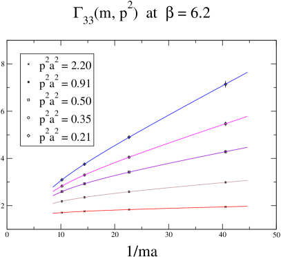
The matrix ${\cal Z}$ of RCs is then extracted from the coefficient $A(p^{2})$ at large $p^{2}$.

As an additional check of this analysis, we study the dependence of the coefficient $B(p^{2})$ on the external momentum. In the right panel of fig. 8 we plot $B_{33}(p^{2})$ at $\beta=6.2$ as a function of $1/(ap)^{2}$ for $(ap)^{2}\geq 0.6$. The solid line in the figure represents the result of the fit to the form

$$B_{33}(p^{2})=\alpha+\frac{\beta}{(ap)^{2}}+\frac{\gamma}{(ap)^{4}}\,.$$ (30)

We find that, within the errors, eq. (30) gives a good description of the data with $\alpha=-0.0009(44)$, a result which is well compatible with zero. This is consistent with the expectation that the Goldstone pole can only appear in power suppressed non-perturbative contributions.

The second approach used to subtract the Goldstone pole is the one suggested in ref. [30] and also discussed in sec. 3.4 for the bilinear pseudoscalar operator. Applied to the case of the four-fermion operators, this method consists in eliminating the contribution of the Goldstone boson by constructing the combinations

$$\Gamma_{ij}^{\rm SUB}(m_{1},m_{2},p^{2})=\frac{m_{1}\,\Gamma_{ij}(m_{1},p^{2})-m_{2}\,\Gamma_{ij}(m_{2},p^{2})}{m_{1}-m_{2}}\,.$$ (31)

The subtracted correlation functions are then extrapolated to the chiral limit by performing a fit to the form

$$\Gamma_{ij}^{\rm SUB}(m_{1},m_{2},p^{2})=\tilde{A}_{ij}(p^{2})+\tilde{C}_{ij}(p^{2})(m_{1}+m_{2})\,.$$ (32)

We find that the results for $\tilde{A}(p^{2})$, obtained from a fit which uses only the four lightest values of quark masses, differ from those of $A(p^{2})$ of eq. (29) by less than 1% in all the range of $p^{2}$ considered in this study. Therefore, at this level of accuracy, the two approaches provide the same estimate of the RCs.

In the PC case also a double Goldstone boson pole can be present. For this reason, we fit in this case the subtracted correlation function of eq. (31) to the form

$$\Gamma_{ij}^{\rm SUB}(m_{1},m_{2},p^{2})=\tilde{A}_{ij}(p^{2})+\tilde{C}_{ij}(p^{2})(m_{1}+m_{2})+\frac{\tilde{E}_{ij}(p^{2})}{m_{1}m_{2}}\,,$$ (33)

which differs from eq. (32) for the presence of the last term. As before, we compute the RCs from the coefficient $\tilde{A}(p^{2})$. Had we used this form in the PV case, a value of $\tilde{E}(p^{2})$ fully compatible with zero would have been obtained. In the PC case instead, our numerical results clearly show the presence of such contribution, which is however much smaller than the single pole contribution proportional to $B(p^{2})$.

Figure 9: $\Delta_{34}$ as function of $\mu$ at $\beta=6.2$ in three cases: without the subtraction of the Goldstone pole (circles), with the subtraction of the single pole (squares) and with the subtraction of both the single and the double poles (diamonds).

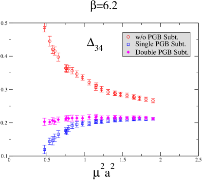
The effect of single and double poles, when not subtracted, is clearly visible in several matrix elements, both of the scale dependent RCs, ${\cal Z}(\mu a,g_{0}^{2})$ and $Z(\mu a,g_{0}^{2})$, and of the scale independent mixing coefficients $\Delta(g_{0}^{2})$. An example of the latter case, namely the one of the matrix element $\Delta_{34}$, is shown in fig. 9. It is very reassuring that $\Delta_{34}$ becomes almost independent of the scale, as should be the case, once the pole contribution has been eliminated. For some other matrix elements, and in particular in the case of $Z_{11}$ and of the corresponding mixing coefficients $\Delta_{1k}$ which are relevant for the lattice estimates of $K^{0}-\bar{K}^{0}$ and $B^{0}-\bar{B}^{0}$ mixing in the Standard Model, the effect of the subtraction of the Goldstone pole is absolutely negligible.

5.3 Renormalization scale dependence, discretization and finite volume effects

In order to investigate the presence of discretization effects and to study the renormalization scale dependence of the RCs of four-fermion operators we follow a procedure close to the one described in sects. 3.1 and 3.3 for the case of bilinear quark operators.

We start by constructing the RGI combinations

$$Z^{RGI}=C^{-1}(\mu){Z}(\mu)$$ (34)

for both the PC and PV operators, where the evolution matrix $C(\mu)$, for the complete basis has been computed, in the ${\rm RI/MOM}$ scheme, at the NLO in perturbation theory [45].

We then rescale the RGI combinations, computed at the different values of the lattice spacing, to a common reference scale $\bar{a}$, which in this case we choose to be the value of the lattice spacing at $\beta=6.45$. To that purpose, we compute the renormalization scale independent ratios

$$R(a,\bar{a})=Z^{RGI}(a)^{-1}Z^{RGI}(\bar{a})=Z(a,\mu)^{-1}Z(\bar{a},\mu)\,.$$ (35)

which are the analogous of those defined in eq. (9) for bilinear operators. We then use these ratios to rescale the RGI RCs at the three values of the coupling different from $\beta=6.45$.

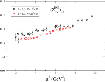
The rescaled RGI combinations should be independent of both the renormalization scale and the lattice spacing. This is true, however, only up to discretization effects and higher-order perturbative corrections not taken into account in the NLO perturbative evaluation of the function $C(\mu)$. A comparison of the rescaled RGI combinations obtained at the same value of the renormalization scale, but at different values of the lattice spacing, provides an estimates of discretization effects. On the other hand, by studying at fixed lattice spacing the dependence of the RGI combinations on the renormalization scale we can investigate the effect of higher orders perturbative contributions not included in the evaluation of the evolution matrix $C(\mu)$.

Figure 10: Results for some of the RGI combinations as obtained at the four values of the lattice coupling and rescaled to $\beta=6.45$.

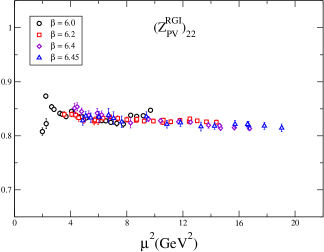
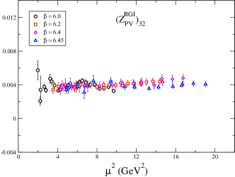
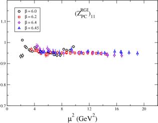
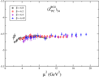
In fig. 10 we show the numerical results for the rescaled RGI combinations, in both the PV and PC cases, as a function of the renormalization scale. In these plots we only show the results for the plus sector. For the minus sector the situation is similar. As can be seen from the plots, most of the matrix elements of both $Z^{RGI}$ and ${\cal Z}^{RGI}$ do not show any significant dependence on the renormalization scale. There are three cases, however, namely the matrix elements 33, 44 and 55, in which the plateau is worse than in the others. Since deviations from the expected constant behaviour are observed in a similar way at all values of the lattice spacing, and the results obtained at different $\beta$ are in good agreement among each others, we conclude that lattice artifacts are quite small and interpret these deviations as mainly due to the effect of N²LO perturbative corrections not included in the evaluation of the function $C(\mu)$. This explanation is also supported by the fact that the operators $Q_{3}$, $Q_{4}$, $Q_{5}$ and ${\cal Q}_{3}$, ${\cal Q}_{4}$, ${\cal Q}_{5}$ have very large anomalous dimensions at the leading order. We emphasize that a better control of the renormalization scale dependence of these operators could be achieved either by a perturbative calculation of the N²LO anomalous dimensions or, even better, by a non-perturbative study of the running by using an iterative matching technique which involves several lattice scales. This approach, which has been already implemented within the context of the SF scheme (see for instance ref. [19] for a study of the pseudoscalar RC $Z_{P}$) can be implemented with other NPR techniques as well, like the ${\rm RI/MOM}$ or the $x$-space method.

In fig. 11 we show the results for the mixing coefficients $\Delta$ as a function of the renormalization scale $\mu$. At fixed lattice spacing, these quantities are expected to be independent of $\mu$. Indeed, in most of the cases we observe from the plots a reasonably good scale independence at large $p^{2}$, in particular for those coefficients of relatively large magnitude. The systematic error induced by the effect of a residual scale dependence is accounted for in the final determination of the RCs.

Figure 11: Results for some of the mixing coefficients $\Delta_{ij}$ at the four values of lattice coupling.

Figure 12: Results for some of the matrix elements of $\Delta$ (left) and for the ratios $\Delta/g^{2}_{plaq}$ (right), where $g^{2}_{plaq}=g^{2}/(\frac{1}{3}{\rm Tr}(U_{P}))$ is the boosted coupling defined from the plaquette, as a function of the lattice spacing.

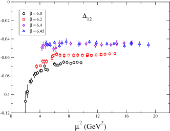
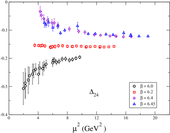
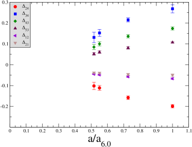
Mixing among operators of different naive chirality, parameterized by the matrix $\Delta$, is a consequence of the explicit chiral symmetry breaking induced by the Wilson term. Therefore this mixing is expected to disappear in the continuum limit. To verify this expectation, we show in the left plot of fig. 12 the results for some of the matrix elements of $\Delta$ as a function of the lattice spacing. We see from this plot that the absolute values of the $\Delta$s decrease as the continuum limit is approached. In the right panel of fig. 12 we present the same matrix elements of $\Delta$ divided by $g^{2}_{plaq}$, where $g^{2}_{plaq}=g^{2}/(\frac{1}{3}{\rm Tr}(U_{P}))$ is the boosted coupling defined from the plaquette. If the perturbative expansion in terms of $g^{2}_{plaq}$ is rapidly convergent, the ratios $\Delta/g^{2}_{plaq}$ are expected to be flatter than the $\Delta$s themselves. The plot in fig. 12 shows that this is indeed the case. The residual dependence on the lattice spacing, observed in the figure, signals the presence either of higher orders in the perturbative expansion or of finite lattice spacing effects.

To conclude the analysis of the systematic errors which may affect the determination of the RCs of four-fermion operators we investigate the presence of finite volume effects. As already done for bilinear quark operators (see sec. 3.6), we compare the results for the RCs obtained at $\beta=6.0$ on two different volumes, namely $16^{3}\times 52$ and $24^{3}\times 64$. The parameters of the simulation on the smallest volume are those given in table 1. For the calculation on the largest volume, we have used a set of 480 gauge field configurations and computed quark propagators at four values of the Wilson parameter, namely $\kappa=$0.13180, 0.13280, 0.13770, 0.13440 ($\kappa_{cr}=0.135220(6)$). The comparison of the results is illustrated in fig. 13 for some of the matrix elements of the RCs and mixing coefficients.

Figure 13: Comparison for some of the matrix elements of the RCs and mixing coefficients as obtained on two different volumes at $\beta=6.0$.

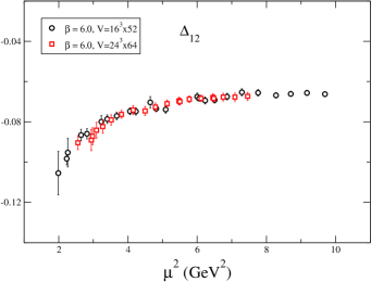
We see from the plots that, in some cases, the presence of finite volume effects is visible, though they become negligible at large values of the renormalization scale ($\mu\mathrel{\hbox to0.0pt{\raise 2.20013pt\hbox{$>$}\hss}{\lower 2.20013pt\hbox{$\sim$}}}2.5\,{\rm GeV}$). Since our final determination of the RCs is obtained from a fit in the interval $\mu=[2.5,3.0]\,{\rm GeV}$ (see below), we find that the results obtained on the different volumes are compatible within the statistical and the estimated systematic errors. For this reason, we do not include in the final error any additional uncertainty due to final volume effects, although this point would require more investigations. In order to better illustrate this comparison, when quoting our final results (see tables 4-7) we will present at $\beta=6.0$ the determinations obtained on both the lattices with different size.

5.4 Results

In order to obtain the RCs at a given scale we proceed in the following way. We extract the RGI combinations $Z^{RGI}$ and ${\cal Z}^{RGI}$ by fitting to a constant the plateau in fig. 10, and similarly for the other matrix elements, in the interval $\mu=[2.5,3.0]\,{\rm GeV}$. We then use the renormalization group evolution at the NLO to obtain the value of the RCs at the desired scale. A standard choice of the scale, at which matrix elements are matched with Wilson coefficients in the effective weak Hamiltonian, is $\mu=2\,{\rm GeV}$. Since this value lies in most of the cases within the range of momenta at which the RCs are directly computed, we estimate the systematic error in the following way: we take the RCs computed non-perturbatively at a given scale $\mu_{0}$ and run them up or down to the desired scale $\mu=2\,{\rm GeV}$. The systematic error is then estimated from the deviations of the results obtained by performing different choices of $\mu_{0}$. The same procedure has been also applied for the determinations of the mixing coefficients $\Delta$s. The only difference is that, being free of anomalous dimension, these quantities do not evolve with the renormalization scale.

We emphasize that the systematic error induced by the renormalization group running of the RCs should be regarded as an uncertainty related mainly to the perturbative estimates of the Wilson coefficients of the effective Hamiltonian, rather than to the non-perturbative the determination of the RCs. Indeed, had we chosen to quote the values of the RCs at the renormalization scale at which they are directly determined in the lattice calculation, this error would be absent.

Our final estimates of the RCs of four-fermion operators in the ${\rm RI/MOM}$ scheme at the scale $\mu=2\,{\rm GeV}$ are collected in tables 4, 5, 6 and 7 for the PC^± and PV^± respectively. As mentioned before, for the case of $\beta=6.0$, we present the results obtained on lattices with two different sizes.

$\beta$	$6.0\,(16^{3}\times 52)$	$6.0\,(24^{3}\times 64)$	$6.2$	$6.4$	$6.45$
$Z_{11}$	$0.609(4)(13)$	$0.604(3)(4)$	$0.634(5)(5)$	$0.671(10)(9)$	$0.682(7)(5)$
$\Delta_{12}$	-0.067( 1)( 4)	-0.068( 2)( 4)	-0.058( 2)( 4)	-0.048( 1)( 3)	-0.045( 2)( 2)
$\Delta_{13}$	-0.021( 1)( 1)	-0.022( 1)( 1)	-0.016( 1)( 2)	-0.012( 1)( 2)	-0.012( 1)( 2)
$\Delta_{14}$	0.010( 1)( 3)	0.014( 1)( 3)	0.011( 2)( 4)	0.013( 1)( 3)	0.013( 1)( 3)
$\Delta_{15}$	0.004( 1)( 3)	0.003( 1)( 2)	0.006( 1)( 1)	0.004( 2)( 1)	0.006( 1)( 3)
$Z_{22}$	$0.669(3)(11)$	$0.662(3)(3)$	$0.691(3)(5)$	$0.732(8)(10)$	$0.740(8)(7)$
$Z_{23}$	$0.274(2)(8)$	$0.276(2)(2)$	$0.298(4)(7)$	$0.323(8)(9)$	$0.328(6)(10)$
$\Delta_{21}$	-0.050( 1)( 6)	-0.053( 1)( 5)	-0.047( 2)( 5)	-0.040( 1)( 4)	-0.038( 1)( 3)
$\Delta_{24}$	-0.199( 4)( 7)	-0.194( 3)( 3)	-0.158( 6)( 7)	-0.111( 2)(12)	-0.102( 4)(17)
$\Delta_{25}$	0.020( 1)( 2)	0.019( 1)( 1)	0.013( 1)( 3)	0.008( 1)( 3)	0.008( 1)( 4)
$Z_{32}$	$0.029(1)(1)$	$0.028(1)(1)$	$0.025(1)(1)$	$0.024(2)(1)$	$0.022(1)(1)$
$Z_{33}$	$0.390(3)(31)$	$0.376(2)(15)$	$0.357(4)(19)$	$0.344(5)(12)$	$0.331(6)(18)$
$\Delta_{31}$	0.014( 1)( 4)	0.015( 1)( 3)	0.015( 1)( 3)	0.013( 1)( 1)	0.013( 0)( 3)
$\Delta_{34}$	0.269( 6)(18)	0.260( 4)( 3)	0.215( 7)( 7)	0.153( 3)(16)	0.131( 7)(24)
$\Delta_{35}$	-0.009( 0)( 1)	-0.008( 1)( 1)	-0.006( 1)( 1)	-0.003( 1)( 2)	-0.002( 1)( 5)
$Z_{44}$	$0.478(3)(33)$	$0.463(2)(15)$	$0.445(4)(20)$	$0.434(5)(14)$	$0.419(5)(21)$
$Z_{45}$	$-0.024(1)(1)$	$-0.023(1)(1)$	$-0.019(1)(1)$	$-0.017(2)(2)$	$-0.015(2)(1)$
$\Delta_{41}$	0.005( 0)( 2)	0.005( 0)( 2)	0.006( 0)( 2)	0.005( 0)( 1)	0.005( 0)( 1)
$\Delta_{42}$	0.007( 0)( 2)	0.006( 0)( 0)	0.006( 1)( 0)	0.005( 1)( 2)	0.003( 1)( 3)
$\Delta_{43}$	0.174( 4)( 6)	0.164( 2)( 3)	0.136( 4)( 7)	0.100( 2)(10)	0.085( 5)(11)
$Z_{54}$	$-0.253(2)(13)$	$-0.257(2)(6)$	$-0.291(3)(10)$	$-0.329(6)(13)$	$-0.337(6)(13)$
$Z_{55}$	$0.786(4)(15)$	$0.788(3)(9)$	$0.852(5)(19)$	$0.934(12)(23)$	$0.953(9)(19)$
$\Delta_{51}$	0.005( 0)( 3)	0.005( 1)( 2)	0.007( 1)( 2)	0.007( 1)( 1)	0.007( 0)( 2)
$\Delta_{52}$	0.013( 0)( 1)	0.012( 0)( 1)	0.009( 1)( 1)	0.006( 1)( 2)	0.006( 1)( 2)
$\Delta_{53}$	0.107( 2)( 2)	0.100( 2)( 3)	0.081( 2)( 6)	0.060( 1)( 6)	0.052( 3)( 6)

Table 4: Results for the RCs of the PC${}^{\,+}$ sector in the ${\rm RI/MOM}$ scheme at the scale $\mu$=2 GeV.

$\beta$	$6.0\,(16^{3}\times 52)$	$6.0\,(24^{3}\times 64)$	$6.2$	$6.4$	$6.45$
$Z_{11}$	$0.622(3)(10)$	$0.614(3)(3)$	$0.621(5)(7)$	$0.641(8)(8)$	$0.642(13)(9)$
$\Delta_{12}$	-0.033( 1)( 6)	-0.034( 1)( 5)	-0.029( 1)( 4)	-0.026( 1)( 4)	-0.025( 1)( 3)
$\Delta_{13}$	0.010( 1)( 3)	0.007( 1)( 1)	0.005( 1)( 3)	0.008( 1)( 1)	0.001( 2)( 6)
$\Delta_{14}$	-0.007( 1)( 9)	-0.013( 1)( 6)	-0.016( 2)( 6)	-0.019( 1)( 5)	-0.018( 2)( 5)
$\Delta_{15}$	-0.003( 1)( 9)	-0.007( 1)( 6)	-0.012( 2)( 5)	-0.017( 2)( 6)	-0.017( 3)( 6)
$Z_{22}$	$0.677(3)(9)$	$0.669(2)(3)$	$0.700(4)(5)$	$0.743(9)(11)$	$0.749(8)(7)$
$Z_{23}$	$-0.277(2)(10)$	$-0.282(2)(5)$	$-0.306(4)(9)$	$-0.335(8)(12)$	$-0.340(5)(10)$
$\Delta_{21}$	-0.045( 1)( 3)	-0.050( 2)( 3)	-0.040( 2)( 3)	-0.033( 1)( 1)	-0.028( 2)( 4)
$\Delta_{24}$	0.138( 2)( 6)	0.134( 3)( 1)	0.113( 3)( 5)	0.078( 2)( 8)	0.064( 5)(13)
$\Delta_{25}$	0.012( 1)( 3)	0.012( 1)( 1)	0.010( 1)( 2)	0.007( 1)( 4)	0.005( 1)( 5)
$Z_{32}$	$-0.027(1)(1)$	$-0.028(1)(1)$	$-0.023(1)(1)$	$-0.021(2)(1)$	$-0.021(1)(2)$
$Z_{33}$	$0.402(3)(30)$	$0.386(2)(14)$	$0.366(4)(19)$	$0.349(5)(13)$	$0.335(7)(19)$
$\Delta_{31}$	-0.008( 1)( 5)	-0.011( 1)( 1)	-0.007( 1)( 2)	-0.003( 1)( 3)	-0.004( 2)( 5)
$\Delta_{34}$	0.203( 3)( 9)	0.195( 3)( 3)	0.163( 4)( 9)	0.115( 3)(13)	0.094( 8)(18)
$\Delta_{35}$	0.000( 0)( 6)	0.000( 1)( 2)	-0.002( 1)( 2)	-0.002( 1)( 4)	-0.005( 2)( 9)
$Z_{44}$	$0.309(5)(44)$	$0.300(3)(15)$	$0.280(5)(20)$	$0.258(5)(16)$	$0.238(7)(37)$
$Z_{45}$	$-0.007(1)(3)$	$-0.007(1)(1)$	$-0.016(1)(2)$	$-0.020(2)(1)$	$-0.019(4)(18)$
$\Delta_{41}$	0.004( 2)(32)	0.000( 1)( 1)	0.002( 1)( 4)	0.003( 2)( 4)	-0.021(14)(63)
$\Delta_{42}$	-0.010( 1)( 7)	-0.012( 1)( 2)	-0.004( 1)( 4)	0.000( 2)(13)	-0.001(10)(55)
$\Delta_{43}$	0.331(18)(85)	0.303( 5)( 6)	0.248( 9)( 5)	0.174( 4)(19)	0.165(22)(184)
$Z_{54}$	$0.120(2)(3)$	$0.124(2)(1)$	$0.133(3)(3)$	$0.139(5)(2)$	$0.133(7)(15)$
$Z_{55}$	$0.713(3)(10)$	$0.712(3)(5)$	$0.745(4)(16)$	$0.800(12)(18)$	$0.804(13)(26)$
$\Delta_{51}$	-0.003( 1)( 6)	-0.005( 1)( 4)	-0.010( 1)( 3)	-0.014( 1)( 4)	-0.014( 2)( 4)
$\Delta_{52}$	0.013( 1)( 1)	0.013( 1)( 1)	0.009( 1)( 2)	0.007( 1)( 2)	0.006( 1)( 4)
$\Delta_{53}$	-0.113( 3)( 5)	-0.107( 2)( 2)	-0.087( 3)( 5)	-0.064( 1)( 6)	-0.058( 2)( 6)

Table 5: Results for the RCs of the PC${}^{\,-}$ sector in the ${\rm RI/MOM}$ scheme at the scale $\mu$=2 GeV.

$\beta$	$6.0\,(16^{3}\times 52)$	$6.0\,(24^{3}\times 64)$	$6.2$	$6.4$	$6.45$
$Z_{11}$	$0.608(4)(14)$	$0.604(3)(5)$	$0.635(5)(4)$	$0.671(9)(8)$	$0.681(7)(3)$
$Z_{22}$	$0.673(3)(10)$	$0.666(3)(3)$	$0.697(4)(3)$	$0.738(8)(11)$	$0.744(8)(9)$
$Z_{23}$	$0.279(2)(9)$	$0.281(2)(3)$	$0.307(4)(9)$	$0.334(8)(11)$	$0.335(6)(10)$
$Z_{32}$	$0.028(1)(1)$	$0.028(1)(1)$	$0.024(1)(1)$	$0.023(2)(1)$	$0.021(1)(2)$
$Z_{33}$	$0.392(3)(28)$	$0.375(3)(14)$	$0.353(4)(21)$	$0.338(4)(14)$	$0.331(6)(17)$
$Z_{44}$	$0.476(3)(30)$	$0.457(3)(15)$	$0.437(4)(22)$	$0.425(5)(16)$	$0.417(5)(22)$
$Z_{45}$	$-0.024(1)(1)$	$-0.022(1)(1)$	$-0.019(1)(1)$	$-0.016(2)(1)$	$-0.015(2)(3)$
$Z_{54}$	$-0.255(2)(11)$	$-0.260(2)(5)$	$-0.295(3)(12)$	$-0.333(6)(14)$	$-0.339(6)(13)$
$Z_{55}$	$0.787(4)(15)$	$0.790(3)(9)$	$0.854(5)(19)$	$0.936(12)(24)$	$0.952(10)(19)$

Table 6: Results for the RCs of the PV${}^{\,+}$ sector in the ${\rm RI/MOM}$ scheme at the scale $\mu$=2 GeV.

$\beta$	$6.0\,(16^{3}\times 52)$	$6.0\,(24^{3}\times 64)$	$6.2$	$6.4$	$6.45$
$Z_{11}$	$0.623(3)(10)$	$0.614(3)(4)$	$0.621(5)(5)$	$0.642(8)(8)$	$0.642(11)(8)$
$Z_{22}$	$0.673(3)(10)$	$0.666(3)(4)$	$0.696(4)(3)$	$0.737(8)(11)$	$0.744(8)(9)$
$Z_{23}$	$-0.279(2)(9)$	$-0.281(2)(3)$	$-0.307(4)(9)$	$-0.333(8)(12)$	$-0.335(6)(10)$
$Z_{32}$	$-0.028(1)(1)$	$-0.028(1)(1)$	$-0.024(1)(1)$	$-0.023(2)(1)$	$-0.021(1)(2)$
$Z_{33}$	$0.392(3)(28)$	$0.375(3)(14)$	$0.353(4)(21)$	$0.338(4)(14)$	$0.331(6)(17)$
$Z_{44}$	$0.312(3)(36)$	$0.295(3)(16)$	$0.271(4)(22)$	$0.249(4)(21)$	$0.218(15)(80)$
$Z_{45}$	$-0.006(1)(3)$	$-0.007(1)(1)$	$-0.016(1)(3)$	$-0.020(2)(1)$	$-0.020(5)(52)$
$Z_{54}$	$0.126(1)(4)$	$0.126(2)(1)$	$0.135(3)(3)$	$0.140(5)(1)$	$0.130(10)(36)$
$Z_{55}$	$0.715(3)(12)$	$0.714(3)(7)$	$0.746(4)(17)$	$0.802(12)(18)$	$0.806(16)(32)$

Table 7: Results for the RCs of the PV${}^{\,-}$ sector in the ${\rm RI/MOM}$ scheme at the scale $\mu$=2 GeV.

Conclusions

In this paper we have presented the results of an extensive lattice calculation of the RCs of bilinear and four-quark $\Delta F=2$ and $\Delta I=3/2$ operators by using the ${\rm RI/MOM}$ NPR method. Several sources of systematic errors, including discretization errors and finite volume effects, have been investigated. When possible, we have also compared the results with those obtained by using other non-perturbative approaches, like the WI and the SF methods. In these cases, we find an agreement which is typically at the level of 1%. This comparison supports the conclusion that the ${\rm RI/MOM}$ method allows to obtain an accurate non-perturbative determination of the RCs of lattice operators. At the same time, the method is extremely simple to implement and can be applied to a large class of operators. The only notable exception is represented by those operators the renormalization of which requires subtraction of power divergences. In the latter case, and in particular in the case of the $\Delta I=1/2$ four-fermion operators, the use of non gauge invariant correlation functions renders the applicability of the ${\rm RI/MOM}$ method extremely difficult, if not impossible in practice. In order to renormalize these operators the gauge invariant NPR method in $x$-space [4]-[6] might be the method of choice.

Appendix A

In this appendix we show that the RCs of bilinear quark operators obtained with the ${\rm RI/MOM}$ method in the chiral limit, at sufficiently large values of the external momentum and at zero momentum transfer, are automatically improved at ${\cal O}(a)$.

The renormalized and improved version of the bilinear operator $O_{\Gamma}={\overline{q}}\Gamma q$ has the form [46]:

$$\widehat{O}_{\Gamma}^{I}=Z_{\Gamma}O_{\Gamma}^{I}=Z_{\Gamma}\left(\,{\overline{q}}\Gamma q\,+\,a\,c_{\Gamma}O_{4,\Gamma}\,+\,a\,{c^{\prime}\!}_{\Gamma}E_{\Gamma}\right)$$ (36)

where $Z_{\Gamma}$ is the multiplicative RC in which we also include here the ${\cal O}(a)$ linear dependence on the quark mass, $Z_{\Gamma}=Z^{0}_{\Gamma}\left(1+b_{\Gamma}am\right)$. The coefficients $b_{\Gamma}$, $c_{\Gamma}$, ${c^{\prime}\!}_{\Gamma}$ express the mixing of $O_{\Gamma}$ with higher-dimension operators. This mixing has to be taken into account in order to improve the operator at ${\cal O}(a)$. The operator $E_{\Gamma}$ in eq. (36) is given by:

$$E_{\Gamma}={\overline{q}}\left[\Gamma({\overrightarrow{\hbox to0.0pt{\hbox to8.55695pt{\hfil/\hfil}\hss}D}}+m_{0})+(-{\overleftarrow{\hbox to0.0pt{\hbox to8.55695pt{\hfil/\hfil}\hss}D}}+m_{0})\Gamma\right]q$$ (37)

where ${\overrightarrow{\hbox to0.0pt{\hbox to8.55695pt{\hfil/\hfil}\hss}D}}+m_{0}$ is a shorthand for the entire lattice fermion operator, including the Wilson and the SW-clover terms. Therefore $E_{\Gamma}$ vanishes by the equation of motion and it only contributes to contact terms when inserted in correlation functions. The operator $O_{4,\Gamma}$ in eq. (36) is a gauge-invariant, dimension-four operator which does not vanish by the equation of motion. In the cases of the vector, axial-vector and tensor operators, $O_{4,\Gamma}$ is given by

$$O_{4,V} = \partial_{\nu}\,({\overline{q}}\sigma_{\mu,\nu}q)$$

$$O_{4,A} = \partial_{\mu}\,({\overline{q}}\gamma^{5}q)$$ (38)

$$O_{4,T} = \partial_{\mu}\,({\overline{q}}\gamma_{\nu}q)-\partial_{\nu}\,({\overline{q}}\gamma_{\mu}q)$$

while this mixing is absent for the scalar and pseudoscalar densities.

In order to improve the off-shell correlation functions, we also consider the renormalized improved quark and antiquark fields [46],

$$\widehat{q} = Z_{q}^{-1/2}\left[1+a\,{c^{\prime}\!}_{q}({\overrightarrow{\hbox to0.0pt{\hbox to8.55695pt{\hfil/\hfil}\hss}D}}+m_{0})+a\,c_{\scriptstyle{\rm NGI}}{\overrightarrow{\hbox to0.0pt{\hbox to5.30904pt{\hfil/\hfil}\hss}\partial}}\right]q$$ (39)

$$\widehat{\overline{q}} = Z_{q}^{-1/2}\,{\overline{q}}\left[1+a\,{c^{\prime}\!}_{q}(-{\overleftarrow{\hbox to0.0pt{\hbox to8.55695pt{\hfil/\hfil}\hss}D}}+m_{0})-a\,c_{\scriptstyle{\rm NGI}}{\overleftarrow{\hbox to0.0pt{\hbox to5.30904pt{\hfil/\hfil}\hss}\partial}}\right]$$

with $Z_{q}=Z^{0}_{q}\left(1+b_{q}am\right)$. In terms of these fields we can define the renormalized improved quark propagator:

$$\widehat{S}(p)=\int d^{4}x\,e^{-ip\cdot x}\,\langle\widehat{q}(x)\widehat{\overline{q}}(0)\rangle\,,$$ (40)

which, by using eq. (39), can be related to the corresponding lattice quantity $S(p)$ by

$$\widehat{S}(p)=Z_{q}^{-1}\,\left[S(p)+2a\,{c^{\prime}\!}_{q}+2a\,c_{\scriptstyle{\rm NGI}}\,i\hbox to0.0pt{\hbox to5.03125pt{\hfil/\hfil}\hss}p\,S(p)\right]\,$$ (41)

up to ${\cal O}(a^{2})$ terms.

Let us now discuss the effect of the off-shell improvement, defined by eqs. (36) and (39), in the determination of the RCs with the ${\rm RI/MOM}$ method. The relevant renormalized improved correlation function is defined in terms of improved operators and external fields:

$${G}_{\Gamma}^{I}(p,p^{\prime})=\int d^{4}x\,d^{4}y\,e^{-ip\cdot x+ip^{\prime}\cdot y}\,\langle\widehat{q}(x)O_{\Gamma}^{I}(0)\widehat{\overline{q}}(y)\rangle=$$

$$\qquad\int d^{4}x\,d^{4}y\,e^{-ip\cdot x+ip^{\prime}\cdot y}\,\langle\widehat{q}(x)\left({\overline{q}}\Gamma q\,+\,a\,c_{\Gamma}O_{4,\Gamma}\,+\,a\,{c^{\prime}\!}_{\Gamma}E_{\Gamma}\right)_{0}\widehat{\overline{q}}(y)\rangle\,.$$ (42)

The ${\rm RI/MOM}$ method consists in imposing that the forward amputated Green function,

$$\Lambda_{\Gamma}^{I}(p)=\widehat{S}(p)^{-1}{G}_{\Gamma}^{I}(p,p)\widehat{S}(p)^{-1}\,,$$ (43)

computed in a fixed gauge and renormalized at a given scale $p^{2}=\mu^{2}$, is equal to its tree-level value. In practice, this condition is implemented by requiring:

$$Z_{\Gamma}\,\Gamma_{\Gamma}^{I}(p)|_{p^{2}=\mu^{2}}=Z_{\Gamma}\,\hbox{\rm Tr}\,[\Lambda_{\Gamma}^{I}(p)\,P_{\Gamma}]|_{p^{2}=\mu^{2}}=1$$ (44)

where $P_{\Gamma}$ is the Dirac projector.

The Green functions $G_{\Gamma}^{I}(p)$ and $\Lambda_{\Gamma}^{I}(p)$ can be easily related to their unimproved counterparts. By using eqs. (36)-(42), and up to terms of ${\cal O}(a^{2})$, one finds:

$$G_{\Gamma}^{I}(p) = G_{\Gamma}(p)\,+\,a\,c_{\Gamma}\,G_{4,\Gamma}(p)\,+\,a\,({c^{\prime}\!}_{\Gamma}+{c^{\prime}\!}_{q})\left(\Gamma\,\widehat{S}(p)+\widehat{S}(p)\Gamma\right)+$$ (45)

$$a\,c_{\scriptstyle{\rm NGI}}\left(i\hbox to0.0pt{\hbox to5.03125pt{\hfil/\hfil}\hss}p\,G_{\Gamma}^{I}(p)+G_{\Gamma}^{I}(p)\,i\hbox to0.0pt{\hbox to5.03125pt{\hfil/\hfil}\hss}p\right)$$

where $G_{\Gamma}(p)$ is the Green function of the unimproved operator $O_{\Gamma}$, constructed with unimproved external quark fields, and $G_{4,\Gamma}(p)$ is the analogous quantity for the operator $O_{4,\Gamma}$ defined in eq. (36). The improved function $\Lambda_{\Gamma}^{I}(p)$ is then obtained from $G_{\Gamma}^{I}(p)$ by amputating the external legs with improved quark propagators, according to eq. (43). The result is:

$$\Lambda_{\Gamma}^{I}(p)=\Lambda_{\Gamma}(p)\,+\,a\,c_{\Gamma}\,\Lambda_{4,\Gamma}(p)\,+\,a\,({c^{\prime}\!}_{\Gamma}+{c^{\prime}\!}_{q})\left(\Gamma\,\widehat{S}(p)^{-1}+\widehat{S}(p)^{-1}\Gamma\right)-$$

$$\qquad 2a\,{c^{\prime}\!}_{q}\,Z_{q}^{-1}\left(\widehat{S}(p)^{-1}\Lambda_{\Gamma}^{I}(p)+\Lambda_{\Gamma}^{I}(p)\widehat{S}(p)^{-1}\right)-a\,c_{\scriptstyle{\rm NGI}}\left(i\hbox to0.0pt{\hbox to5.03125pt{\hfil/\hfil}\hss}p\,\Lambda_{\Gamma}^{I}(p)+\Lambda_{\Gamma}^{I}(p)\,i\hbox to0.0pt{\hbox to5.03125pt{\hfil/\hfil}\hss}p\right)$$ (46)

Finally, by projecting eq. (46) onto the tree-level form factor with the projector $P_{\Gamma}$, one obtains:

$$\Gamma_{\Gamma}^{I}(p)=\Gamma_{\Gamma}(p)\,+\,a\,c_{\Gamma}\,\Gamma_{4,\Gamma}(p)\,+\,2\,a\,({c^{\prime}\!}_{\Gamma}+{c^{\prime}\!}_{q})\hbox{\rm Tr}\,[\widehat{S}(p)^{-1}]-$$

$$\qquad 2a\,{c^{\prime}\!}_{q}\,Z_{q}^{-1}\hbox{\rm Tr}\,\left(\widehat{S}(p)^{-1}\,\Lambda_{\Gamma}^{I}(p)\,P_{\Gamma}-\Lambda_{\Gamma}^{I}(p)\,\widehat{S}(p)^{-1}\,P_{\Gamma}\right)+$$

$$\qquad a\,c_{\scriptstyle{\rm NGI}}\hbox{\rm Tr}\,\left(i\hbox to0.0pt{\hbox to5.03125pt{\hfil/\hfil}\hss}p\,\Lambda_{\Gamma}^{I}(p)\,P_{\Gamma}+\Lambda_{\Gamma}^{I}(p)\,i\hbox to0.0pt{\hbox to5.03125pt{\hfil/\hfil}\hss}p\,P_{\Gamma}\right)\,.$$ (47)

The various contributions to the amputated projected Green function in eq. (47) are easily identified. The third term on the r.h.s. of eq. (47) comes from the operators vanishing by the equation of motion and it is proportional to the trace of the improved inverse quark propagator. Since at large values of $p^{2}$ this quantity is proportional to the quark mass, such a term does not affect the determination of the renormalization constants in the chiral limit.

One may be easily convinced that also the last two terms in eq. (47) proportional to ${c^{\prime}\!}_{q}$ and $c_{\scriptstyle{\rm NGI}}$ respectively, vanish in this limit. We first observe that, for vanishing quark mass, the improved propagator $\widehat{S}(p)^{-1}$ at large $p^{2}$ is proportional to $\hbox to0.0pt{\hbox to5.03125pt{\hfil/\hfil}\hss}p$. Therefore, the two terms have the same form. In addition, we note that contributions from $\Lambda_{\Gamma}^{I}(p)$ proportional to the tree-level form factor, $\Gamma$, vanish because they reduce to $\hbox{\rm Tr}\,(\hbox to0.0pt{\hbox to5.03125pt{\hfil/\hfil}\hss}p)$. For the same reason, one also finds the vanishing of all possible contributions coming from different (dimensionless) form factor which do not depend on the quark mass. For instance, in the case of the vector current, the Green function $\Lambda_{\mu}^{I}(p)$ also contains a term proportional to $p_{\mu}\hbox to0.0pt{\hbox to5.03125pt{\hfil/\hfil}\hss}p/p^{2}$, which again gives a contribution vanishing as $\hbox{\rm Tr}\,(\hbox to0.0pt{\hbox to5.03125pt{\hfil/\hfil}\hss}p)$ to the last two terms of eq. (47). A non vanishing contribution may come from a form factor proportional to $m\hbox to0.0pt{\hbox to5.03125pt{\hfil/\hfil}\hss}p\gamma_{\mu}/p^{2}$, but then this contribution vanishes in the chiral limit.

In the case of the vector, axial-vector and tensor operators, on-shell ${\cal O}(a)$-improvement also requires to consider the mixing of the bare operators $O_{\Gamma}$ with the dimension-4 operators $O_{4,\Gamma}$, whose contribution is represented by the second term on the r.h.s. of eq. (47). For the scalar and pseudoscalar densities this mixing is absent. In the other cases, the operators $O_{4,\Gamma}$ are listed in eq. (Appendix A). A simple observation is that the operators $O_{4,\Gamma}$ all have the form of a 4-divergence. Therefore, their forward correlation functions, $\Gamma_{4,\Gamma}(p)$ in eq. (47), vanish identically. This completes the proof that only the unimproved correlator $\Gamma_{\Gamma}(p)$ survives at large $p^{2}$ and in the chiral limit on the r.h.s. of eq. (47) and contributes to the calculation of the RCs with the ${\rm RI/MOM}$ method. Such a calculation can thus be performed even in the lacking of a non-perturbative determination of the coefficients $c_{\Gamma}$ and ${c^{\prime}\!}_{\Gamma}$. Note also that, although the correlation function $\Gamma_{\Gamma}^{I}(p)$ is obtained from $G_{\Gamma}^{I}(p,p)$ by amputating the external legs with improved quark propagators, in practice, in the chiral limit, improving the quark propagator is also an unnecessary step for the determination of the RCs.

Appendix B

In this appendix we show that, in the case of four-fermion operators, both single and double Goldstone boson poles can appear in the chiral limit in the relevant correlation functions, and may thus affect the ${\rm RI/MOM}$ NPR procedure at finite values of the external momenta. For convenience, we work with non vanishing quark masses and we will consider the zero quark mass limit only at the end of the calculation.

Let us consider the Green function of a four fermion operator ${\cal O}_{i}$ with four external quark states and two different external momenta

$$G_{i}(p,p^{\prime}) = \int d^{4}x_{1}\,d^{4}x_{2}\,d^{4}x_{3}\,d^{4}x_{4}\,e^{-ip(x_{1}+x_{3})+ip^{\prime}(x_{2}+x_{4})}\,\times$$ (48)

$$\langle 0|T[\psi^{a}(x_{1})\,\bar{\psi}^{b}(x_{2})\,{\cal O}_{i}(0)\,\psi^{c}(x_{3})\,\bar{\psi}^{d}(x_{4})]|0\rangle$$

$$\equiv \langle 0|T[\tilde{\psi^{a}}(p)\,\tilde{\bar{\psi}^{b}}(p^{\prime})\,{\cal O}_{i}(0)\,\tilde{\psi^{c}}(p)\,\tilde{\bar{\psi}^{d}}(p^{\prime})]|0\rangle$$

By applying the LSZ reduction formula we can write

$$G_{i}(p,p^{\prime}) = \langle 0|T[\psi^{a}(0)\,\tilde{\bar{\psi}^{b}}(p^{\prime})]|\pi^{ba}(q)\rangle\,\frac{i}{q^{2}-m_{\pi}^{2}}\,\langle\pi^{ba}(q)|T[{\cal O}_{i}(0)\,\tilde{\psi^{c}}(p)\,\tilde{\bar{\psi}^{d}}(p^{\prime})]|0\rangle\,+$$ (49)

$$NP\left[\langle 0|T[\tilde{\psi^{a}}(p)\,\tilde{\bar{\psi}^{b}}(p^{\prime})\,{\cal O}_{i}(0)\,\tilde{\psi^{c}}(p)\,\tilde{\bar{\psi}^{d}}(p^{\prime})]|0\rangle\right]\,+\,\ldots$$

where $q_{\mu}=p_{\mu}-p^{\prime}_{\mu}$ and we have identified the Goldstone boson with the $\pi$ meson. In eq. (49) the symbol $NP[\dots]$ indicates the part of the correlation function without pions in the intermediate states and the dots represent terms with pion propagators corresponding to pions different from $|\pi^{ba}(q)\rangle$ (i.e. $|\pi^{da}(q)\rangle$, $|\pi^{cd}(q)\rangle$ and $|\pi^{bc}(q)\rangle$). If we now apply the reduction formula again we obtain

$$G_{i}(p,p^{\prime})=\langle 0|T[\psi^{a}(0)\tilde{\bar{\psi}^{b}}(p^{\prime})]|\pi^{ba}(q)\rangle\frac{i}{q^{2}-m_{\pi}^{2}}\,\times$$

$$\qquad\left\{\langle\pi^{ba}(q)|{\cal O}_{i}(0)|\pi^{cd}(q)\rangle\frac{i}{q^{2}-m_{\pi}^{2}}\langle\pi^{cd}(q)|T[\psi^{c}(0)\tilde{\bar{\psi}^{d}}(p^{\prime})]|0\rangle\,+\right.$$

$$\qquad\left.NP\left[\langle\pi^{ba}(q)|T[{\cal O}_{i}(0)\tilde{\psi}^{c}(p)\tilde{\bar{\psi}^{d}}(p^{\prime})]|0\rangle\right]\right\}+\ldots\,.$$ (50)

In the implementation of the ${\rm RI/MOM}$ method we have considered the case $p_{\mu}=p^{\prime}_{\mu}$, corresponding to $q_{\mu}=0$. From eq. (Appendix B) it is then clear that both single and double pion poles can appear in the amputated Green functions in the chiral limit. In the case of parity violating operators, however, since by parity $\langle\pi^{ba}(0)|{\cal O}_{i}^{PV}(0)|\pi^{cd}(0)\rangle=0$, only single poles can be present.

References

- [1] M. Bochicchio, L. Maiani, G. Martinelli, G. C. Rossi and M. Testa, Nucl. Phys. B 262 (1985) 331.
- [2] G. Martinelli, C. Pittori, C. T. Sachrajda, M. Testa and A. Vladikas, Nucl. Phys. B 445 (1995) 81 [hep-lat/9411010].
- [3] K. Jansen et al., Phys. Lett. B 372 (1996) 275 [hep-lat/9512009].
- [4] G. Martinelli, G. C. Rossi, C. T. Sachrajda, S. R. Sharpe, M. Talevi and M. Testa, Phys. Lett. B 411 (1997) 141 [hep-lat/9705018].
- [5] D. Becirevic, V. Gimenez, V. Lubicz, G. Martinelli, M. Papinutto, J. Reyes and C. Tarantino [SPQcdR Collaboration], Nucl. Phys. Proc. Suppl. 119 (2003) 442 [hep-lat/0209168].
- [6] V. Gimenez et al., Nucl. Phys. Proc. Suppl. 129 (2004) 411 [hep-lat/0309150].
-
[7]
S. Caracciolo, A. Montanari and A. Pelissetto,
JHEP 0009 (2000) 045
[hep-lat/0007044]. - [8] L. Conti, A. Donini, V. Gimenez, G. Martinelli, M. Talevi and A. Vladikas, Phys. Lett. B 421 (1998) 273 [hep-lat/9711053].
- [9] V. Gimenez, L. Giusti, F. Rapuano and M. Talevi, Nucl. Phys. B 531 (1998) 429 [hep-lat/9806006].
- [10] M. Gockeler et al., Nucl. Phys. B 544 (1999) 699 [hep-lat/9807044].
- [11] T. Blum et al., Phys. Rev. D 66 (2002) 014504 [hep-lat/0102005].
[12]
T. Blum et al. [RBC Collaboration],
Phys. Rev. D 68 (2003) 114506
[hep-lat/0110075]. -
[13]
D. Becirevic, V. Lubicz and G. Martinelli,
Phys. Lett. B 524 (2002) 115
[hep-ph/0107124]. - [14] M. Luscher, S. Sint, R. Sommer, P. Weisz and U. Wolff, Nucl. Phys. B 491 (1997) 323 [hep-lat/9609035].
- [15] J. Reyes, in preparation.
- [16] M. Luscher, S. Sint, R. Sommer and H. Wittig, Nucl. Phys. B 491 (1997) 344 [hep-lat/9611015].
- [17] M. Guagnelli, R. Petronzio, J. Rolf, S. Sint, R. Sommer and U. Wolff [ALPHA Collaboration], Nucl. Phys. B 595 (2001) 44 [hep-lat/0009021].
[18]
T. Bhattacharya, R. Gupta, W. J. Lee and S. R. Sharpe,
Phys. Rev. D 63 (2001) 074505
[hep-lat/0009038];
Nucl. Phys. Proc. Suppl. 106 (2002) 789
[hep-lat/0111001]. - [19] S. Capitani, M. Luscher, R. Sommer and H. Wittig [ALPHA Collaboration], Nucl. Phys. B 544 (1999) 669 [hep-lat/9810063].
[20]
D. Becirevic, V. Gimenez, V. Lubicz, G. Martinelli, M. Papinutto and J. Reyes
[SPQcdR Collaboration], Nucl. Phys. Proc. Suppl. 119 (2003) 619
[hep-lat/0209131]. - [21] S. Necco and R. Sommer, Nucl. Phys. B 622 (2002) 328 [hep-lat/0108008].
- [22] D. Becirevic, V. Lubicz and C. Tarantino [SPQ(CD)R Collaboration], Phys. Lett. B 558 (2003) 69 [hep-lat/0208003].
- [23] P. Boucaud et al. [SPQcdR Collaboration], Nucl. Phys. Proc. Suppl. 106 (2002) 323 [hep-lat/0110169].
- [24] P. Boucaud, V. Gimenez, C. J. D. Lin, V. Lubicz, G. Martinelli, M. Papinutto and C. T. Sachrajda [SPQcdR Collaboration], Nucl. Phys. Proc. Suppl. 129 (2004) 314 [hep-lat/0309128].
- [25] L. Giusti, S. Petrarca, B. Taglienti and N. Tantalo, Phys. Lett. B 541 (2002) 350 [hep-lat/0205009].
- [26] J. A. Gracey, Nucl. Phys. B 662 (2003) 247 [hep-ph/0304113].
- [27] K. G. Chetyrkin and A. Retey, Nucl. Phys. B 583 (2000) 3 [hep-ph/9910332].
- [28] J. R. Cudell, A. Le Yaouanc and C. Pittori, Phys. Lett. B 454 (1999) 105 [hep-lat/9810058].
- [29] J. R. Cudell, A. Le Yaouanc and C. Pittori, Phys. Lett. B 516 (2001) 92 [hep-lat/0101009].
- [30] L. Giusti and A. Vladikas, Phys. Lett. B 488 (2000) 303 [hep-lat/0005026].
- [31] L. Giusti, F. Rapuano, M. Talevi and A. Vladikas, Nucl. Phys. B 538 (1999) 249 [hep-lat/9807014].
- [32] D. Becirevic et al., hep-lat/9809129.
- [33] P. Hernandez, K. Jansen, L. Lellouch and H. Wittig, JHEP 0107 (2001) 018 [hep-lat/0106011].
- [34] L. Giusti, C. Hoelbling and C. Rebbi, Phys. Rev. D 64 (2001) 114508 [Erratum-ibid. D 65 (2002) 079903] [hep-lat/0108007].
- [35] P. Hasenfratz, S. Hauswirth, T. Jorg, F. Niedermayer and K. Holland, Nucl. Phys. B 643 (2002) 280 [hep-lat/0205010].
- [36] T. W. Chiu and T. H. Hsieh, Nucl. Phys. B 673 (2003) 217 [hep-lat/0305016].
- [37] D. Becirevic and V. Lubicz, hep-ph/0403044.
[38]
M. Crisafulli, V. Lubicz and A. Vladikas,
Eur. Phys. J. C 4 (1998) 145
[hep-lat/9707025]. - [39] S. Capitani, M. Gockeler, R. Horsley, H. Perlt, P. E. L. Rakow, G. Schierholz and A. Schiller, Nucl. Phys. B 593 (2001) 183 [hep-lat/0007004].
- [40] M. Ciuchini et al., JHEP 9810 (1998) 008 [hep-ph/9808328].
- [41] D. Becirevic, V. Gimenez, G. Martinelli, M. Papinutto and J. Reyes, JHEP 0204 (2002) 025 [hep-lat/0110091].
- [42] G. Martinelli, Phys. Lett. B 141 (1984) 395.
- [43] A. Donini, V. Gimenez, G. Martinelli, M. Talevi and A. Vladikas, Eur. Phys. J. C 10 (1999) 121 [hep-lat/9902030].
[44]
C. Dawson [RBC Collaboration],
Nucl. Phys. Proc. Suppl. 94 (2001) 613
[hep-lat/0011036]. - [45] M. Ciuchini, E. Franco, V. Lubicz, G. Martinelli, I. Scimemi and L. Silvestrini, Nucl. Phys. B 523 (1998) 501 [hep-ph/9711402].
- [46] G. Martinelli, G. C. Rossi, C. T. Sachrajda, S. R. Sharpe, M. Talevi and M. Testa, Nucl. Phys. B 611 (2001) 311 [hep-lat/0106003].