Perturbative Determination of
Mass Dependent $O(a)$ Improvement Coefficients
for the Vector and Axial Vector Currents
with a Relativistic Heavy Quark Action

Abstract

We carry out a perturbative determination of mass dependent renormalization factors and $O(a)$ improvement coefficients for the vector and axial vector currents with a relativistic heavy quark action, which we have designed to control $m_{Q}a$ errors by extending the on-shell $O(a)$ improvement program to the case of $m_{Q}\gg\Lambda_{\rm QCD}$ with $m_{Q}$ the heavy quark mass. We discuss what kind of improvement operators are required for the heavy-heavy and the heavy-light cases under the condition that the Euclidean rotational symmetry is not retained anymore because of the $m_{Q}a$ corrections. Our calculation is performed employing the ordinary perturbation theory with the fictitious gluon mass as an infrared regulator. We show that all the improvement coefficients are determined free from infrared divergences. Results of the renormalization factors and the improvement coefficients are presented as a function of $m_{Q}a$ for various improved gauge actions as well as the plaquette action.

I Introduction

This paper is the third in a series of publicationsakt ; param on a new relativistic approach which was recently proposed from the view point of the on-shell $O(a)$ improvement program. The generic quark action, proposed first in Ref. fnal , is given by

$$S_{q} = \sum_{x}\left[m_{0}{\bar{q}}(x)q(x)+{\bar{q}}(x)\gamma_{0}D_{0}q(x)+\nu\sum_{i}{\bar{q}}(x)\gamma_{i}D_{i}q(x)\right.$$ (1)

$$\left.-\frac{r_{t}a}{2}{\bar{q}}(x)D_{0}^{2}q(x)-\frac{r_{s}a}{2}\sum_{i}{\bar{q}}(x)D_{i}^{2}q(x)\right.$$

$$\left.-\frac{iga}{2}c_{E}\sum_{i}{\bar{q}}(x)\sigma_{0i}F_{0i}q(x)-\frac{iga}{4}c_{B}\sum_{i,j}{\bar{q}}(x)\sigma_{ij}F_{ij}q(x)\right].$$

While we are allowed to choose $r_{t}=1$, other four parameters $\nu$, $r_{s}$, $c_{E}$ and $c_{B}$ should be properly adjusted as functions of $m_{Q}a$ and the gauge coupling constant $g$, in order to achieve the $O(a)$ improvement for all on-shell matrix elements. In Ref. param we determine $\nu$, $r_{s}$, $c_{E}$ and $c_{B}$ up to the one-loop level for various improved gauge actions. We now report on the $O(a)$ improvement of the vector and axial vector currents at the one-loop level for the relativistic heavy quark action.

In this paper we first make a general discussion about what kind of improvement operators are required from the symmetries allowed on the lattice, in which the Euclidean rotational symmetry is violated because of $m_{Q}a$ corrections. We consider both the heavy-heavy and heavy-light cases, where the light quark is massless for the latter. Following Ref. param we evaluate one-loop diagrams employing the conventional perturbative method with the use of the fictitious gluon mass to regularize the infrared divergence. In the massless case this method was successfully applied to the calculation of the renormalization constants and the improvement coefficients for the bilinear operatorsgmass ; csw_m0 .

This paper is organized as follows. In Secs. II and III we determine the renormalization constants and the improvement coefficients for the vector and axial vector currents up to one-loop level. The results are presented both for the heavy-heavy and heavy-light cases as a function of $m_{Q}a$ with various improved gauge actions in addition to the ordinary plaquette action. In Sec.IV we explain how to implement the mean field improvement for the renormalization factors. Our conclusions are summarized in Sec. V. Some preliminary results are presented in Ref. latt03 .

The quark and gluon actions and their Feynman rules are already presented in Sec. II of Ref. param . We employ the notations introduced there without further notice throughout this paper. As for the numerical evaluation of the one-loop diagrams relevant for the vertex functions of the vector and axial vector currents, we employ the same method used in the perturbative determination of the improvement parameters for the relativistic heavy quark action, whose technical details are described in Sec. III of Ref. param . The physical quantities are expressed in lattice units and the lattice spacing $a$ is suppressed unless necessary. We take SU($N_{c}$) gauge group with the gauge coupling constant $g$.

II $O(a)$ improvement of the vector currents

We consider the on-shell $O(a)$ improvement of the vector currents both for the heavy-heavy and heavy-light cases. Without Euclidean space-time rotational symmetry, the renormalized operators with the $O(a)$ improvement is written as

$$V^{{\rm latt},R}_{\mu}(x) = Z_{V}^{{\rm latt}}\left[{\bar{q}(x)}\gamma_{\mu}Q(x)-g^{2}c_{V_{\mu}}^{+}\partial_{\mu}^{-}\{{\bar{q}(x)}Q(x)\}-g^{2}c_{V_{\mu}}^{-}\partial_{\mu}^{+}\{{\bar{q}(x)}Q(x)\}\right.$$ (2)

$$\left.-g^{2}c_{V_{\mu}}^{L}\{{\vec{\partial}_{i}}{\bar{q}(x)}\}\gamma_{i}\gamma_{\mu}Q(x)-g^{2}c_{V_{\mu}}^{H}{\bar{q}(x)}\gamma_{\mu}\gamma_{i}\{{\vec{\partial}_{i}}Q(x)\}+O(g^{4})\right]$$

where $Z_{V_{\mu}}^{{\rm latt}}$ and $c_{V_{\mu}}^{(+,-,H,L)}$ depend on the quark masses $m_{Q}$ and $m_{q}$. $\partial_{\mu}^{+}$ and $\partial_{\mu}^{-}$ are defined as $\partial_{\mu}^{+}=\partial_{\mu}\raisebox{7.74998pt}{$\rightarrow$}+\partial_{\mu}\raisebox{7.74998pt}{$\leftarrow$}$ and $\partial_{\mu}^{-}=\partial_{\mu}\raisebox{7.74998pt}{$\rightarrow$}-\partial_{\mu}\raisebox{7.74998pt}{$\leftarrow$}$. For the time component of the vector currents we can choose $c^{H}_{V_{0}}=c^{L}_{V_{0}}=0$ with the aid of equation of motion. In the case of $m_{Q}=m_{q}$ we find $c_{V_{\mu}}^{-}=0$ and $c_{V_{\mu}}^{H}=c_{V_{\mu}}^{L}$ from the charge conjugation symmetry. Once the both quark masses are massless, all the improvement coefficients except $c_{V_{\mu}}^{+}$ vanishes.

In this section $Z_{V_{\mu}}^{{\rm latt}}$ and $c_{V_{\mu}}^{(+,-,H,L)}$ are determined at the one-loop level as a function of $m_{Q}a$ both for the heavy-heavy and heavy-light cases. We employ the relativistic heavy quark action proposed by the authorsakt both for the heavy and light quarks.

II.1 Determination of the improvement coefficients for the vector currents

We consider the general form of the off-shell vertex functions of the vector currents on the lattice at the one-loop level:

$$\Lambda_{k}^{(1)}(p,q,{m_{p1}},{m_{p2}}) = \gamma_{k}F_{1}^{k}+\gamma_{k}\{p\kern-4.30554pt/F_{2}^{k}+p\kern-4.30554pt/_{s}F_{3}^{k}\}+\{q\kern-4.30554pt/F_{4}^{k}+q\kern-4.30554pt/_{s}F_{5}^{k}\}\gamma_{k}$$ (3)

$$+q\kern-4.30554pt/\gamma_{k}p\kern-4.30554pt/F_{6}^{k}+q\kern-4.30554pt/\gamma_{k}p\kern-4.30554pt/_{s}F_{7}^{k}+q\kern-4.30554pt/_{s}\gamma_{k}p\kern-4.30554pt/F_{8}^{k}+\gamma_{k}p\kern-4.30554pt/_{s}p\kern-4.30554pt/F_{9}^{k}+q\kern-4.30554pt/q\kern-4.30554pt/_{s}\gamma_{k}F_{10}^{k}$$

$$+(p_{k}+q_{k})\left[G_{1}^{k}+p\kern-4.30554pt/G_{2}^{k}+q\kern-4.30554pt/G_{3}^{k}+q\kern-4.30554pt/p\kern-4.30554pt/G_{4}^{k}\right]$$

$$+(p_{k}-q_{k})\left[H_{1}^{k}+p\kern-4.30554pt/H_{2}^{k}+q\kern-4.30554pt/H_{3}^{k}+q\kern-4.30554pt/p\kern-4.30554pt/H_{4}^{k}\right]+O(a^{2})$$

and

$$\Lambda_{0}^{(1)}(p,q,{m_{p1}},{m_{p2}}) = \gamma_{0}F_{1}^{0}+\gamma_{0}p\kern-4.30554pt/F_{2}^{0}+q\kern-4.30554pt/\gamma_{0}F_{3}^{0}+q\kern-4.30554pt/\gamma_{0}p\kern-4.30554pt/F_{4}^{0}$$ (4)

$$+(p_{0}+q_{0})\left[G_{1}^{0}+p\kern-4.30554pt/G_{2}^{0}+q\kern-4.30554pt/G_{3}^{0}+q\kern-4.30554pt/p\kern-4.30554pt/G_{4}^{0}\right]$$

$$+(p_{0}-q_{0})\left[H_{1}^{0}+p\kern-4.30554pt/H_{2}^{0}+q\kern-4.30554pt/H_{3}^{0}+q\kern-4.30554pt/p\kern-4.30554pt/H_{4}^{0}\right]+O(a^{2})$$

with

$$p\kern-4.30554pt/ = \sum_{\alpha=0}^{3}p_{\alpha}\gamma_{\alpha},\quad q\kern-4.30554pt/=\sum_{\alpha=0}^{3}q_{\alpha}\gamma_{\alpha},\quad p\kern-4.30554pt/_{s}=\sum_{i=1}^{3}p_{i}\gamma_{i},\quad q\kern-4.30554pt/_{s}=\sum_{i=1}^{3}q_{i}\gamma_{i},$$ (5)

where we assume that the off-shell vertex functions are perturbatively expanded as

$$\Lambda_{\mu}(p,q,{m_{p1}},{m_{p2}})=\gamma_{\mu}+\sum_{i=1}(g^{2})^{i}\Lambda_{\mu}^{(i)}(p,q,{m_{p1}},{m_{p2}}).$$ (6)

The vertex functions (3) and (4) are defined for the process depicted in Fig. 1. The coefficients $F^{\mu}$, $G^{\mu}$, $H^{\mu}$ are functions of $p^{2}$, $q^{2}$, $p\cdot q$, ${m_{p1}}$ and ${m_{p2}}$.

Sandwiching (3) and (4) by the on-shell quark states $u(p)$ and $\bar{u}(q)$, which satisfy $p\kern-4.30554pt/u(p)=i{m_{p1}}u(p)$ and $\bar{u}(q)q\kern-4.30554pt/=i{m_{p2}}\bar{u}(q)$, the matrix elements are reduced to

$${\bar{u}}(q)\Lambda_{k}^{(1)}(p,q,{m_{p1}},{m_{p2}})u(p)$$ (7)

$$= {\bar{u}}(q)\gamma_{k}u(p)\left\{F_{1}^{k}+i{m_{p1}}F_{2}^{k}+i{m_{p2}}F_{4}^{k}-{m_{p1}}{m_{p2}}F_{6}^{k}\right\}$$

$$+{\bar{u}}(q)\gamma_{k}p\kern-4.30554pt/_{s}u(p)\left\{F_{3}^{k}+i{m_{p2}}F_{7}^{k}+i{m_{p1}}F_{9}^{k}\right\}$$

$$+{\bar{u}}(q)q\kern-4.30554pt/_{s}\gamma_{k}u(p)\left\{F_{5}^{k}+i{m_{p1}}F_{8}^{k}+i{m_{p2}}F_{10}^{k}\right\}$$

$$+(p_{k}+q_{k}){\bar{u}}(q)u(p)\left\{G_{1}^{k}+i{m_{p1}}G_{2}^{k}+i{m_{p2}}G_{3}^{k}-{m_{p1}}{m_{p2}}G_{4}^{k}\right\}$$

$$+(p_{k}-q_{k}){\bar{u}}(q)u(p)\left\{H_{1}^{k}+i{m_{p1}}H_{2}^{k}+i{m_{p2}}H_{3}^{k}-{m_{p1}}{m_{p2}}H_{4}^{k}\right\}+O(a^{2}),$$

and

$${\bar{u}}(q)\Lambda_{0}^{(1)}(p,q,{m_{p1}},{m_{p2}})u(p)$$ (8)

$$= {\bar{u}}(q)\gamma_{0}u(p)\left\{F_{1}^{0}+i{m_{p1}}F_{2}^{0}+i{m_{p2}}F_{3}^{0}-{m_{p1}}{m_{p2}}F_{4}^{0}\right\}$$

$$+(p_{0}+q_{0}){\bar{u}}(q)u(p)\left\{G_{1}^{0}+i{m_{p1}}G_{2}^{0}+i{m_{p2}}G_{3}^{0}-{m_{p1}}{m_{p2}}G_{4}^{0}\right\}$$

$$+(p_{0}-q_{0}){\bar{u}}(q)u(p)\left\{H_{1}^{0}+i{m_{p1}}H_{2}^{0}+i{m_{p2}}H_{3}^{0}-{m_{p1}}{m_{p2}}H_{4}^{0}\right\}+O(a^{2}).$$

For convenience we express the coefficients as

$$X_{k} = F_{1}^{k}+i{m_{p1}}F_{2}^{k}+i{m_{p2}}F_{4}^{k}-{m_{p1}}{m_{p2}}F_{6}^{k},$$ (9)

$$Y_{k} = G_{1}^{k}+i{m_{p1}}G_{2}^{k}+i{m_{p2}}G_{3}^{k}-{m_{p1}}{m_{p2}}G_{4}^{k},$$ (10)

$$Z_{k} = H_{1}^{k}+i{m_{p1}}H_{2}^{k}+i{m_{p2}}H_{3}^{k}-{m_{p1}}{m_{p2}}H_{4}^{k},$$ (11)

$$R_{k} = F_{3}^{k}+i{m_{p2}}F_{7}^{k}+i{m_{p1}}F_{9}^{k},$$ (12)

$$S_{k} = F_{5}^{k}+i{m_{p1}}F_{8}^{k}+i{m_{p2}}F_{10}^{k}$$ (13)

and

$$X_{0} = F_{1}^{0}+i{m_{p1}}F_{2}^{0}+i{m_{p2}}F_{3}^{0}-{m_{p1}}{m_{p2}}F_{4}^{0},$$ (14)

$$Y_{0} = G_{1}^{0}+i{m_{p1}}G_{2}^{0}+i{m_{p2}}G_{3}^{0}-{m_{p1}}{m_{p2}}G_{4}^{0},$$ (15)

$$Z_{0} = H_{1}^{0}+i{m_{p1}}H_{2}^{0}+i{m_{p2}}H_{3}^{0}-{m_{p1}}{m_{p2}}H_{4}^{0}.$$ (16)

Since the above coefficients contain both the lattice artifacts and the physical contributions which remains in the continuum, we have to isolate the lattice artifacts in order to determine the improvement coefficients in eq.(2). The improvement coefficients are given by

$$\Delta_{\gamma_{k}} = \left(X_{k}\right)^{\rm latt}-\left(X_{k}\right)^{\rm cont},$$ (17)

$$ic_{V_{k}}^{+} = \left(Y_{k}\right)^{\rm latt}-\left(Y_{k}\right)^{\rm cont},$$ (18)

$$ic_{V_{k}}^{-} = \left(Z_{k}\right)^{\rm latt}-\left(Z_{k}\right)^{\rm cont},$$ (19)

$$-ic_{V_{k}}^{L} = \left(S_{k}\right)^{\rm latt},$$ (20)

$$ic_{V_{k}}^{H} = \left(R_{k}\right)^{\rm latt},$$ (21)

$$\Delta_{\gamma_{0}} = \left(X_{0}\right)^{\rm latt}-\left(X_{0}\right)^{\rm cont},$$ (22)

$$ic_{V_{0}}^{+} = \left(Y_{0}\right)^{\rm latt}-\left(Y_{0}\right)^{\rm cont},$$ (23)

$$ic_{V_{0}}^{-} = \left(Z_{0}\right)^{\rm latt}-\left(Z_{0}\right)^{\rm cont},$$ (24)

where the continuum contributions are obtained by employing the naive dimensional regularization (NDR) with the modified minimal subtraction scheme (${\overline{\rm MS}}$). We have $R_{k}=S_{k}=0$ in the continuum from the space-time rotational symmetry. Here it is reminded that in case of ${m_{p2}}={m_{p1}}$ we obtain $c_{V_{k}}^{L}=c_{V_{k}}^{H}$ and $c_{V_{k}}^{-}=c_{V_{0}}^{-}=0$ from the charge conjugation symmetry.

The renormalization factor of the vector currents is obtained by

$$\frac{Z_{V_{\mu}}^{\rm latt}}{Z_{V_{\mu}}^{\rm cont}}=\sqrt{Z_{Q,{\rm latt}}^{(0)}({m_{p1}^{(0)}})}\sqrt{Z_{q,{\rm latt}}^{(0)}({m_{p2}^{(0)}})}\left(1-g^{2}\Delta_{V_{\mu}}\right)$$ (25)

with

$$Z_{Q,{\rm latt}}^{(0)}({m_{p1}^{(0)}}) = \cosh({m_{p1}^{(0)}})+r_{t}\sinh({m_{p1}^{(0)}})$$ (26)

$$Z_{q,{\rm latt}}^{(0)}({m_{p2}^{(0)}}) = \cosh({m_{p2}^{(0)}})+r_{t}\sinh({m_{p2}^{(0)}})$$ (27)

$$\Delta_{V_{\mu}} = \Delta_{\gamma_{\mu}}-\frac{\Delta_{Q}}{2}-\frac{\Delta_{q}}{2},$$ (28)

where $\Delta_{Q,q}$ denote the wave function renormalization factors, which are already given in Ref. param . Although we evaluate $Z_{V_{\mu}}^{\rm cont}$ in ${\overline{\rm MS}}$ scheme with NDR in this paper, the reader may be interested in the value defined in ${\overline{\rm MS}}$ scheme with DRED. The conversion between these two definitions is easily done by the relation

$$Z_{V_{\mu}}^{\rm cont}({\rm NDR})=Z_{V_{\mu}}^{\rm cont}({\rm DRED})-\frac{1}{2}g^{2}.$$ (29)

Employing a set of special momentum assignments $p={p^{*}}\equiv(p_{0}=im_{p1},p_{i}=0)$ and $q={q^{*}_{s}}\equiv(q_{0}=im_{p2},q_{i}=0)$ or $q={q^{*}_{d}}\equiv(q_{0}=-im_{p2},q_{i}=0)$, where subscripts $s$ and $d$ represent the scattering and the decay respectively, we extract the relevant coefficients $X_{k},Y_{k},Z_{k},R_{k},S_{k}$ for $V_{k}$ from the off-shell vertex function (3):

$$X_{k}^{d} = \frac{1}{4}{\rm Tr}\left[\Lambda_{k}^{(1)}(1+\gamma_{0})\gamma_{k}\right]_{p={p^{*}},q={q^{*}_{d}}},$$ (30)

$$Y_{k}^{s}+Z_{k}^{s} = \frac{1}{4}{\rm Tr}\left[\frac{\partial}{\partial p_{k}}\Lambda_{k}^{(1)}(1+\gamma_{0})-\frac{\partial}{\partial p_{i}}\Lambda_{k}^{(1)}(1+\gamma_{0})\gamma_{i}\gamma_{k}\right]^{i\neq k}_{p={p^{*}},q={q^{*}_{s}}},$$ (31)

$$Y_{k}^{s}-Z_{k}^{s} = \frac{1}{4}{\rm Tr}\left[\frac{\partial}{\partial q_{k}}\Lambda_{k}^{(1)}(1+\gamma_{0})-\frac{\partial}{\partial q_{i}}\Lambda_{k}^{(1)}(1+\gamma_{0})\gamma_{k}\gamma_{i}\right]^{i\neq k}_{p={p^{*}},q={q^{*}_{s}}},$$ (32)

$$X_{k}^{s}+2i{m_{p1}}R_{k}^{s} = \frac{1}{4}{\rm Tr}\left[\Lambda_{k}^{(1)}\gamma_{k}(1+\gamma_{0})+2i{m_{p1}}\frac{\partial}{\partial p_{i}}\Lambda_{k}^{(1)}(1+\gamma_{0})\gamma_{i}\gamma_{k}\right]^{i\neq k}_{p={p^{*}},q={q^{*}_{s}}},$$ (33)

$$X_{k}^{s}+2i{m_{p2}}S_{k}^{s} = \frac{1}{4}{\rm Tr}\left[\Lambda_{k}^{(1)}(1+\gamma_{0})\gamma_{k}+2i{m_{p2}}\frac{\partial}{\partial q_{i}}\Lambda_{k}^{(1)}(1+\gamma_{0})\gamma_{k}\gamma_{i}\right]^{i\neq k}_{p={p^{*}},q={q^{*}_{s}}},$$ (34)

where superscripts $s$ and $d$ in $X_{k},Y_{k},Z_{k},R_{k},S_{k}$ represent their momentum assignments. On the other hand, we employ (4) to determine $X_{0},Y_{0},Z_{0}$ for $V_{0}$:

$$X_{0}^{d}=\frac{1}{4}{\rm Tr}\left[\Lambda_{0}^{(1)}\gamma_{0}-i{m_{p1}}\frac{\partial}{\partial p_{k}}\Lambda_{0}^{(1)}(1+\gamma_{0})\gamma_{k}+i{m_{p2}}\frac{\partial}{\partial q_{k}}\Lambda_{0}^{(1)}(1+\gamma_{0})\gamma_{k}\right]_{p={p^{*}},q={q^{*}_{d}}},$$ (35)

$$X_{0}^{d}+i{m_{p1}}(Y_{0}^{d}+Z_{0}^{d})-i{m_{p2}}(Y_{0}^{d}-Z_{0}^{d})$$

$$=\frac{1}{4}{\rm Tr}\left[\Lambda_{0}^{(1)}(1+\gamma_{0})+2i{m_{p2}}\frac{\partial}{\partial q_{k}}\Lambda_{0}^{(1)}(1+\gamma_{0})\gamma_{k}\right]_{p={p^{*}},q={q^{*}_{d}}},$$ (36)

$$X_{0}^{s}+i{m_{p1}}(Y_{0}^{s}+Z_{0}^{s})+i{m_{p2}}(Y_{0}^{s}-Z_{0}^{s})=\frac{1}{4}{\rm Tr}\left[\Lambda_{0}^{(1)}(1+\gamma_{0})\right]_{p={p^{*}},q={q^{*}_{s}}},$$ (37)

where we have used the fact that $F^{k}$, $G^{k}$ and $H^{k}$ are functions of $p^{2}$, $q^{2}$ and $p\cdot q$, so that

$$\left.\frac{\partial F^{\mu}}{\partial p_{i}}\right|_{p={p^{*}},q={q^{*}}}=\left.\frac{\partial F^{\mu}}{\partial q_{i}}\right|_{p={p^{*}},q={q^{*}}}=0,$$ (38)

$$\left.\frac{\partial H^{\mu}}{\partial p_{i}}\right|_{p={p^{*}},q={q^{*}}}=\left.\frac{\partial H^{\mu}}{\partial q_{i}}\right|_{p={p^{*}},q={q^{*}}}=0,$$ (39)

$$\left.\frac{\partial G^{\mu}}{\partial p_{i}}\right|_{p={p^{*}},q={q^{*}}}=\left.\frac{\partial G^{\mu}}{\partial q_{i}}\right|_{p={p^{*}},q={q^{*}}}=0$$ (40)

with $i=1,2,3$.

Here we briefly explain how to deal with the infrared divergence in the above coefficients at the one-loop level. We basically follow the method employed in Refs. kura ; param . Suppose the vertex function $\Lambda_{k,0}$ at the one-loop level is written as

$$\Lambda_{k,0}^{(1)}={\int_{-\pi}^{\pi}\frac{d^{4}k}{(2\pi)^{4}}}I_{k,0}(k,p,q,{m_{p1}},{m_{p2}},\lambda),$$ (41)

where $\lambda$ is the fictitious gluon mass introduced to regularize the infrared divergence. We extract the infrared divergent term as

$${\int_{-\pi}^{\pi}\frac{d^{4}k}{(2\pi)^{4}}}I_{k,0}(k,p,q,{m_{p1}},{m_{p2}},\lambda)$$ (42)

$$= \left.{\int_{-\pi}^{\pi}\frac{d^{4}k}{(2\pi)^{4}}}\left[I_{k,0}(k,p,q,{m_{p1}},{m_{p2}},\lambda)-{\tilde{I}}_{k,0}(k,p,q,{m_{p1}},{m_{p2}},\lambda)\right]\right|_{\lambda\rightarrow 0}$$

$$+{\int_{-\pi}^{\pi}\frac{d^{4}k}{(2\pi)^{4}}}{\tilde{I}}_{k,0}(k,p,q,{m_{p1}},{m_{p2}},\lambda),$$

where ${\tilde{I}}_{k,0}(k,p,q,{m_{p1}},{m_{p2}},\lambda)$ should have an analytically integrable expression, whose infrared behavior is the same as $I_{k,0}(k,p,q,{m_{p1}},{m_{p2}},\lambda)$. For ${\tilde{I}}_{k,0}(k,p,q,{m_{p1}},{m_{p2}},\lambda)$ we employ

$${\tilde{I}}_{\mu}(k,p,q,{m_{p1}^{(0)}},{m_{p2}^{(0)}},\lambda)$$ (43)

$$= \theta(\Lambda^{2}-k^{2})C_{F}i\gamma_{\alpha}\frac{1}{i(q\kern-4.30554pt/+k\kern-4.30554pt/)+{m_{p2}^{(0)}}}\gamma_{\mu}\frac{1}{i(p\kern-4.30554pt/+k\kern-4.30554pt/)+{m_{p1}^{(0)}}}i\gamma_{\alpha}\frac{1}{k^{2}+\lambda^{2}},$$

where $C_{F}=(N_{c}^{2}-1)/(2N_{c})$ denotes the second Casimir of SU($N_{c}$) group. A domain of integration is restricted to a hypersphere of radius $\Lambda$ $(\leq\pi)$ for convenience of an analytical integration.

II.2 Results for the improvement coefficients of the vector currents

II.2.1 Heavy-heavy case

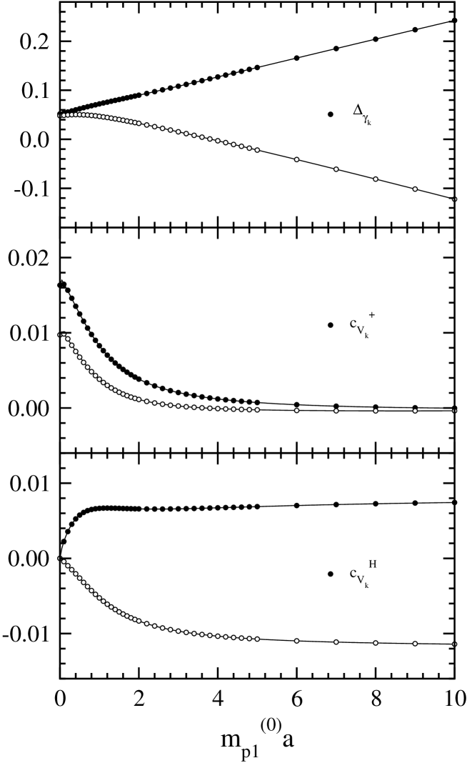
Figure 2: $\Delta_{\gamma_{k}},c_{V_{k}}^{(+,H)}$ for heavy-heavy case as a function of ${m_{p1}^{(0)}}$. Solid symbols denote the plaquette gauge action and open ones for the Iwasaki gauge action.

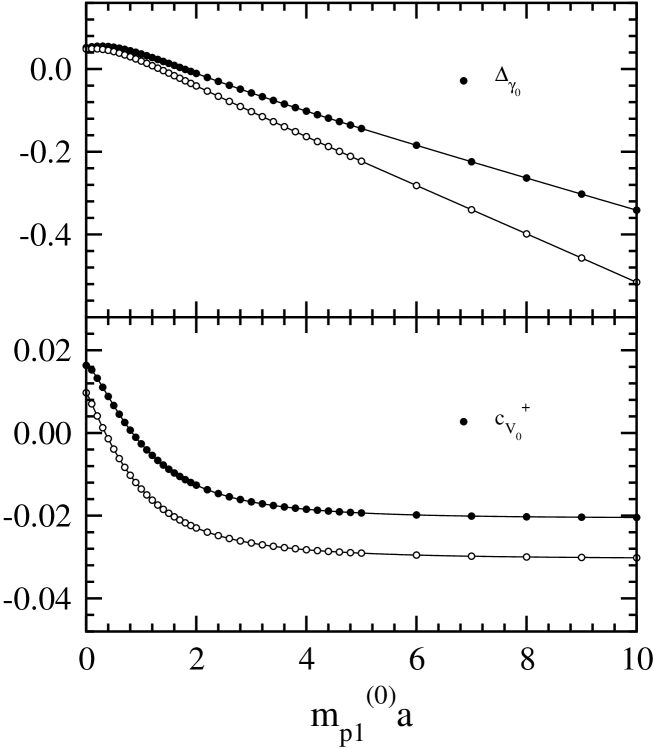
Figure 3: $\Delta_{\gamma_{0}},c_{V_{0}}^{+}$ for heavy-heavy case as a function of ${m_{p1}^{(0)}}$. Solid symbols denote the plaquette gauge action and open ones for the Iwasaki gauge action.

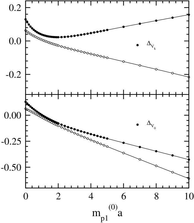
Figure 4: $\Delta_{V_{\mu}}$ for heavy-heavy case as a function of ${m_{p1}^{(0)}}$. Solid symbols denote the plaquette gauge action and open ones for the Iwasaki gauge action.

We obtain $\Delta_{\gamma_{k}},c_{V_{k}}^{(+,H)}$ and $\Delta_{\gamma_{0}},c_{V_{0}}^{+}$ from eqs.(17), (18) and (21$-$23) choosing ${m_{p1}}={m_{p2}}$, where the charge conjugation symmetry demands $c_{V_{k}}^{L}=c_{V_{k}}^{H}$ and $c_{V_{k}}^{-}=c_{V_{0}}^{-}=0$. In Figs. 2 and 3 we plot $\Delta_{\gamma_{k}},c_{V_{k}}^{(+,H)}$ and $\Delta_{\gamma_{0}},c_{V_{0}}^{+}$, respectively, as a function of ${m_{p1}^{(0)}}$ for the plaquette and the Iwasaki gauge actions. The ${m_{p1}^{(0)}}$ dependence of $\Delta_{V_{\mu}}$ in eq.(25) is also plotted in Fig. 4. The solid lines denote the fitting results of the interpolation:

$$\Delta_{\gamma_{k}} = \left.\Delta_{\gamma_{k}}\right|_{{m_{p1}^{(0)}}=0}+\frac{\sum_{i=1}^{5}v_{ni}^{k\gamma}\{{m_{p1}^{(0)}}\}^{i}}{1+\sum_{i=1}^{5}v_{di}^{k\gamma}\{{m_{p1}^{(0)}}\}^{i}},$$ (44)

$$c_{V_{k}}^{+} = \left.c_{V_{k}}^{+}\right|_{{m_{p1}^{(0)}}=0}+\frac{\sum_{i=1}^{5}v_{ni}^{k+}\{{m_{p1}^{(0)}}\}^{i}}{1+\sum_{i=1}^{5}v_{di}^{k+}\{{m_{p1}^{(0)}}\}^{i}},$$ (45)

$$c_{V_{k}}^{H} = \frac{\sum_{i=1}^{5}v_{ni}^{kH}\{{m_{p1}^{(0)}}\}^{i}}{1+\sum_{i=1}^{5}v_{di}^{kH}\{{m_{p1}^{(0)}}\}^{i}},$$ (46)

$$\Delta_{V_{k}} = \left.\Delta_{V_{k}}\right|_{{m_{p1}^{(0)}}=0}+\frac{\sum_{i=1}^{5}v_{ni}^{kZ}\{{m_{p1}^{(0)}}\}^{i}}{1+\sum_{i=1}^{5}v_{ni}^{kZ}\{{m_{p1}^{(0)}}\}^{i}},$$ (47)

$$\Delta_{\gamma_{0}} = \left.\Delta_{\gamma_{0}}\right|_{{m_{p1}^{(0)}}=0}+\frac{\sum_{i=1}^{5}v_{ni}^{0\gamma}\{{m_{p1}^{(0)}}\}^{i}}{1+\sum_{i=1}^{5}v_{di}^{0\gamma}\{{m_{p1}^{(0)}}\}^{i}},$$ (48)

$$c_{V_{0}}^{+} = \left.c_{V_{0}}^{+}\right|_{{m_{p1}^{(0)}}=0}+\frac{\sum_{i=1}^{5}v_{ni}^{0+}\{{m_{p1}^{(0)}}\}^{i}}{1+\sum_{i=1}^{5}v_{di}^{0+}\{{m_{p1}^{(0)}}\}^{i}},$$ (49)

$$\Delta_{V_{0}} = \left.\Delta_{V_{0}}\right|_{{m_{p1}^{(0)}}=0}+\frac{\sum_{i=1}^{5}v_{ni}^{0Z}\{{m_{p1}^{(0)}}\}^{i}}{1+\sum_{i=1}^{5}v_{di}^{0Z}\{{m_{p1}^{(0)}}\}^{i}},$$ (50)

where we assume $c_{V_{k}}^{H}=0$ at ${m_{p1}^{(0)}}=0$. We employ $\Delta_{\gamma_{k}}=\Delta_{\gamma_{0}}=$0.05169(plaqette), 0.04802(IwasakiIwasaki83 ), 0.04595(DBW2dbw2 ), $c_{V_{k}}^{+}=c_{V_{0}}^{+}=$0.01633(plaquette), 0.009728(Iwasaki), 0.004884(DBW2) and $\Delta_{V_{k}}=\Delta_{V_{0}}=$0.1294(plaquette), 0.06279(Iwasaki), 0.02566(DBW2) at ${m_{p1}^{(0)}}=0$. The values of the parameters $v_{ni}^{k,0}$ and $v_{di}^{k,0}$ ($i=1,\dots,5$) are summarized in Tables References and References. The relative errors of these interpolations to the data are less than a few % over the range $0\leq{m_{p1}^{(0)}}\leq 10$.

II.2.2 Heavy-light case

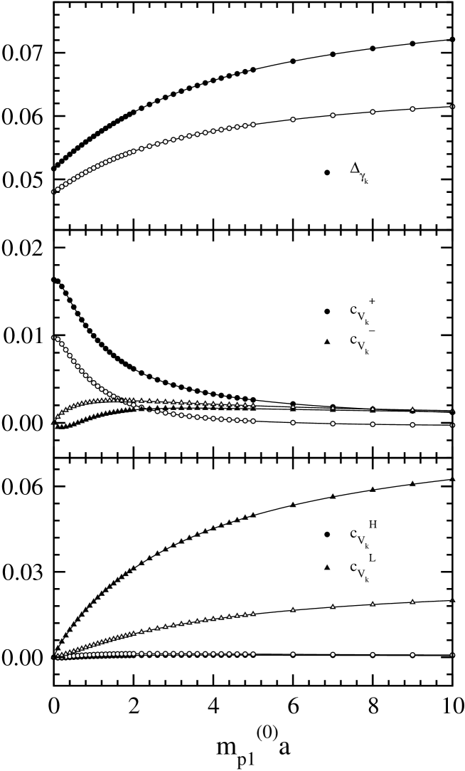
Figure 5: $\Delta_{\gamma_{k}},c_{V_{k}}^{(+,-,H,L)}$ for heavy-light case as a function of ${m_{p1}^{(0)}}$. Solid symbols denote the plaquette gauge action and open ones for the Iwasaki gauge action.

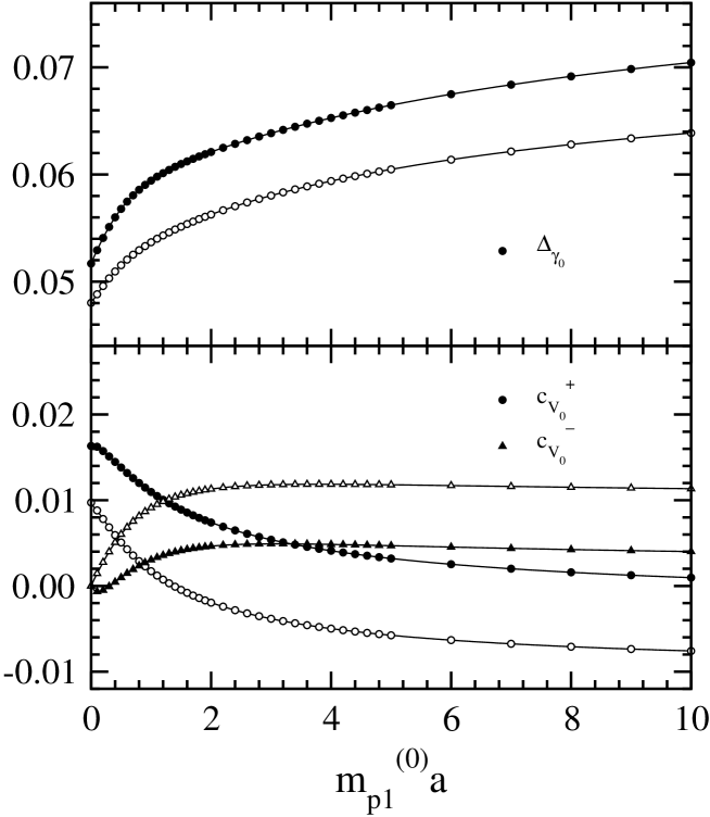
Figure 6: $\Delta_{\gamma_{0}},c_{V_{0}}^{(+,-)}$ for heavy-light case as a function of ${m_{p1}^{(0)}}$. Solid symbols denote the plaquette gauge action and open ones for the Iwasaki gauge action.

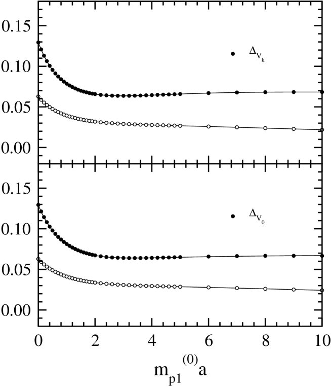
Figure 7: $\Delta_{V_{\mu}}$ for heavy-light case as a function of ${m_{p1}^{(0)}}$. Solid symbols denote the plaquette gauge action and open ones for the Iwasaki gauge action.

We use eqs.(17$-$24) to determine $\Delta_{\gamma_{k}}$, $c_{V_{k}}^{(+,-,H,L)}$ and $\Delta_{\gamma_{0}}$, $c_{V_{0}}^{(+,-)}$. Assuming that the ${m_{p2}}a$ corrections are negligible, we evaluate the improvement coefficients, except $c_{V_{k}}^{L}$ and $c_{V_{0}}^{(+,-)}$, as a function of ${m_{p1}^{(0)}}$ with ${m_{p2}^{(0)}}=0$. In eqs.(34), (36), (37) we find that $S_{k}^{s}$ and $Y_{0}^{d}-Z_{0}^{d}$ are not determined if we set ${m_{p2}^{(0)}}=0$. Therefore one should extrapolate data at non-zero ${m_{p2}^{(0)}}$ to ${m_{p2}^{(0)}}=0$. We however keep ${m_{p2}^{(0)}}=0.0001$ in our calculation to determine $c_{V_{k}}^{L}$ and $c_{V_{0}}^{(+,-)}$ since the difference between the value at ${m_{p2}^{(0)}}=0.0001$ and the one extrapolated to ${m_{p2}^{(0)}}=0$ is less than 1 %. Figures 5 and 6 show the ${m_{p1}^{(0)}}$ dependence of $\Delta_{\gamma_{k}}$, $c_{V_{k}}^{(+,-,H,L)}$ and $\Delta_{\gamma_{0}}$, $c_{V_{0}}^{(+,-)}$, respectively, for the plaquette and the Iwasaki gauge actions. We also plot $\Delta_{V_{\mu}}$ in Fig. 7. The interpolation denoted by the solid lines are expressed as

$$\Delta_{\gamma_{k}} = \left.\Delta_{\gamma_{k}}\right|_{{m_{p1}^{(0)}}=0}+\frac{\sum_{i=1}^{5}v_{ni}^{k\gamma}\{{m_{p1}^{(0)}}\}^{i}}{1+\sum_{i=1}^{5}v_{di}^{k\gamma}\{{m_{p1}^{(0)}}\}^{i}},$$ (51)

$$c_{V_{k}}^{+} = \left.c_{V_{k}}^{+}\right|_{{m_{p1}^{(0)}}=0}+\frac{\sum_{i=1}^{5}v_{ni}^{k+}\{{m_{p1}^{(0)}}\}^{i}}{1+\sum_{i=1}^{5}v_{di}^{k+}\{{m_{p1}^{(0)}}\}^{i}},$$ (52)

$$c_{V_{k}}^{(-,H,L)} = \frac{\sum_{i=1}^{5}v_{ni}^{k(-,H,L)}\{{m_{p1}^{(0)}}\}^{i}}{1+\sum_{i=1}^{5}v_{di}^{k(-,H,L)}\{{m_{p1}^{(0)}}\}^{i}},$$ (53)

$$\Delta_{V_{k}} = \left.\Delta_{V_{k}}\right|_{{m_{p1}^{(0)}}=0}+\frac{\sum_{i=1}^{5}v_{ni}^{kZ}\{{m_{p1}^{(0)}}\}^{i}}{1+\sum_{i=1}^{5}v_{di}^{kZ}\{{m_{p1}^{(0)}}\}^{i}},$$

$$\Delta_{\gamma_{0}} = \left.\Delta_{\gamma_{0}}\right|_{{m_{p1}^{(0)}}=0}+\frac{\sum_{i=1}^{5}v_{ni}^{0\gamma}\{{m_{p1}^{(0)}}\}^{i}}{1+\sum_{i=1}^{5}v_{di}^{0\gamma}\{{m_{p1}^{(0)}}\}^{i}},$$ (54)

$$c_{V_{0}}^{+} = \left.c_{V_{0}}^{+}\right|_{{m_{p1}^{(0)}}=0}+\frac{\sum_{i=1}^{5}v_{ni}^{0+}\{{m_{p1}^{(0)}}\}^{i}}{1+\sum_{i=1}^{5}v_{di}^{0+}\{{m_{p1}^{(0)}}\}^{i}},$$ (55)

$$c_{V_{0}}^{-} = \frac{\sum_{i=1}^{5}v_{ni}^{0-}\{{m_{p1}^{(0)}}\}^{i}}{1+\sum_{i=1}^{5}v_{di}^{0-}\{{m_{p1}^{(0)}}\}^{i}},$$ (56)

$$\Delta_{V_{0}} = \left.\Delta_{V_{0}}\right|_{{m_{p1}^{(0)}}=0}+\frac{\sum_{i=1}^{5}v_{ni}^{0Z}\{{m_{p1}^{(0)}}\}^{i}}{1+\sum_{i=1}^{5}v_{di}^{0Z}\{{m_{p1}^{(0)}}\}^{i}}$$ (57)

with $v_{ni}^{k,0}$ and $v_{di}^{k,0}$ ($i=1,\dots,5$) given in Tables References and References. Here we use the constraint that $c_{V_{k}}^{(-,H,L)}=0$ and $c_{V_{0}}^{-}=0$ at ${m_{p1}^{(0)}}=0$. The data are well described by these interpolations within a few % errors over the range $0\leq{m_{p1}^{(0)}}\leq 10$.

III $O(a)$ improvement of the axial vector currents

Let us turn to the axial vector currents. The discussion is in parallel with the case of the vector currents. The renormalized operators with the $O(a)$ improvement is given by

$$A^{{\rm latt},R}_{\mu}(x) = Z_{A}^{{\rm latt}}\left[{\bar{q}(x)}\gamma_{\mu}\gamma_{5}Q(x)-g^{2}c_{A_{\mu}}^{+}\partial_{\mu}^{+}\{{\bar{q}(x)}\gamma_{5}Q(x)\}-g^{2}c_{A_{\mu}}^{-}\partial_{\mu}^{-}\{{\bar{q}(x)}\gamma_{5}Q(x)\}\right.$$ (58)

$$\left.-g^{2}c_{A_{\mu}}^{L}\{{\vec{\partial}_{i}}{\bar{q}(x)}\}\gamma_{i}\gamma_{\mu}\gamma_{5}Q(x)-g^{2}c_{A_{\mu}}^{H}{\bar{q}(x)}\gamma_{\mu}\gamma_{5}\gamma_{i}\{{\vec{\partial}_{i}}Q(x)\}+O(g^{4})\right]\$$

where we assume that the Euclidean space-time rotational symmetry is not retained on the lattice. The coefficients $Z_{A_{\mu}}^{{\rm latt}}$ and $c_{A_{\mu}}^{(+,-,H,L)}$ are functions of the quark masses $m_{Q}$ and $m_{q}$. With the aid of equation of motion we are allowed to set $c^{H}_{A_{0}}=c^{L}_{A_{0}}=0$. In the special case of $m_{Q}=m_{q}$, $c_{A_{\mu}}^{-}=0$ and $c_{A_{\mu}}^{H}=c_{A_{\mu}}^{L}$ is derived from the charge conjugation symmetry. We also note that all the improvement coefficients except $c_{A_{\mu}}^{+}$ vanishes in the limit of $m_{Q}=m_{q}=0$. We determine $Z_{A_{\mu}}^{{\rm latt}}$ and $c_{A_{\mu}}^{(+,-,H,L)}$ at the one-loop level for both heavy-heavy and heavy-light cases.

III.1 Determination of the improvement coefficients for the axial vector currents

The general form of the off-shell vertex functions at the one-loop level on the lattice are given by

$$\Lambda_{k5}^{(1)}(p,q,{m_{p1}},{m_{p2}}) = \gamma_{k}\gamma_{5}F_{1}^{k5}+\gamma_{k}\gamma_{5}\{p\kern-4.30554pt/F_{2}^{k5}+p\kern-4.30554pt/_{s}F_{3}^{k5}\}+\{q\kern-4.30554pt/F_{4}^{k5+}q\kern-4.30554pt/_{s}F_{5}^{k5}\}\gamma_{k}\gamma_{5}$$ (59)

$$+q\kern-4.30554pt/\gamma_{k}\gamma_{5}p\kern-4.30554pt/F_{6}^{k5}+q\kern-4.30554pt/\gamma_{k}\gamma_{5}p\kern-4.30554pt/_{s}F_{7}^{k5}+q\kern-4.30554pt/_{s}\gamma_{k}\gamma_{5}p\kern-4.30554pt/F_{8}^{k5}+\gamma_{k}\gamma_{5}p\kern-4.30554pt/_{s}p\kern-4.30554pt/F_{9}^{k5}+q\kern-4.30554pt/q\kern-4.30554pt/_{s}\gamma_{k}\gamma_{5}F_{10}^{k5}$$

$$+(p_{k}-q_{k})\left[\gamma_{5}G_{1}^{k5}+\gamma_{5}p\kern-4.30554pt/G_{2}^{k5}+q\kern-4.30554pt/\gamma_{5}G_{3}^{k5}+q\kern-4.30554pt/\gamma_{5}p\kern-4.30554pt/G_{4}^{k5}\right]$$

$$+(p_{k}+q_{k})\left[\gamma_{5}H_{1}^{k5}+\gamma_{5}p\kern-4.30554pt/H_{2}^{k5}+q\kern-4.30554pt/\gamma_{5}H_{3}^{k5}+q\kern-4.30554pt/\gamma_{5}p\kern-4.30554pt/H_{4}^{k5}\right]+O(a^{2}),$$

$$\Lambda_{05}^{(1)}(p,q,{m_{p1}},{m_{p2}}) = \gamma_{0}\gamma_{5}F_{1}^{05}+\gamma_{0}\gamma_{5}p\kern-4.30554pt/F_{2}^{05}+q\kern-4.30554pt/\gamma_{0}\gamma_{5}F_{3}^{05}+q\kern-4.30554pt/\gamma_{0}\gamma_{5}p\kern-4.30554pt/F_{4}^{05}$$ (60)

$$+(p_{0}-q_{0})\left[\gamma_{5}G_{1}^{05}+\gamma_{5}p\kern-4.30554pt/G_{2}^{05}+q\kern-4.30554pt/\gamma_{5}G_{3}^{05}+q\kern-4.30554pt/\gamma_{5}p\kern-4.30554pt/G_{4}^{05}\right]$$

$$+(p_{0}+q_{0})\left[\gamma_{5}H_{1}^{05}+\gamma_{5}p\kern-4.30554pt/H_{2}^{05}+q\kern-4.30554pt/\gamma_{5}H_{3}^{05}+q\kern-4.30554pt/\gamma_{5}p\kern-4.30554pt/H_{4}^{05}\right]+O(a^{2}),$$

where the coefficients $F^{\mu 5}$, $G^{\mu 5}$, $H^{\mu 5}$ are functions of $p^{2}$, $q^{2}$, $p\cdot q$, ${m_{p1}}$ and ${m_{p2}}$.

Sandwiching (59) and (60) by the on-shell quark states $u(p)$ and $\bar{u}(q)$, which satisfy $p\kern-4.30554pt/u(p)=i{m_{p1}}u(p)$ and $\bar{u}(q)q\kern-4.30554pt/=i{m_{p2}}\bar{u}(q)$, the matrix elements are reduced to

$${\bar{u}}(q)\Lambda_{k5}^{(1)}(p,q,{m_{p1}},{m_{p2}})u(p)$$ (61)

$$= {\bar{u}}(q)\gamma_{k}\gamma_{5}u(p)\left\{F_{1}^{k5}+i{m_{p1}}F_{2}^{k5}+i{m_{p2}}F_{4}^{k5}-{m_{p1}}{m_{p2}}F_{6}^{k5}\right\}$$

$$+{\bar{u}}(q)\gamma_{k}\gamma_{5}p\kern-4.30554pt/_{s}u(p)\left\{F_{3}^{k5}+i{m_{p2}}F_{7}^{k5}+i{m_{p1}}F_{9}^{k5}\right\}$$

$$+{\bar{u}}(q)q\kern-4.30554pt/_{s}\gamma_{k}\gamma_{5}u(p)\left\{F_{5}^{k5}+i{m_{p1}}F_{8}^{k5}+i{m_{p2}}F_{10}^{k5}\right\}$$

$$+(p_{k}-q_{k}){\bar{u}}(q)\gamma_{5}u(p)\left\{G_{1}^{k5}+i{m_{p1}}G_{2}^{k5}+i{m_{p2}}G_{3}^{k5}-{m_{p1}}{m_{p2}}G_{4}^{k5}\right\}$$

$$+(p_{k}+q_{k}){\bar{u}}(q)\gamma_{5}u(p)\left\{H_{1}^{k5}+i{m_{p1}}H_{2}^{k5}+i{m_{p2}}H_{3}^{k5}-{m_{p1}}{m_{p2}}H_{4}^{k5}\right\}+O(a^{2}),$$

and

$${\bar{u}}(q)\Lambda_{05}^{(1)}(p,q,{m_{p1}},{m_{p2}})u(p)$$ (62)

$$= {\bar{u}}(q)\gamma_{0}\gamma_{5}u(p)\left\{F_{1}^{05}+i{m_{p1}}F_{2}^{05}+i{m_{p2}}F_{3}^{05}-{m_{p1}}{m_{p2}}F_{4}^{05}\right\}$$

$$+(p_{0}-q_{0}){\bar{u}}(q)u(p)\left\{G_{1}^{05}+i{m_{p1}}G_{2}^{05}+i{m_{p2}}G_{3}^{05}-{m_{p1}}{m_{p2}}G_{4}^{05}\right\}$$

$$+(p_{0}+q_{0}){\bar{u}}(q)\gamma_{5}u(p)\left\{H_{1}^{05}+i{m_{p1}}H_{2}^{05}+i{m_{p2}}H_{3}^{05}-{m_{p1}}{m_{p2}}H_{4}^{05}\right\}+O(a^{2}),$$

where the coefficients are summarized as

$$X_{k5} = F_{1}^{k5}+i{m_{p1}}F_{2}^{k5}+i{m_{p2}}F_{4}^{k5}-{m_{p1}}{m_{p2}}F_{6}^{k5},$$ (63)

$$Y_{k5} = G_{1}^{k5}+i{m_{p1}}G_{2}^{k5}+i{m_{p2}}G_{3}^{k5}-{m_{p1}}{m_{p2}}G_{4}^{k5},$$ (64)

$$Z_{k5} = H_{1}^{k5}+i{m_{p1}}H_{2}^{k5}+i{m_{p2}}H_{3}^{k5}-{m_{p1}}{m_{p2}}H_{4}^{k5},$$ (65)

$$R_{k5} = F_{3}^{k5}+i{m_{p2}}F_{7}^{k5}+i{m_{p1}}F_{9}^{k5},$$ (66)

$$S_{k5} = F_{5}^{k5}+i{m_{p1}}F_{8}^{k5}+i{m_{p2}}F_{10}^{k5}$$ (67)

and

$$X_{05} = F_{1}^{05}+i{m_{p1}}F_{2}^{05}+i{m_{p2}}F_{3}^{05}-{m_{p1}}{m_{p2}}F_{4}^{05},$$ (68)

$$Y_{05} = G_{1}^{05}+i{m_{p1}}G_{2}^{05}+i{m_{p2}}G_{3}^{05}-{m_{p1}}{m_{p2}}G_{4}^{05},$$ (69)

$$Z_{05} = H_{1}^{05}+i{m_{p1}}H_{2}^{05}+i{m_{p2}}H_{3}^{05}-{m_{p1}}{m_{p2}}H_{4}^{05}.$$ (70)

In terms of these coefficients the improvement coefficients in eq.(58) are given by

$$\Delta_{\gamma_{k}\gamma_{5}} = \left(X_{k5}\right)^{\rm latt}-\left(X_{k5}\right)^{\rm cont},$$ (71)

$$ic_{A_{k}}^{+} = \left(Y_{k5}\right)^{\rm latt}-\left(Y_{k5}\right)^{\rm cont},$$ (72)

$$ic_{A_{k}}^{-} = \left(Z_{k5}\right)^{\rm latt}-\left(Z_{k5}\right)^{\rm cont},$$ (73)

$$-ic_{A_{k}}^{L} = \left(S_{k5}\right)^{\rm latt},$$ (74)

$$ic_{A_{k}}^{H} = \left(R_{k5}\right)^{\rm latt},$$ (75)

$$\Delta_{\gamma_{0}\gamma_{5}} = \left(X_{05}\right)^{\rm latt}-\left(X_{05}\right)^{\rm cont},$$ (76)

$$ic_{A_{0}}^{+} = \left(Y_{05}\right)^{\rm latt}-\left(Y_{05}\right)^{\rm cont},$$ (77)

$$ic_{A_{0}}^{-} = \left(Z_{05}\right)^{\rm latt}-\left(Z_{05}\right)^{\rm cont},$$ (78)

where we calculate the continuum contributions employing the ${\overline{\rm MS}}$ scheme with NDR. It should be noted that $R_{k5}=S_{k5}=0$ in the continuum from the space-time rotational symmetry and $c_{A_{k}}^{L}=c_{A_{k}}^{H}$ and $c_{A_{k}}^{-}=c_{A_{0}}^{-}=0$ for ${m_{p1}}={m_{p2}}$ from the charge conjugation symmetry.

Combining $\Delta_{\gamma_{\mu}\gamma_{5}}$ and the wave function renormalization factors, we obtain the renormalization factor of the axial vector currents:

$$\frac{Z_{A_{\mu}}^{\rm latt}}{Z_{A_{\mu}}^{\rm cont}}=\sqrt{Z_{Q,{\rm latt}}^{(0)}({m_{p1}^{(0)}})}\sqrt{Z_{q,{\rm latt}}^{(0)}({m_{p2}^{(0)}})}\left(1-g^{2}\Delta_{A_{\mu}}\right)$$ (79)

with

$$Z_{Q,{\rm latt}}^{(0)}({m_{p1}^{(0)}}) = \cosh({m_{p1}^{(0)}})+r_{t}\sinh({m_{p1}^{(0)}})$$ (80)

$$Z_{q,{\rm latt}}^{(0)}({m_{p2}^{(0)}}) = \cosh({m_{p2}^{(0)}})+r_{t}\sinh({m_{p2}^{(0)}})$$ (81)

$$\Delta_{A_{\mu}} = \Delta_{\gamma_{\mu}\gamma_{5}}-\frac{\Delta_{Q}}{2}-\frac{\Delta_{q}}{2},$$ (82)

where $\Delta_{Q,q}$ are found in Ref. param . For convenience we give the relation for $Z_{A_{\mu}}^{\rm cont}$ between NDR and DRED in ${\overline{\rm MS}}$ scheme:

$$Z_{A_{\mu}}^{\rm cont}({\rm NDR})=Z_{A_{\mu}}^{\rm cont}({\rm DRED})-\frac{1}{2}g^{2}.$$ (83)

The relevant coefficients $X_{k5},Y_{k5},Z_{k5},R_{k5},S_{k5}$ for $A_{k}$ are determined from the off-shell vertex function (59):

$$X_{k5}^{s} = \frac{1}{4}{\rm Tr}\left[\Lambda_{k5}^{(1)}(1+\gamma_{0})\gamma_{5}\gamma_{k}\right]_{p={p^{*}},q={q^{*}_{s}}},$$ (84)

$$Y_{k5}^{d}+Z_{k5}^{d} = \frac{1}{4}{\rm Tr}\left[\frac{\partial}{\partial p_{k}}\Lambda_{k5}^{(1)}(1+\gamma_{0})\gamma_{5}-\frac{\partial}{\partial p_{i}}\Lambda_{k5}^{(1)}(1+\gamma_{0})\gamma_{i}\gamma_{k}\gamma_{5}\right]^{i\neq k}_{p={p^{*}},q={q^{*}_{d}}},$$ (85)

$$Y_{k5}^{d}-Z_{k5}^{d} = \frac{1}{4}{\rm Tr}\left[-\frac{\partial}{\partial q_{k}}\Lambda_{k5}^{(1)}(1+\gamma_{0})\gamma_{5}+\frac{\partial}{\partial q_{i}}\Lambda_{k5}^{(1)}(1+\gamma_{0})\gamma_{k}\gamma_{i}\gamma_{5}\right]^{i\neq k}_{p={p^{*}},q={q^{*}_{d}}},$$ (86)

$$X_{k5}^{d}+2i{m_{p1}}R_{k5}^{d} = \frac{1}{4}{\rm Tr}\left[\Lambda_{k5}^{(1)}\gamma_{5}\gamma_{k}(1-\gamma_{0})+2i{m_{p1}}\frac{\partial}{\partial p_{i}}\Lambda_{k}^{(1)}(1+\gamma_{0})\gamma_{i}\gamma_{5}\gamma_{k}\right]^{i\neq k}_{p={p^{*}},q={q^{*}_{d}}},$$ (87)

$$X_{k5}^{d}+2i{m_{p2}}S_{k5}^{d} = \frac{1}{4}{\rm Tr}\left[\Lambda_{k}^{(1)}(1+\gamma_{0})\gamma_{5}\gamma_{k}+2i{m_{p2}}\frac{\partial}{\partial q_{i}}\Lambda_{k}^{(1)}(1+\gamma_{0})\gamma_{5}\gamma_{k}\gamma_{i}\right]^{i\neq k}_{p={p^{*}},q={q^{*}_{d}}},$$ (88)

where ${p^{*}}\equiv(p_{0}=im_{p1},p_{i}=0)$ and ${q^{*}_{s}}\equiv(q_{0}=im_{p2},q_{i}=0)$ or ${q^{*}_{d}}\equiv(q_{0}=-im_{p2},q_{i}=0)$. We obtain $X_{05},Y_{05},Z_{05}$ for $A_{0}$ from eq.(60):

$$X_{05}^{s}$$

$$=\frac{1}{4}{\rm Tr}\left[\Lambda_{05}^{(1)}\gamma_{5}\gamma_{0}+i{m_{p1}}\frac{\partial}{\partial p_{k}}\Lambda_{05}^{(1)}(1+\gamma_{0})\gamma_{k}\gamma_{5}+i{m_{p2}}\frac{\partial}{\partial q_{k}}\Lambda_{05}^{(1)}(1+\gamma_{0})\gamma_{k}\gamma_{5}\right]_{p={p^{*}},q={q^{*}_{s}}},$$ (89)

$$X_{05}^{s}+i{m_{p1}}(Y_{05}^{s}+Z_{05}^{s})-i{m_{p2}}(Y_{05}^{s}-Z_{05}^{s})$$

$$=\frac{1}{4}{\rm Tr}\left[\Lambda_{05}^{(1)}\gamma_{5}(1+\gamma_{0})+2i{m_{p1}}\frac{\partial}{\partial p_{k}}\Lambda_{05}^{(1)}(1+\gamma_{0})\gamma_{k}\gamma_{5}\right]_{p={p^{*}},q={q^{*}_{s}}},$$ (90)

$$X_{05}^{d}-i{m_{p1}}(Y_{05}^{d}+Z_{05}^{d})-i{m_{p2}}(Y_{05}^{d}-Z_{05}^{d})=-\frac{1}{4}{\rm Tr}\left[\Lambda_{05}^{(1)}(1+\gamma_{0})\gamma_{5}\right]_{p={p^{*}},q={q^{*}_{d}}},$$ (91)

where $F^{k}$, $G^{k}$ and $H^{k}$ are functions of $p^{2}$, $q^{2}$ and $p\cdot q$ resulting in

$$\left.\frac{\partial F^{\mu 5}}{\partial p_{i}}\right|_{p={p^{*}},q={q^{*}}}=\left.\frac{\partial F^{\mu 5}}{\partial q_{i}}\right|_{p={p^{*}},q={q^{*}}}=0,$$ (92)

$$\left.\frac{\partial H^{\mu 5}}{\partial p_{i}}\right|_{p={p^{*}},q={q^{*}}}=\left.\frac{\partial H^{\mu 5}}{\partial q_{i}}\right|_{p={p^{*}},q={q^{*}}}=0,$$ (93)

$$\left.\frac{\partial G^{\mu 5}}{\partial p_{i}}\right|_{p={p^{*}},q={q^{*}}}=\left.\frac{\partial G^{\mu 5}}{\partial q_{i}}\right|_{p={p^{*}},q={q^{*}}}=0$$ (94)

with $i=1,2,3$.

As for the counterterm to isolate the infrared divergence in the above coefficients at the one-loop level we employ

$${\tilde{I}}_{\mu 5}(k,p,q,{m_{p1}^{(0)}},{m_{p2}^{(0)}},\lambda)$$ (95)

$$= \theta(\Lambda^{2}-k^{2})C_{F}i\gamma_{\alpha}\frac{1}{i(q\kern-4.30554pt/+k\kern-4.30554pt/)+{m_{p2}^{(0)}}}\gamma_{\mu}\gamma_{5}\frac{1}{i(p\kern-4.30554pt/+k\kern-4.30554pt/)+{m_{p1}^{(0)}}}i\gamma_{\alpha}\frac{1}{k^{2}+\lambda^{2}}$$

with a cutoff $\Lambda$ $(\leq\pi)$.

III.2 Results for the improvement coefficients of the axial vector currents

III.2.1 Heavy-heavy case

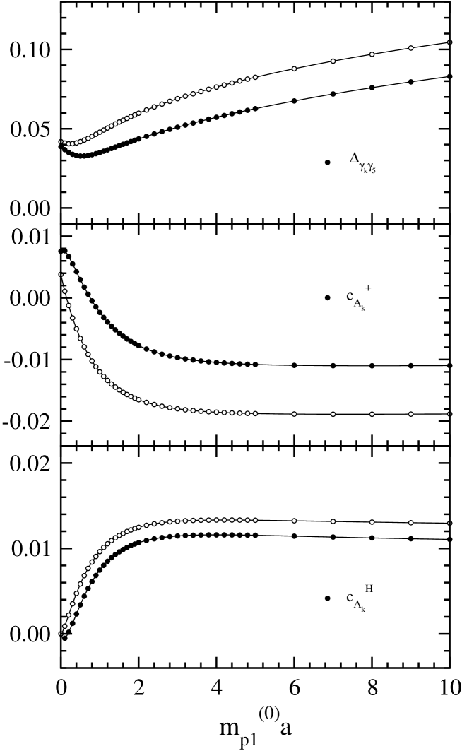
Figure 8: $\Delta_{\gamma_{k}\gamma_{5}},c_{A_{k}}^{(+,H)}$ for heavy-heavy case as a function of ${m_{p1}^{(0)}}$. Solid symbols denote the plaquette gauge action and open ones for the Iwasaki gauge action.

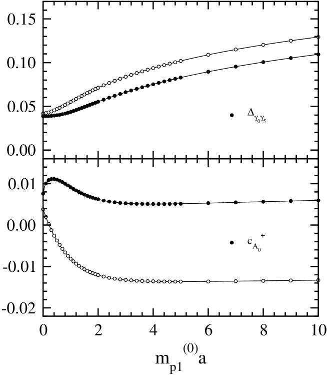
Figure 9: $\Delta_{\gamma_{0}\gamma_{5}},c_{A_{0}}^{+}$ for heavy-heavy case as a function of ${m_{p1}^{(0)}}$. Solid symbols denote the plaquette gauge action and open ones for the Iwasaki gauge action.

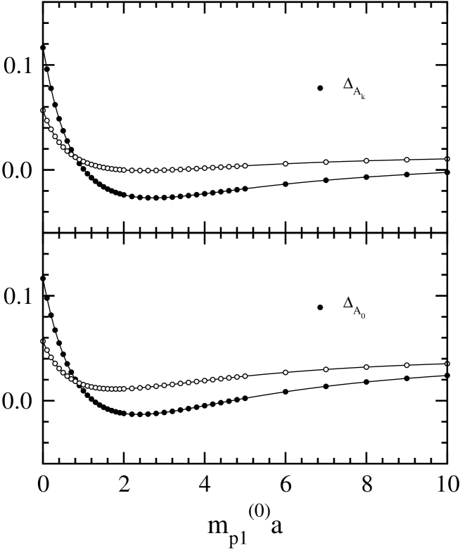
Figure 10: $\Delta_{A_{\mu}}$ for heavy-heavy case as a function of ${m_{p1}^{(0)}}$. Solid symbols denote the plaquette gauge action and open ones for the Iwasaki gauge action.

With the choice of ${m_{p1}}={m_{p2}}$ the improvement coefficients $\Delta_{\gamma_{k}\gamma_{5}},c_{A_{k}}^{(+,H)}$ and $\Delta_{\gamma_{0}\gamma_{5}},c_{A_{0}}^{+}$ are determined from eqs.(71), (72) and (75$-$77). It is noted that $c_{A_{k}}^{L}=c_{A_{k}}^{H}$ and $c_{A_{k}}^{-}=c_{A_{0}}^{-}=0$ from the charge conjugation symmetry. The quark mass dependences of $\Delta_{\gamma_{k}\gamma_{5}},c_{A_{k}}^{(+,H)}$ and $\Delta_{\gamma_{0}\gamma_{5}},c_{A_{0}}^{+}$ are shown in Figs. 8 and 9, respectively, employing the plaquette and the Iwasaki gauge actions. We also give the ${m_{p1}^{(0)}}$ dependence of $\Delta_{A_{\mu}}$ in Fig. 10. The solid lines denote the interpolation with the use of the following functions:

$$\Delta_{\gamma_{k}\gamma_{5}} = \left.\Delta_{\gamma_{k}\gamma_{5}}\right|_{{m_{p1}^{(0)}}=0}+\frac{\sum_{i=1}^{5}a_{ni}^{k\gamma}\{{m_{p1}^{(0)}}\}^{i}}{1+\sum_{i=1}^{5}a_{di}^{k\gamma}\{{m_{p1}^{(0)}}\}^{i}},$$ (96)

$$c_{A_{k}}^{+} = \left.c_{A_{k}}^{+}\right|_{{m_{p1}^{(0)}}=0}+\frac{\sum_{i=1}^{5}a_{ni}^{k+}\{{m_{p1}^{(0)}}\}^{i}}{1+\sum_{i=1}^{5}a_{di}^{k+}\{{m_{p1}^{(0)}}\}^{i}},$$ (97)

$$c_{A_{k}}^{H} = \frac{\sum_{i=1}^{5}a_{ni}^{kH}\{{m_{p1}^{(0)}}\}^{i}}{1+\sum_{i=1}^{5}a_{di}^{k+}\{{m_{p1}^{(0)}}\}^{i}},$$ (98)

$$\Delta_{A_{k}} = \left.\Delta_{A_{k}}\right|_{{m_{p1}^{(0)}}=0}+\frac{\sum_{i=1}^{5}a_{ni}^{kZ}\{{m_{p1}^{(0)}}\}^{i}}{1+\sum_{i=1}^{5}a_{ni}^{kZ}\{{m_{p1}^{(0)}}\}^{i}},$$ (99)

$$\Delta_{\gamma_{0}\gamma_{5}} = \left.\Delta_{\gamma_{0}\gamma_{5}}\right|_{{m_{p1}^{(0)}}=0}+\frac{\sum_{i=1}^{5}a_{ni}^{0\gamma}\{{m_{p1}^{(0)}}\}^{i}}{1+\sum_{i=1}^{5}a_{di}^{0\gamma}\{{m_{p1}^{(0)}}\}^{i}},$$ (100)

$$c_{A_{0}}^{+} = \left.c_{A_{0}}^{+}\right|_{{m_{p1}^{(0)}}=0}+\frac{\sum_{i=1}^{5}a_{ni}^{0+}\{{m_{p1}^{(0)}}\}^{i}}{1+\sum_{i=1}^{5}a_{di}^{0+}\{{m_{p1}^{(0)}}\}^{i}},$$ (101)

$$\Delta_{A_{0}} = \left.\Delta_{A_{0}}\right|_{{m_{p1}^{(0)}}=0}+\frac{\sum_{i=1}^{5}a_{ni}^{0Z}\{{m_{p1}^{(0)}}\}^{i}}{1+\sum_{i=1}^{5}a_{di}^{0Z}\{{m_{p1}^{(0)}}\}^{i}},$$ (102)

with $a_{ni}^{k,0}$ and $a_{di}^{k,0}$ ($i=1,\dots,5$) given in Tables References and References. The relative errors of these interpolations are a few % over the range $0\leq{m_{p1}^{(0)}}\leq 10$. The massless values are $\Delta_{\gamma_{k}\gamma_{5}}=\Delta_{\gamma_{0}\gamma_{5}}=$0.03873(plaqette), 0.04184(Iwasaki), 0.04359(DBW2), $c_{A_{k}}^{+}=c_{A_{0}}^{+}=$0.007574(plaquette), 0.003801(Iwasaki), 0.001492(DBW2) and $\Delta_{A_{k}}=\Delta_{A_{0}}=$0.1165(plaquette), 0.05663(Iwasaki), 0.02330(DBW2). The coefficient $c_{A_{k}}^{H}$ should vanish at ${m_{p1}^{(0)}}=0$.

III.2.2 Heavy-light case

The set of improvement coefficients are determined from eqs.(71$-$78). For the same reason before we keep ${m_{p2}^{(0)}}=0.0001$ for the determination of $c_{A_{k}}^{L}$ and $c_{A_{0}}^{(+,-)}$, while the vanishing light quark mass ${m_{p2}^{(0)}}=0$ is employed for other coefficients.

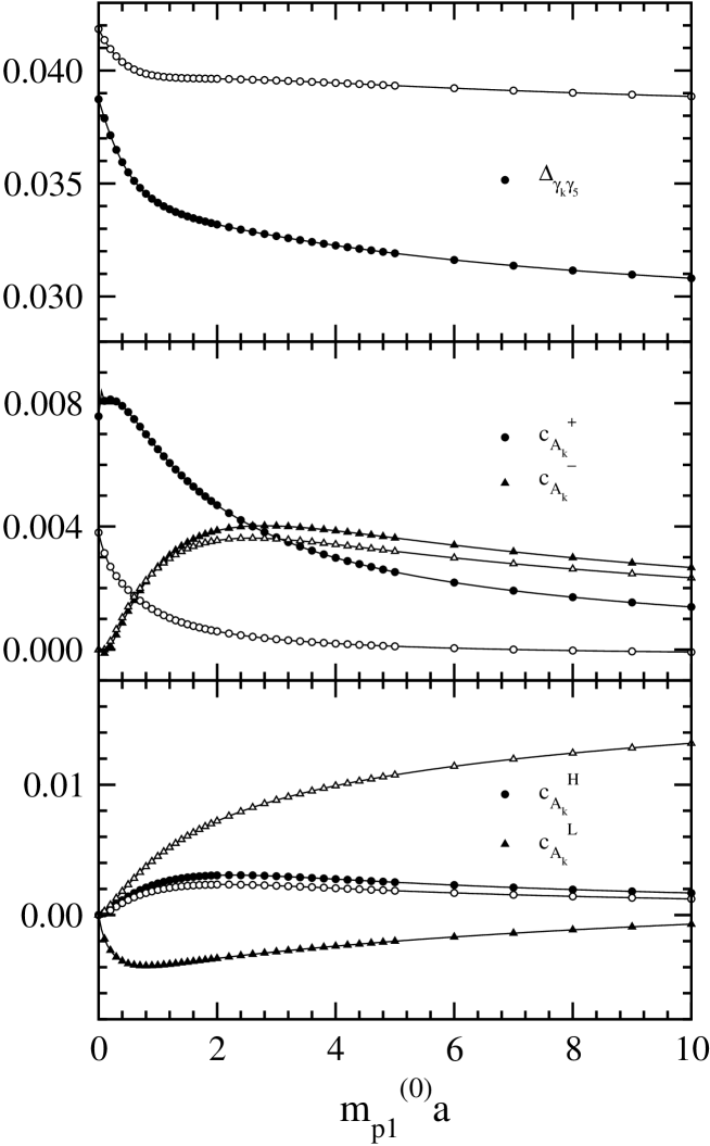
Figure 11: $\Delta_{\gamma_{k}\gamma_{5}},c_{A_{k}}^{(+,-,H,L)}$ for heavy-light case as a function of ${m_{p1}^{(0)}}$. Solid symbols denote the plaquette gauge action and open ones for the Iwasaki gauge action.

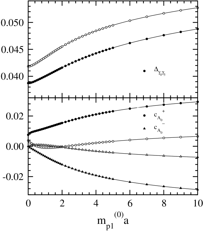
Figure 12: $\Delta_{\gamma_{0}\gamma_{5}},c_{A_{0}}^{(+,-)}$ for heavy-light case as a function of ${m_{p1}^{(0)}}$. Solid symbols denote the plaquette gauge action and open ones for the Iwasaki gauge action.

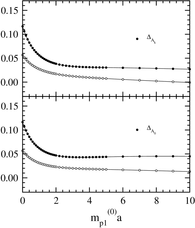
Figure 13: $\Delta_{A_{\mu}}$ for heavy-light case as a function of ${m_{p1}^{(0)}}$. Solid symbols denote the plaquette gauge action and open ones for the Iwasaki gauge action.

Numerical results for $\Delta_{\gamma_{k}\gamma_{5}}$, $c_{A_{k}}^{(+,-,H,L)}$ and $\Delta_{\gamma_{0}\gamma_{5}}$, $c_{A_{0}}^{(+,-)}$ are presented in Figs. 11 and 12 respectively, in the case of the plaquette and the Iwasaki gauge actions. We also plot the ${m_{p1}^{(0)}}$ dependence of $\Delta_{A_{\mu}}$ in Fig. 13. The solid lines represent the interpolation expressed as

$$\Delta_{\gamma_{k}\gamma_{5}} = \left.\Delta_{\gamma_{k}\gamma_{5}}\right|_{{m_{p1}^{(0)}}=0}+\frac{\sum_{i=1}^{5}a_{ni}^{k\gamma}\{{m_{p1}^{(0)}}\}^{i}}{1+\sum_{i=1}^{5}a_{di}^{k\gamma}\{{m_{p1}^{(0)}}\}^{i}},$$ (103)

$$c_{A_{k}}^{+} = \left.c_{A_{k}}^{+}\right|_{{m_{p1}^{(0)}}=0}+\frac{\sum_{i=1}^{5}a_{ni}^{k+}\{{m_{p1}^{(0)}}\}^{i}}{1+\sum_{i=1}^{5}a_{di}^{k+}\{{m_{p1}^{(0)}}\}^{i}},$$ (104)

$$c_{A_{k}}^{(-,H,L)} = \frac{\sum_{i=1}^{5}a_{ni}^{k(-,H,L)}\{{m_{p1}^{(0)}}\}^{i}}{1+\sum_{i=1}^{5}a_{di}^{k(-,H,L)}\{{m_{p1}^{(0)}}\}^{i}},$$ (105)

$$\Delta_{A_{k}} = \left.\Delta_{A_{k}}\right|_{{m_{p1}^{(0)}}=0}+\frac{\sum_{i=1}^{5}a_{di}^{kZ}\{{m_{p1}^{(0)}}\}^{i}}{1+\sum_{i=1}^{5}a_{di}^{kZ}\{{m_{p1}^{(0)}}\}^{i}},$$

$$\Delta_{\gamma_{0}\gamma_{5}} = \left.\Delta_{\gamma_{0}\gamma_{5}}\right|_{{m_{p1}^{(0)}}=0}+\frac{\sum_{i=1}^{5}a_{ni}^{0\gamma}\{{m_{p1}^{(0)}}\}^{i}}{1+\sum_{i=1}^{5}a_{di}^{0\gamma}\{{m_{p1}^{(0)}}\}^{i}},$$ (106)

$$c_{A_{0}}^{+} = \left.c_{A_{0}}^{+}\right|_{{m_{p1}^{(0)}}=0}+\frac{\sum_{i=1}^{5}a_{ni}^{0+}\{{m_{p1}^{(0)}}\}^{i}}{1+\sum_{i=1}^{5}a_{di}^{0+}\{{m_{p1}^{(0)}}\}^{i}},$$ (107)

$$c_{A_{0}}^{-} = \frac{\sum_{i=1}^{5}a_{ni}^{0-}\{{m_{p1}^{(0)}}\}^{i}}{1+\sum_{i=1}^{5}a_{di}^{0-}\{{m_{p1}^{(0)}}\}^{i}},$$ (108)

$$\Delta_{A_{0}} = \left.\Delta_{A_{0}}\right|_{{m_{p1}^{(0)}}=0}+\frac{\sum_{i=1}^{5}a_{ni}^{0Z}\{{m_{p1}^{(0)}}\}^{i}}{1+\sum_{i=1}^{5}a_{di}^{0Z}\{{m_{p1}^{(0)}}\}^{i}},$$ (109)

where the relative errors to the data are a few % over the range $0\leq{m_{p1}^{(0)}}\leq 10$. The values of the parameters $a_{ni}^{k,0}$ and $a_{di}^{k,0}$ ($i=1,\dots,5$) are listed in Table References and References. Here we use the constraint that $c_{A_{k}}^{(-,H,L)}$ and $c_{A_{0}}^{(-)}$ vanish at ${m_{p1}^{(0)}}=0$.

IV Mean field improvement

Let us explain the mean-field improvement on the renormalization factors of the vector and the axial vector currents in eqs.(25) and (79). We first rewritten their expressions as follows:

$$\frac{Z_{V_{\mu}}^{\rm latt}}{Z_{V_{\mu}}^{\rm cont}} = \sqrt{Z_{Q,{\rm latt}}^{(0)}({{\tilde{m}_{p1}}^{(0)}})}\sqrt{Z_{q,{\rm latt}}^{(0)}({{\tilde{m}_{p2}}^{(0)}})}u\left(1-g^{2}\Delta_{V_{\mu}}\right.$$ (110)

$$\left.+g^{2}\frac{C_{F}}{2}T_{\rm MF}+\frac{1}{2}\frac{g^{2}}{Z_{Q,{\rm latt}}^{(0)}}\frac{\partial Z_{Q,{\rm latt}}^{(0)}}{\partial{m_{p1}^{(0)}}}{\Delta{m_{p1}}}+\frac{1}{2}\frac{g^{2}}{Z_{q,{\rm latt}}^{(0)}}\frac{\partial Z_{q,{\rm latt}}^{(0)}}{\partial{m_{p2}^{(0)}}}{\Delta{m_{p2}}}\right),$$

$$\frac{Z_{A_{\mu}}^{\rm latt}}{Z_{A_{\mu}}^{\rm cont}} = \sqrt{Z_{Q,{\rm latt}}^{(0)}({{\tilde{m}_{p1}}^{(0)}})}\sqrt{Z_{q,{\rm latt}}^{(0)}({{\tilde{m}_{p2}}^{(0)}})}u\left(1-g^{2}\Delta_{A_{\mu}}\right.$$ (111)

$$\left.+g^{2}\frac{C_{F}}{2}T_{\rm MF}+\frac{1}{2}\frac{g^{2}}{Z_{Q,{\rm latt}}^{(0)}}\frac{\partial Z_{Q,{\rm latt}}^{(0)}}{\partial{m_{p1}^{(0)}}}{\Delta{m_{p1}}}+\frac{1}{2}\frac{g^{2}}{Z_{q,{\rm latt}}^{(0)}}\frac{\partial Z_{q,{\rm latt}}^{(0)}}{\partial{m_{p2}^{(0)}}}{\Delta{m_{p2}}}\right),$$

where ${\tilde{m}_{p1,2}}^{(0)}$ and $\Delta m_{p1,2}$ are defined in Ref. param and $T_{\rm MF}$ is the one-loop correction to the mean-field factor defined by

$$u=P^{1/4}=1-g^{2}\frac{C_{F}}{2}T_{\rm MF}$$ (112)

with $P$ the plaquette. We find a detailed description on the derivation of $T_{\rm MF}$ in Sec. III of Ref. dwf_pt_rg . We then replace $u$ by $P^{1/4}$ measured by Monte Carlo simulation.

The mean-field improved ${\overline{\rm MS}}$ coupling $g_{\overline{\rm MS}}^{2}(\mu)$ at the scale $\mu$ is obtained using the lattice bare coupling $g_{0}^{2}$ and $P$:

$$\displaystyle\frac{1}{g_{\overline{\rm MS}}^{2}(\mu)} = \displaystyle\frac{P}{g^{2}_{0}}+d_{g}+c_{p}+\displaystyle\frac{22}{16\pi^{2}}\log(\mu a)+N_{f}\left(d_{f}-\displaystyle\frac{4}{48\pi^{2}}\log(\mu a)\right)$$ (113)

with $N_{f}$ the number of quark flavor. The values of $c_{p}$, $d_{g}$ and $d_{f}$ for various gauge and quark actions are summarized in Ref. lambda_dwf . For the improved gauge action one may use an alternative formulacppacs

$$\displaystyle\frac{1}{g_{\overline{\rm MS}}^{2}(\mu)} = \displaystyle\frac{c_{0}P+8c_{1}R1+16c_{2}R2+8c_{3}R3}{g^{2}_{0}}$$ (114)

$$+d_{g}+(c_{0}\cdot c_{p}+8c_{1}\cdot c_{R1}+16c_{2}\cdot c_{R2}+8c_{3}\cdot c_{R3})+\displaystyle\frac{22}{16\pi^{2}}\log(\mu a)$$

$$+N_{f}\left(d_{f}-\displaystyle\frac{4}{48\pi^{2}}\log(\mu a)\right),$$

where

$$P = \frac{1}{3}{\rm Tr}U_{pl}=1-c_{p}g_{0}^{2}+O(g_{0}^{4}),$$ (115)

$$R1 = \frac{1}{3}{\rm Tr}U_{rtg}=1-c_{R1}g_{0}^{2}+O(g_{0}^{4}),$$ (116)

$$R2 = \frac{1}{3}{\rm Tr}U_{chr}=1-c_{R2}g_{0}^{2}+O(g_{0}^{4}),$$ (117)

$$R3 = \frac{1}{3}{\rm Tr}U_{plg}=1-c_{R3}g_{0}^{2}+O(g_{0}^{4}),$$ (118)

and the measured values are employed for $P$, $R1$, $R2$ and $R3$. We also find the values of $c_{R1}$, $c_{R2}$ and $c_{R3}$ for various gauge actions in Ref. lambda_dwf .

V Conclusion

In this paper we have determined the $O(a)$ improvement coefficients of the vector and the axial vector currents in a mass dependent way at the one-loop level. Our calculation is made employing the relativistic heavy quark action, which we have recently proposed, with the various gauge actions. The results are presented both for the heavy-heavy and the heavy-light cases as a function of heavy quark mass.

For convenience we have given a brief description about the implementation of the mean field improvement for the renormalization factors. We are now performing a numerical simulation for the heavy-heavy and heavy-light meson systems using the relativistic heavy quark action with the $O(a)$ improved vector and axial vector currents, whose parameters are mean-field improved at the one-loop level. This work would reveal to what extent our relativistic heavy quark formulation is quantitatively efficient to study the heavy quark physics.

[htb] Values of parameters $v_{ni}^{k(\gamma,+,H,Z)}$ and $v_{di}^{k(\gamma,+,H,Z)}$ ($i=1,\dots,5$) in the interpolation of $\Delta_{\gamma_{k}},c_{V_{k}}^{(+,H)},\Delta_{V_{k}}$ for heavy-heavy case with eqs.(44$-$47), respectively. gauge action $v_{n1}^{k}$ $v_{n2}^{k}$ $v_{n3}^{k}$ $v_{n4}^{k}$ $v_{n5}^{k}$ $v_{d1}^{k}$ $v_{d2}^{k}$ $v_{d3}^{k}$ $v_{d4}^{k}$ $v_{d5}^{k}$ plaquette 0.014684 0.13219 0.89527 $-$0.11174 0.31131 7.3765 34.893 2.4179 14.916 0.070066 $\Delta_{\gamma_{k}}$ Iwasaki $-$0.015146 1.8778 $-$0.49846 $-$1.5767 $-$0.31618 169.33 117.23 127.59 13.898 0.0027264 DBW2 0.010395 $-$0.047110 $-$4.5545 0.89861 $-$1.0730 63.029 44.429 3.2276 13.901 $-$0.022777 plaquette 25.076 $-$181.54 $-$195.34 2.4509 $-$4.1924 22843. 7808.2 13344. $-$324.79 260.72 $c_{V_{k}}^{+}$ Iwasaki 0.94447 $-$8.8867 2.5958 23.741 $-$1.9005 1351.1 $-$2317.0 361.82 $-$2370.9 187.06 DBW2 $-$0.0022351 $-$0.00014326 $-$0.034665 $-$0.043163 0.047341 $-$5.2267 20.895 $-$17.228 16.897 $-$9.3839 plaquette 0.037455 0.14443 0.32618 $-$0.029729 0.056502 12.703 14.177 41.911 3.7738 6.8538 $c_{V_{k}}^{H}$ Iwasaki $-$0.0029594 $-$0.011657 0.0030631 $-$0.25435 $-$0.37900 $-$1.3206 9.8642 51.400 29.745 31.961 DBW2 $-$0.088565 $-$0.18583 $-$0.22715 $-$0.019377 $-$0.19151 6.4502 6.1322 7.0131 2.7602 4.6325 plaquette $-$0.16445 $-$7.8793 0.59083 $-$0.45059 0.058239 42.738 36.668 2.0995 3.3521 0.0079208 $\Delta_{V_{k}}$ Iwasaki $-$0.057093 $-$10.029 $-$5.0701 $-$0.97000 $-$0.56750 116.04 153.83 4.2651 24.187 $-$0.027538 DBW2 $-$0.026515 $-$1.6401 $-$5.5463 $-$1.0198 $-$2.0489 43.104 62.938 17.548 24.974 $-$0.013591

[htb] Values of parameters $v_{ni}^{0(\gamma,+,Z)}$ and $v_{di}^{0(\gamma,+,Z)}$ ($i=1,\dots,5$) in the interpolation of $\Delta_{\gamma_{0}},c_{V_{0}}^{+},\Delta_{V_{0}}$ for heavy-heavy case with eqs.(48$-$50), respectively. gauge action $v_{n1}^{0}$ $v_{n2}^{0}$ $v_{n3}^{0}$ $v_{n4}^{0}$ $v_{n5}^{0}$ $v_{d1}^{0}$ $v_{d2}^{0}$ $v_{d3}^{0}$ $v_{d4}^{0}$ $v_{d5}^{0}$ plaquette 0.00019720 2.7579 $-$4.4172 $-$0.95205 $-$0.047970 90.897 50.506 33.105 0.57994 0.021081 $\Delta_{\gamma_{0}}$ Iwasaki 0.015673 $-$1.1138 5.9122 $-$6.4339 $-$3.4423 $-$64.281 99.711 73.380 66.707 $-$0.35366 DBW2 0.012159 $-$0.021725 $-$4.5857 $-$0.90786 $-$0.89745 38.421 46.673 14.201 9.0663 $-$0.0099410 plaquette 0.0071689 $-$0.34738 0.011308 0.042259 $-$0.17224 15.931 $-$6.9566 12.093 $-$2.5858 4.7195 $c_{V_{0}}^{+}$ Iwasaki 0.019308 $-$4.4339 $-$1.9827 0.50641 $-$0.19121 148.80 57.869 62.367 $-$13.529 4.7863 DBW2 $-$0.098707 $-$0.67466 $-$1.2994 $-$0.58528 $-$0.047428 9.5348 25.681 22.818 10.537 0.82699 plaquette $-$0.16426 $-$9.6984 $-$3.3551 $-$1.0849 $-$0.26984 56.744 44.807 5.8125 6.4396 0.0055241 $\Delta_{V_{0}}$ Iwasaki $-$0.077730 $-$1.6754 $-$6.3923 $-$1.1045 $-$0.99597 21.914 79.398 4.6312 16.091 0.0065184 DBW2 $-$0.026338 $-$0.76017 $-$3.1685 $-$1.5062 $-$0.78087 18.143 29.877 13.287 7.5750 $-$0.0039958

[htb] Values of parameters $v_{ni}^{k(\gamma,+,-,H,L,Z)}$ and $v_{di}^{k(\gamma,+,H,L,Z)}$ ($i=1,\dots,5$) in the interpolation of $\Delta_{\gamma_{k}},c_{V_{k}}^{(+,-,H,L)},\Delta_{V_{k}}$ for heavy-light case with eqs.(51$-$II.2.2), respectively. gauge action $v_{n1}^{k}$ $v_{n2}^{k}$ $v_{n3}^{k}$ $v_{n4}^{k}$ $v_{n5}^{k}$ $v_{d1}^{k}$ $v_{d2}^{k}$ $v_{d3}^{k}$ $v_{d4}^{k}$ $v_{d5}^{k}$ plaquette 0.0062511 0.052107 0.55038 0.12282 0.081216 8.3279 94.574 36.477 15.865 2.8063 $\Delta_{\gamma_{k}}$ Iwasaki 0.0031637 0.26026 0.55065 $-$0.20725 0.060822 64.787 116.19 $-$8.9718 0.47615 3.3216 DBW2 0.0021629 0.025944 $-$0.039416 0.14083 0.045331 4.9552 $-$3.1981 26.268 25.127 4.2530 plaquette 0.0015687 $-$0.011647 $-$0.56066 0.12164 $-$0.21315 14.953 39.726 29.119 5.8968 12.722 $c_{V_{k}}^{+}$ Iwasaki 0.70482 $-$8.0596 $-$9.4795 $-$0.071982 0.023359 1422.3 920.72 921.97 5.9010 $-$2.2079 DBW2 $-$0.0053483 0.030398 $-$0.17270 0.20455 0.077260 $-$4.8436 23.308 $-$21.287 $-$12.747 $-$14.273 plaquette $-$0.0022183 0.091343 $-$0.81318 1.0896 0.025931 $-$23.899 120.15 188.77 242.08 75.209 $c_{V_{k}}^{-}$ Iwasaki 0.0072349 0.033385 0.090949 0.14881 0.0022120 3.5137 32.527 29.132 42.756 8.4052 DBW2 0.062422 0.40457 $-$0.18140 0.15221 0.0031810 15.041 49.001 $-$2.6721 11.963 7.7052 plaquette 0.0054262 $-$0.11193 0.67635 $-$1.0049 $-$0.028206 $-$25.354 249.89 $-$910.86 $-$443.70 $-$147.73 $c_{V_{k}}^{H}$ Iwasaki $-$0.00071764 0.00044474 0.020620 0.0011663 $-$0.000070314 $-$1.3698 16.036 3.7954 3.5247 $-$0.088466 DBW2 0.025927 $-$0.65927 2.7483 $-$9.1542 $-$0.11381 $-$371.59 1369.9 $-$3734.8 $-$1534.4 $-$1256.5 plaquette 0.039461 0.16335 0.17557 0.53702 0.31432 7.9009 6.4773 24.665 19.259 3.7410 $c_{V_{k}}^{L}$ Iwasaki 0.0035068 0.013396 $-$0.0074426 0.092313 0.10210 3.5571 $-$2.5954 24.803 16.574 3.6739 DBW2 $-$0.10580 $-$2.3541 $-$3.0241 $-$0.75090 $-$0.28242 41.820 151.64 105.43 34.058 9.0980 plaquette $-$0.092742 0.18493 $-$1.7660 0.073087 $-$0.044986 $-$1.2430 16.954 13.695 1.3841 0.61047 $\Delta_{V_{k}}$ Iwasaki $-$0.043329 2.6134 $-$2.8159 0.29050 $-$0.061514 $-$59.887 18.652 40.112 $-$0.18607 1.0233 DBW2 0.021307 2.2956 0.36278 $-$1.9582 $-$0.26512 $-$171.10 10.537 37.125 83.567 2.1427

[htb] Values of parameters $v_{ni}^{0(\gamma,+,-,Z)}$ and $v_{di}^{0(\gamma,+,-,Z)}$ ($i=1,\dots,5$) in the interpolation of $\Delta_{\gamma_{0}},c_{V_{0}}^{(+,-)},\Delta_{V_{0}}$ for heavy-light case with eqs.(54$-$57), respectively. gauge action $v_{n1}^{0}$ $v_{n2}^{0}$ $v_{n3}^{0}$ $v_{n4}^{0}$ $v_{n5}^{0}$ $v_{d1}^{0}$ $v_{d2}^{0}$ $v_{d3}^{0}$ $v_{d4}^{0}$ $v_{d5}^{0}$ plaquette 0.012802 0.49100 0.33452 0.23128 0.040371 38.224 37.290 48.752 16.627 1.3978 $\Delta_{\gamma_{0}}$ Iwasaki 0.0077753 0.061860 0.024810 0.14301 0.069308 6.9955 7.3898 13.856 22.055 2.9415 DBW2 0.0063022 $-$0.083313 0.56176 $-$0.17488 0.017591 $-$11.399 87.354 7.4716 $-$8.3999 1.1371 plaquette 0.0048159 $-$0.022115 $-$0.65883 0.0040211 $-$0.17926 23.777 68.425 36.502 19.322 9.7039 $c_{V_{0}}^{+}$ Iwasaki $-$0.0094956 0.12375 0.53923 0.36455 0.29355 $-$14.207 $-$47.045 $-$49.638 $-$38.991 $-$14.935 DBW2 $-$0.047989 $-$0.42990 $-$0.37339 $-$0.55380 $-$0.33072 13.176 23.031 24.888 25.931 10.361 plaquette $-$0.014388 0.00032644 0.13076 0.046446 0.0015886 7.5778 21.438 13.630 9.7527 0.74691 $c_{V_{0}}^{-}$ Iwasaki 0.015770 $-$0.085430 0.55703 0.30343 0.022609 $-$4.5521 32.649 32.280 25.481 2.2470 DBW2 0.12368 1.3600 $-$0.071861 0.088198 0.14040 24.213 35.781 4.4921 1.9685 5.1811 plaquette $-$0.092162 0.56122 $-$0.53593 0.082763 $-$0.054690 $-$5.1290 $-$0.12544 5.3433 $-$1.1662 0.88503 $\Delta_{V_{0}}$ Iwasaki 0.18102 44.773 $-$167.94 16.819 $-$4.2353 $-$1236.9 3747.4 2472.3 43.654 76.008 DBW2 0.051388 4.0357 2.3373 $-$1.5950 $-$0.26105 $-$335.95 $-$109.32 $-$56.028 89.233 2.1341

[htb] Values of parameters $a_{ni}^{k(\gamma,+,H,Z)}$ and $a_{di}^{k(\gamma,+,H,Z)}$ ($i=1,\dots,5$) in the interpolation of $\Delta_{\gamma_{k}\gamma_{5}},c_{A_{k}}^{(+,H)},\Delta_{A_{k}}$ for heavy-heavy case with eqs.(96$-$99), respectively. gauge action $a_{n1}^{k}$ $a_{n2}^{k}$ $a_{n3}^{k}$ $a_{n4}^{k}$ $a_{n5}^{k}$ $a_{d1}^{k}$ $a_{d2}^{k}$ $a_{d3}^{k}$ $a_{d4}^{k}$ $a_{d5}^{k}$ plaquette $-$0.019142 $-$0.047713 $-$0.0062276 $-$0.017168 0.035701 1.7330 5.6259 1.2548 4.7507 0.27302 $\Delta_{\gamma_{k}\gamma_{5}}$ Iwasaki $-$0.011685 0.10626 $-$0.35238 0.26829 0.20572 $-$7.0320 16.561 1.8063 22.443 1.3801 DBW2 $-$0.0045598 0.11534 0.022512 0.11025 $-$0.00049818 5.1886 0.97387 4.8579 0.79928 $-$0.012343 plaquette 0.018067 $-$0.14688 $-$0.12254 $-$0.38779 $-$0.20974 13.975 9.5264 35.820 13.366 11.765 $c_{A_{k}}^{+}$ Iwasaki $-$0.029644 0.010150 $-$0.27996 $-$0.30399 $-$0.12102 0.51603 9.4466 18.071 11.317 5.4941 DBW2 $-$0.15917 $-$1.5545 $-$2.5459 $-$1.1665 $-$0.045035 18.164 67.405 67.406 33.382 1.2761 plaquette $-$0.021064 0.11720 $-$0.0045585 0.037022 0.025896 7.7376 1.2405 8.1200 0.0044767 2.6000 $c_{A_{k}}^{H}$ Iwasaki 0.00045423 0.21074 0.23023 0.10905 0.061551 15.102 14.308 23.396 4.7100 5.0676 DBW2 0.072677 0.62160 0.53520 0.19668 0.019528 17.971 38.152 24.444 10.407 1.0515 plaquette $-$0.17057 $-$8.9210 $-$5.1962 $-$0.59753 $-$0.30081 39.166 51.312 35.011 1.9229 2.9460 $\Delta_{A_{k}}$ Iwasaki $-$0.10682 $-$2.6283 $-$4.7827 $-$0.20855 $-$0.23399 26.635 58.249 71.704 0.47394 5.7885 DBW2 $-$0.040023 $-$0.033273 $-$0.28351 $-$0.0094526 $-$0.010229 3.7131 6.7739 20.057 $-$1.3448 1.6373

[htb] Values of parameters $a_{ni}^{0(\gamma,+,Z)}$ and $a_{di}^{0(\gamma,+,Z)}$ ($i=1,\dots,5$) in the interpolation of $\Delta_{\gamma_{0}},c_{A_{0}}^{+},\Delta_{A_{0}}$ for heavy-heavy case with eqs.(100$-$102), respectively. gauge action $a_{n1}^{0}$ $a_{n2}^{0}$ $a_{n3}^{0}$ $a_{n4}^{0}$ $a_{n5}^{0}$ $a_{d1}^{0}$ $a_{d2}^{0}$ $a_{d3}^{0}$ $a_{d4}^{0}$ $a_{d5}^{0}$ plaquette 0.0012408 $-$0.027454 0.15598 $-$0.17366 0.55058 $-$7.9684 80.466 $-$14.079 41.179 3.5040 $\Delta_{\gamma_{0}\gamma_{5}}$ Iwasaki $-$0.00032900 0.041856 0.49428 $-$0.078257 0.24277 12.589 29.569 $-$4.1770 12.693 1.4849 DBW2 0.0024558 0.10332 2.0082 $-$0.81526 0.40598 13.920 59.897 $-$15.834 9.6390 2.3878 plaquette 0.052844 0.098447 $-$0.095352 0.000049485 0.00013520 13.949 9.2995 7.5620 4.0175 $-$0.050684 $c_{A_{0}}^{+}$ Iwasaki $-$0.020399 $-$0.22848 0.42451 $-$1.5113 $-$0.93644 14.179 $-$31.091 111.08 36.737 58.550 DBW2 $-$0.21817 $-$4.0728 1.8993 $-$2.2319 $-$0.061938 33.245 78.786 $-$31.755 49.858 1.5508 plaquette $-$0.19696 $-$8.7519 $-$5.3415 $-$0.48001 $-$0.10054 44.563 55.001 31.792 5.2293 1.3789 $\Delta_{A_{0}}$ Iwasaki $-$0.094508 $-$2.4786 0.35337 $-$0.032386 $-$0.00029766 28.057 21.317 4.6126 $-$0.66769 0.11312 DBW2 $-$0.035180 0.032360 $-$0.029443 0.0065747 $-$0.00021265 2.8063 $-$2.8195 3.0682 $-$0.27495 0.033404

[htb] Values of parameters $a_{ni}^{k(\gamma,+,-,H,L,Z)}$ and $a_{di}^{k(\gamma,+,H,L,Z)}$ ($i=1,\dots,5$) in the interpolation of $\Delta_{\gamma_{k}\gamma_{5}},c_{A_{k}}^{(+,-,H,L)},\Delta_{A_{k}}$ for heavy-light case with eqs.(103$-$III.2.2), respectively. gauge action $a_{n1}^{k}$ $a_{n2}^{k}$ $a_{n3}^{k}$ $a_{n4}^{k}$ $a_{n5}^{k}$ $a_{d1}^{k}$ $a_{d2}^{k}$ $a_{d3}^{k}$ $a_{d4}^{k}$ $a_{d5}^{k}$ plaquette $-$0.0077994 $-$0.41731 1.1354 0.094127 0.29482 45.381 $-$95.269 $-$62.935 $-$98.936 $-$29.162 $\Delta_{\gamma_{k}\gamma_{5}}$ Iwasaki 0.010623 $-$8.7336 $-$0.14090 $-$1.3650 $-$0.040416 1596.5 1554.8 1388.6 375.05 9.6218 DBW2 $-$0.0027159 $-$0.023333 0.11288 $-$0.091528 $-$0.0081287 18.209 $-$16.459 $-$67.226 $-$42.775 $-$14.363 plaquette 0.0019484 $-$0.12572 0.15951 0.073993 0.052235 $-$22.185 $-$50.850 $-$46.419 $-$26.709 $-$6.6887 $c_{A_{k}}^{+}$ Iwasaki $-$0.0085895 0.10146 $-$0.15900 0.32234 0.081455 $-$9.2200 $-$11.177 $-$1.5297 $-$89.575 $-$19.944 DBW2 $-$0.061215 0.080878 $-$0.031488 0.019396 0.0023197 6.6362 $-$7.8813 1.1771 $-$1.5133 $-$1.2521 plaquette 0.0079671 $-$0.37407 2.8843 $-$5.3964 $-$0.14091 27.423 238.43 $-$806.02 $-$384.25 $-$198.31 $c_{A_{k}}^{-}$ Iwasaki $-$0.0015928 0.010270 0.057064 0.0053304 $-$0.00012449 1.8033 15.634 4.7995 3.5412 0.0063867 DBW2 0.0036783 0.00027955 0.016457 0.0096355 0.000079022 $-$1.0696 5.2927 1.5712 2.3740 0.31191 plaquette 0.0017201 $-$0.0031462 0.053022 0.0013268 $-$0.000064448 $-$1.1603 14.397 4.2428 3.3529 $-$0.040156 $c_{A_{k}}^{H}$ Iwasaki 0.0010232 $-$0.000089135 0.030173 0.00049781 $-$0.000051947 $-$1.2988 11.412 2.6448 2.7244 $-$0.067972 DBW2 0.0010612 0.0021013 0.014049 $-$0.00012538 $-$0.000040511 $-$1.6824 8.7455 0.27197 2.1129 $-$0.11394 plaquette $-$0.028427 $-$0.12517 $-$0.025615 $-$0.15291 0.010900 10.057 23.991 10.071 34.909 3.2330 $c_{A_{k}}^{L}$ Iwasaki 0.017833 $-$0.64125 $-$3.1710 4.4169 0.64578 $-$242.31 $-$174.96 214.38 450.52 33.050 DBW2 0.092039 0.66663 $-$0.51025 1.1278 0.22717 16.138 5.1945 9.1509 32.237 4.3118 plaquette $-$0.10998 0.30354 $-$2.9348 0.12711 $-$0.084194 $-$1.8757 23.675 19.521 1.4942 0.75518 $\Delta_{A_{k}}$ Iwasaki 0.12336 $-$42.429 3.5897 $-$2.2117 $-$0.054401 773.10 590.97 $-$12.310 42.384 0.13072 DBW2 $-$0.11610 $-$12.061 $-$3.5918 $-$1.7161 0.0095736 621.73 304.15 192.74 23.838 $-$0.43073

[htb] Values of parameters $a_{ni}^{0(\gamma,+,-,Z)}$ and $a_{di}^{0(\gamma,+,-,Z)}$ ($i=1,\dots,5$) in the interpolation of $\Delta_{\gamma_{0}\gamma_{5}},c_{A_{0}}^{(+,-)},\Delta_{A_{0}}$ for heavy-light case with eqs.(106$-$109), respectively. gauge action $a_{n1}^{0}$ $a_{n2}^{0}$ $a_{n3}^{0}$ $a_{n4}^{0}$ $a_{n5}^{0}$ $a_{d1}^{0}$ $a_{d2}^{0}$ $a_{d3}^{0}$ $a_{d4}^{0}$ $a_{d5}^{0}$ plaquette 0.000068956 0.00047409 0.037244 $-$0.015986 0.013863 4.6946 21.769 $-$6.2023 6.2455 0.67199 $\Delta_{\gamma_{0}\gamma_{5}}$ Iwasaki $-$0.0032698 0.046507 0.085071 $-$0.098217 $-$0.0091805 54.923 $-$14.421 $-$17.932 $-$10.622 $-$0.41183 DBW2 0.0016117 $-$0.018932 0.27891 $-$0.16669 0.060548 20.906 58.558 $-$19.071 3.4284 4.5131 plaquette 0.016913 0.098293 0.13800 0.11672 0.058833 9.2871 49.110 25.152 12.626 1.7409 $c_{A_{0}}^{+}$ Iwasaki $-$0.012639 0.12162 $-$0.20061 $-$0.49574 0.094685 $-$8.5494 5.8278 52.240 44.235 10.945 DBW2 $-$0.10453 $-$0.42038 0.25130 $-$0.44821 $-$0.11844 10.887 7.7564 2.5891 13.146 6.4704 plaquette $-$0.011811 $-$0.035056 $-$0.57156 $-$0.17770 $-$0.36685 5.9258 76.946 38.435 42.946 8.8915 $c_{A_{0}}^{-}$ Iwasaki 0.0071466 $-$0.24087 0.15744 $-$0.21666 0.13313 $-$47.112 $-$65.362 $-$38.220 $-$50.492 $-$10.153 DBW2 0.046117 0.28507 $-$0.026074 0.24895 0.045710 10.757 10.777 6.7615 11.691 2.7523 plaquette $-$0.10088 0.73718 $-$4.0136 0.12455 $-$0.11617 $-$6.4483 33.715 29.058 2.8742 1.3900 $\Delta_{A_{0}}$ Iwasaki $-$0.024699 $-$6.5964 $-$0.47808 $-$0.45893 $-$0.018953 136.12 130.02 14.889 13.667 0.091530 DBW2 $-$0.011150 1.7357 $-$1.4097 $-$0.44819 $-$0.13594 $-$98.330 54.859 32.635 28.748 1.5363

Figure 1: One-loop diagrams for the vertex functions. $q$ denotes the outgoing quark momentum and $p$ denotes the incoming quark momentum.