ADP-03-128/T564
DESY 03-210
Electromagnetic Form Factors with FLIC fermions

Abstract

The Fat-Link Irrelevant Clover (FLIC) fermion action provides a new form of nonperturbative ${\cal O}(a)$ improvement and allows efficient access to the light quark-mass regime. FLIC fermions enable the construction of the nonperturbatively ${\cal O}(a)$-improved conserved vector current without the difficulties associated with the fine tuning of the improvement coefficients. The simulations are performed with an ${\cal O}(a^{2})$ mean-field improved plaquette-plus-rectangle gluon action on a $20^{3}\times 40$ lattice with a lattice spacing of 0.128 fm, enabling the first simulation of baryon form factors at light quark masses on a large volume lattice. Magnetic moments, electric charge radii and magnetic radii are extracted from these form factors, and show interesting chiral nonanalytic behavior in the light quark mass regime.

1 INTRODUCTION

The magnetic moments of baryons have been identified as providing an excellent opportunity for the direct observation of chiral nonanalytic behavior in lattice QCD, even in the quenched approximation [1, 2, 3]. This paper will present results for baryon electromagnetic structure in which the chiral nonanalytic behaviour predicted by quenched chiral perturbation theory is observed in the numerical simulation results.

The numerical simulations of the electromagnetic form factors presented here are carried out using the Fat Link Irrelevant Clover (FLIC) fermion action [4, 5] in which the irrelevant operators introduced to remove fermion doublers and lattice spacing artifacts [6] are constructed with smoothed links. These links are created via APE smearing [7]. On the other hand, the relevant operators surviving in the continuum limit are constructed with the original untouched links generated via standard Monte Carlo techniques.

FLIC fermions provide a new form of nonperturbative ${\cal O}(a)$ improvement [5, 8] where near-continuum results are obtained at finite lattice spacing. Access to the light quark mass regime is enabled by the improved chiral properties of the lattice fermion action [8]. The ${\cal O}(a)$-improved conserved vector current [9] is used. Nonperturbative improvement is achieved via the FLIC procedure where the terms of the Noether current having their origin in the irrelevant operators of the fermion action are constructed with mean-field improved APE smeared links. The use of links in which short-distance fluctuations have been removed simplifies the determination of the coefficients of the improvement terms in both the action and its associated conserved vector current. Perturbative renormalizations are small for smeared links and are accurately accounted for by small mean-field improvement corrections. Hence, we are able to determine the form factors of octet and decuplet baryons with unprecedented accuracy.

2 LATTICE TECHNIQUES

2.1 Gauge and Quark Actions

The simulations are performed using a mean-field ${\cal O}(a^{2})$-improved Luscher-Weisz [10] gauge action on a $20^{3}\times 40$ lattice with a lattice spacing of 0.128 fm as determined by the Sommer scale $r_{0}=0.50$ fm. We use a minimum of 255 configurations and the error analysis is performed by a third-order, single-elimination jackknife.

For the quark fields, we use the Fat-Link Irrelevant Clover fermion action [4]. Fat links are created using APE smearing [7]. The smearing procedure replaces a link, $U_{\mu}(x)$, with a sum of the link and $\alpha$ times its staples

$$U_{\mu}(x)\ \rightarrow \ U_{\mu}^{\rm FL}(x)\ =\ (1-\alpha)U_{\mu}(x)$$

$$+\frac{\alpha}{6}\sum_{\nu=1\atop\nu\neq\mu}^{4}\Big{[}U_{\nu}(x)U_{\mu}(x+\nu a)U_{\nu}^{{\dagger}}(x+\mu a)$$

$$+U_{\nu}^{{\dagger}}(x-\nu a)U_{\mu}(x-\nu a)U_{\nu}(x-\nu a+\mu a)\Big{]}\,,$$

followed by projection back to SU(3). We select the unitary matrix $U_{\mu}^{\rm FL}$ which maximizes

$${\cal R}e\,{\rm{tr}}(U_{\mu}^{\rm FL}\,U_{\mu}^{\prime\dagger})\,$$

by iterating over the three diagonal SU(2) subgroups of SU(3). We repeat this procedure of smearing followed immediately by projection $n$ times. We select a smearing fraction of $\alpha=0.7$ (keeping 0.3 of the original link) and iterate the process six times [11]. The mean-field improved FLIC [4] action now becomes

$$S_{\rm SW}^{\rm FL}=S_{\rm W}^{\rm FL}-\frac{iC_{\rm SW}\kappa r}{2(u_{0}^{\rm FL})^{4}}\ \bar{\psi}(x)\sigma_{\mu\nu}F_{\mu\nu}\psi(x)\ ,$$ (2)

where $F_{\mu\nu}$ is constructed using fat links, and where the mean-field improved Fat-Link Irrelevant Wilson action is

$$S_{\rm W}^{\rm FL} = \sum_{x}\bar{\psi}(x)\psi(x)$$

$$+ \kappa\sum_{x,\mu}\bar{\psi}(x)\bigg{[}\gamma_{\mu}\bigg{(}\frac{U_{\mu}(x)}{u_{0}}\psi(x+\hat{\mu})$$

$$\qquad-\frac{U^{\dagger}_{\mu}(x-\hat{\mu})}{u_{0}}\psi(x-\hat{\mu})\bigg{)}$$

$$- r\bigg{(}\frac{U_{\mu}^{\rm FL}(x)}{u_{0}^{\rm FL}}\psi(x+\hat{\mu})$$

$$\qquad+\frac{U^{{\rm FL}\dagger}_{\mu}(x-\hat{\mu})}{u_{0}^{\rm FL}}\psi(x-\hat{\mu})\bigg{)}\bigg{]}\ ,$$

with $\kappa=1/(2m+8r)$. We take the standard value $r=1$. The $\gamma$-matrices are hermitian and $\sigma_{\mu\nu}=[\gamma_{\mu},\ \gamma_{\nu}]/(2i)$.

For fat links, the mean link $u_{0}\approx 1$, enabling the use of highly improved definitions of the lattice field strength tensor, $F_{\mu\nu}$ [6]. In particular, we employ an ${\cal O}(a^{4})$-improved definition of $F_{\mu\nu}$ in which the standard clover-sum of four $1\times 1$ Wilson loops lying in the $\mu,\nu$ plane is combined with $2\times 2$ and $3\times 3$ Wilson loop clovers. Moreover, mean-field improvement of the coefficients of the clover and Wilson terms of the fermion action is sufficient to accurately match these terms and eliminate ${\cal O}(a)$ errors from the fermion action [5, 8].

Previous work [4, 12] has shown that the FLIC fermion action has extremely impressive convergence rates for matrix inversion, which provides great promise for performing cost effective simulations at quark masses closer to the physical values. Problems with exceptional configurations have prevented such simulations in the past. The ease with which one can invert the fermion matrix using FLIC fermions leads us to attempt simulations down to light quark masses corresponding to $m_{\pi}/m_{\rho}=$ 0.35 in an attempt to reveal chiral non-analytic behaviour in baryon magnetic moments.

A fixed boundary condition at $t=0$ is used for the fermions and gauge-invariant Gaussian smearing [13, 14] in the spatial dimensions is applied at the source at $t=8$ to increase the overlap of the interpolating operators with the ground state while suppressing excited state contributions.

2.2 Improved Conserved Vector Current

For the construction of the ${\cal O}(a)$-improved conserved vector current, we follow the technique proposed by Martinelli et al. [9]. The standard conserved vector current for Wilson-type fermions is derived via the Noether procedure

$$j_{\mu}^{\rm C} \equiv \frac{1}{4}\bigl{[}\overline{\psi}(x)(\gamma_{\mu}-r)U_{\mu}(x)\psi(x+\hat{\mu})$$ (4)

$$+ \overline{\psi}(x+\hat{\mu})(\gamma_{\mu}+r)U_{\mu}^{\dagger}(x)\psi(x)$$

$$+ (x\rightarrow x-\hat{\mu})\bigr{]}.$$

The ${\cal O}(a)$ improvement term is also derived from the fermion action and is constructed in the form of a total four-divergence, preserving charge conservation. The ${\cal O}(a)$-improved conserved vector current is

$$j_{\mu}^{\rm CI}\equiv j_{\mu}^{\rm C}(x)+\frac{r}{2}C_{CVC}\,a\sum_{\rho}\partial_{\rho}\bigl{(}\overline{\psi}(x)\sigma_{\rho\mu}\psi(x)\bigr{)}\,,$$ (5)

where $C_{CVC}$ is the improvement coefficient for the conserved vector current and we define

$$\partial_{\rho}\bigl{(}\overline{\psi}(x)\psi(x)\bigr{)}\equiv\overline{\psi}(x)\bigl{(}\overleftarrow{\nabla}_{\rho}+\overrightarrow{\nabla}_{\rho}\bigr{)}\psi(x)\,,$$ (6)

where the forward and backward derivatives are defined as

$$\overrightarrow{\nabla}_{\mu}\psi(x) = \frac{1}{2a}\left[U_{\mu}(x)\,\psi(x+\hat{\mu})\right.$$

$$\qquad\qquad\left.-U^{\dagger}_{\mu}(x-\hat{\mu})\,\psi(x-\hat{\mu})\right]\,,$$

$$\overline{\psi}(x)\overleftarrow{\nabla}_{\mu} = \frac{1}{2a}\left[\overline{\psi}(x+\hat{\mu})\,U_{\mu}^{\dagger}(x)\right.$$

$$\qquad\qquad\left.-\overline{\psi}(x-\hat{\mu})\,U_{\mu}(x-\hat{\mu})\right]\,.$$

The terms proportional to the Wilson parameter $r$ in Eq. (4) and the four-divergence in Eq. (5) have their origin in the irrelevant operators of the fermion action and vanish in the continuum limit. Nonperturbative improvement is achieved by constructing these terms with fat-links. As we have stated, perturbative corrections are small for fat-links and the use of the tree-level value for $C_{CVC}=1$ together with small mean-field improvement corrections ensures that ${\cal O}(a)$ artifacts are accurately removed from the vector current. This is only possible when the current is constructed with fat-links. Otherwise, $C_{CVC}$ needs to be appropriately tuned to ensure all ${\cal O}(a)$ artifacts are removed.

2.3 Lattice Three-Point Functions

The technique used for constructing the three-point functions follows the procedure outlined in detail in Refs. [15, 16]. In particular, we use the sequential source technique at the current insertion. Correlation functions are made purely real with exact parity through the consideration of $U$ and $U^{*}$ link configurations. Electric and magnetic form factors are extracted by constructing ratios of two- and three-point functions for a baryon, $B$

$$R(t_{2},t_{1};\vec{p^{\prime}},\vec{p};{\Gamma};{\mu})=$$ (7)

$$\left({\big{<}G^{Bj^{\mu}B}(t_{2},t_{1};\vec{p^{\prime}},\vec{p};\Gamma)\big{>}\big{<}G^{Bj^{\mu}B}(t_{2},t_{1};-\vec{p},-\vec{p^{\prime}};\Gamma)\big{>}\over\big{<}G^{BB}(t_{2};\vec{p^{\prime}};\Gamma_{4})\big{>}\big{<}G^{BB}(t_{2};-\vec{p};\Gamma_{4})\big{>}}\right)^{1/2}$$

$$\simeq\left({E_{p}+M\over 2E_{p}}\right)^{1/2}\left({E_{p^{\prime}}+M\over 2E_{p^{\prime}}}\right)^{1/2}{\overline{R}}(\vec{p^{\prime}},\vec{p};\Gamma;\mu)$$

where $0\gg t_{1}\gg t_{2}$ are the current insertion and baryon sink time slices respectively; $\vec{p}$ and $\vec{p^{\prime}}$ are the baryon momentum before and after current insertion respectively; and $\Gamma$ is a $4\times 4$ dirac matrix with $\Gamma_{4}=\frac{1}{4}(1+\gamma_{4})$. The Sachs form of the electromagnetic form factors,

$${\cal G}_{E}(q^{2}) = F_{1}(q^{2})-\frac{q^{2}}{(2M)^{2}}F_{2}(q^{2})\,,$$

$${\cal G}_{M}(q^{2}) = F_{1}(q^{2})+F_{2}(q^{2})\,,$$

are obtained from $\overline{R}$ by

$${\overline{R}}(\vec{q},\vec{0};\Gamma_{4},4) = {\cal G}_{E}(q^{2})\ ,$$

$${\overline{R}}(\vec{q},\vec{0};\Gamma_{j},k) = \frac{{\cal G}_{M}(q^{2})\;|\epsilon_{ijk}q^{i}|}{(E_{q}+M)}\ ,$$

$${\overline{R}}(\vec{q},\vec{0};\Gamma_{4},k) = \frac{{\cal G}_{E}(q^{2})\;|q^{k}|}{(E_{q}+M)}\ .$$

We simulate at the smallest finite $q^{2}$ available on our lattice, ${\vec{q}=\frac{2\pi}{aL}\widehat{x}}$. We insert our improved conserved vector current at $t_{1}=14$. Since ${\overline{R}}$ is independent of the baryon sink time slice, we calculate the ratio in Eq. (7) for a range of sink times. Using a covariance-matrix-based $\chi^{2}/N_{dof}$, we independently select suitable fitting windows for both electric and magnetic form factors.

2.4 Correlation Function Analysis

In selecting the most appropriate Euclidean time window for fitting, we consider the correlated $\chi^{2}/{\rm dof}$ as given by

$$\frac{\chi^{2}}{\rm dof} = \frac{1}{N_{t}-M}\sum_{i=1}^{N_{t}}\sum_{j=1}^{N_{t}}$$ (8)

$$(y(t_{i})-k)\,C^{-1}(t_{i},t_{j})\,(y(t_{j})-k)\,,$$

where, $M$ ($=1$) is the number of parameters to be fitted, $N_{t}$ is the number of time slices considered, $y(t_{i})$ is the configuration average value of the dependent variable at time $t_{i}$ that is being fitted to a constant value $k$, and $C(t_{i},t_{j})$ is the covariance matrix. The elements of the covariance matrix are estimated via the jackknife method,

$$C(t_{i},t_{j}) = \frac{N_{c}-1}{N_{c}}\sum_{m=1}^{N_{c}}$$

$$\left(\overline{y_{m}}(t_{i})-\overline{\overline{y}}(t_{i})\right)\,\left(\overline{y_{m}}(t_{j})-\overline{\overline{y}}(t_{j})\right)\,,$$

where, $N_{c}$ is the total number of configurations, $\overline{y_{m}}(t_{i})$ is the jackknife ensemble average of the system after removing the $\mathit{m_{th}}$ configuration. $\overline{\overline{y}}(t_{i})$ is the average of all such jackknife averages, given by

$$\overline{\overline{y}}(t_{i})=\frac{1}{N_{c}}\sum_{m=1}^{N_{c}}\overline{y_{m}}(t_{i}).$$ (9)

Table 1 shows the contribution from a $u$ quark of unit charge to the proton magnetic form factor in nuclear magnetons ($\mu_{N}$). The uncertainty and the $\chi^{2}/dof$ are quoted for various time-fitting windows. The principal value of the fitted parameter remains fairly constant over different time windows, but the $\chi^{2}/dof$ shows a marked decrease as we move from the time window 16-18 to 17-20. Figure 1 illustrates these lattice simulation results obtained from Eq. (7) for one of the lighter quark masses. The horizontal line indicates the best fit in the time window 17-20 which provides the most acceptable $\chi^{2}/dof\sim 1$.

Table 1: Fit results for the contribution of a $u$ quark of unit charge to the proton magnetic form factor ($\mu_{N}$) obtained for various time-fitting windows.

Time	Fit Value	Uncertainty	$\chi^{2}/{\rm dof}$
16-18	0.865	0.022	7.891
16-19	0.867	0.024	6.304
16-20	0.868	0.025	4.731
17-19	0.884	0.03	1.281
17-20	0.885	0.033	0.855
18-20	0.893	0.042	0.047

Figure 1: Contribution from a $u$ quark of unit charge to the proton magnetic form factor. The quark mass for this correlation functions corresponds to $m_{\pi}^{2}\simeq 0.3\ {\rm GeV}^{2}$.

3 RESULTS

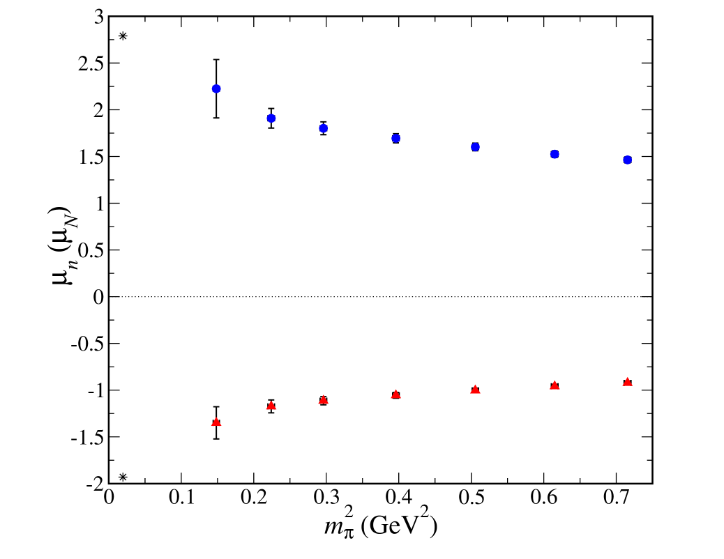
Figure 2: FLIC fermion simulation results for the magnetic moments of the proton (upper) and neutron (lower) in quenched QCD. The experimental values are given by asterisks

Figure 2 displays FLIC fermion simulation results for the magnetic moments of the proton and neutron in quenched QCD. The moments are obtained using the empirical fact that the $Q^{2}$ dependence of the electric and magnetic form factors of the proton over the range $0\to 0.23\ {\rm GeV}^{2}$ are nearly equivalent. At heavy quark masses we note that the magnetic moments of both nucleons display approximately linear behaviour when plotted as a function of $m_{\pi}^{2}$. Simulations at moderately heavier quark masses are expected to reveal a Dirac moment behavior $\propto~{}1/m_{q}\sim 1/m_{\pi}^{2}$. As one approaches the light quark mass regime, we find evidence of non-analytic behaviour in the nucleon magnetic moments as predicted by quenched $\chi$PT [1, 3]. In fact, if we were to flip the sign of the neutron magnetic moment, we would find that the proton and neutron have a very similar behaviour as a function of $m_{\pi}^{2}$ in the light quark mass regime as predicted by the leading non-analytic contributions of quenched $\chi$PT.

Figure 3: FLIC fermion simulation results for the charge radius of the proton in quenched QCD.

Figures 3 and 4 display results for the proton and neutron charge radii, respectively, obtained from a dipole form factor ansatz. For the proton some curvature is emerging as the chiral limit is approached. The FLIC fermion simulations reveal a small, negative value for the calculation of the quenched neutron charge radius at large and intermediate quark masses before the signal is lost at the lightest two quark masses. This result confirms the earlier result [15] that the two $d$ quarks have a larger charge radius than the $u$ quark within the neutron. This is also in agreement with quark model calculations [17].

Figure 4: FLIC fermion simulation results for the charge radius of the neutron in quenched QCD.

We also perform a calculation of the individual quark sector contributions to the magnetic moments. In Fig. 5 we show results for a calculation in quenched QCD of the ratio of singly to doubly represented quark magnetic contributions in the nucleon for quarks of unit charge. We see that our results deviate significantly from the simple quark model prediction of $-1/2$.

Figure 5: Ratio of singularly to doubly represented quark magnetic contributions in the nucleon for quarks of unit charge.

Figure 6 shows the results for a calculation of the octet $\Sigma$ baryons. We note the level ordering of the three $\Sigma$ baryons, with the positive and negative charge states both approaching the experimental values at light quark masses. We also see that our quenched lattice calculation of the magnetic moment of the neutral $\Sigma$ baryon predicts a value in the range $0.5-0.7\mu_{N}$, although we first need to take into account the appropriate chiral extrapolation and quenching effects [18] before an accurate prediction can be made. Our results reveal a significant amount of nonanalytic behaviour for the $\Sigma^{+}$, which is predicted by quenched $\chi$PT [3]. Q$\chi$PT also predicts a small amount of curvature for the $\Sigma^{0}$ and $\Sigma^{-}$ and we confirm this prediction [3].

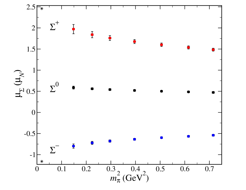
Figure 6: FLIC fermion simulation results for the magnetic moment of the octet $\Sigma$ baryons in quenched QCD.

We have also performed a calculation of the magnetic moment of the octet $\Xi$ baryons in quenched QCD and these results are shown in Fig. 7. Here we see an improved signal for the magnetic moment of the $\Xi$ compared to the other baryons at light quark masses due to the presence of two strange quarks. We note the splitting between the neutral and negative charged baryons is close to the experimentally observed value, even in the quenched approximation. Predictions from quenched chiral perturbation theory [3] suggest that there should be no nonanalytic behaviour for the $\Xi^{-}$ and a small amount of downward curvature for the $\Xi^{0}$. Our results confirm these predictions.

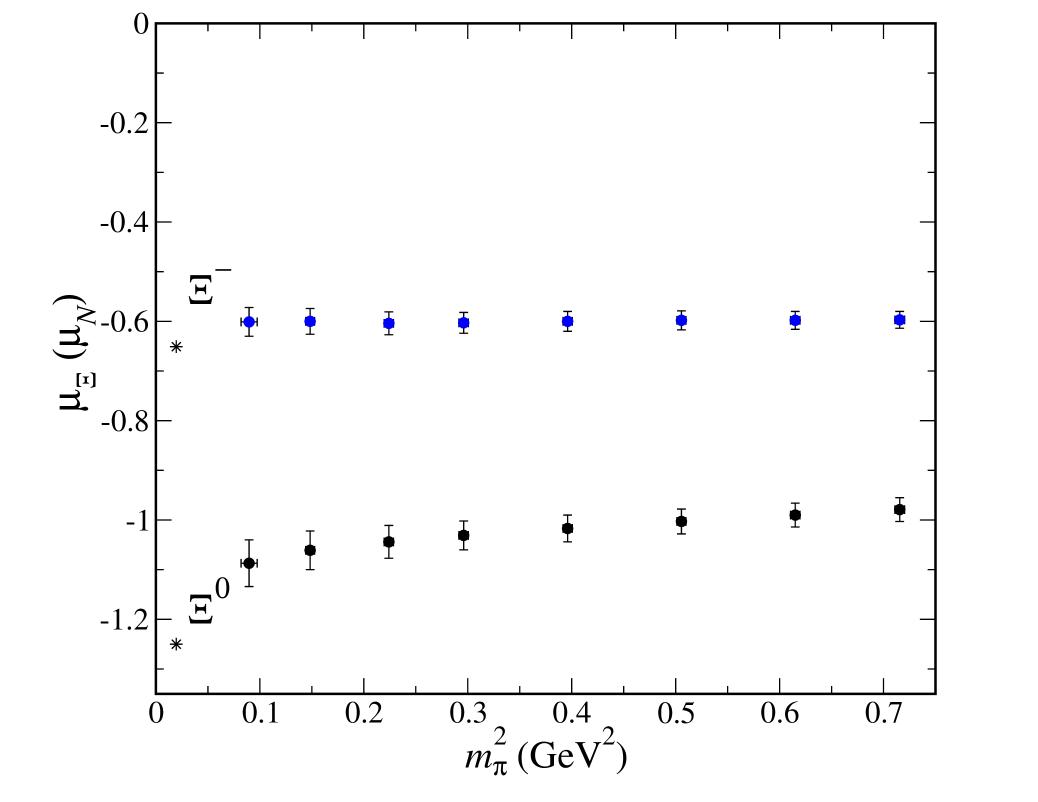
Figure 7: FLIC fermion simulation results for the magnetic moment of the octet $\Xi$ baryons in quenched QCD.

Figure 8 displays FLIC fermion simulation results for the magnetic moments of the proton and $\Delta^{+}$ resonance in quenched QCD. At large pion masses, the $\Delta$ moment is enhanced relative to the proton moment in accord with earlier lattice QCD results [15, 16] and model expectations. However as the chiral regime is approached the nonanalytic behavior of the quenched meson cloud is revealed, enhancing the proton and suppressing the $\Delta^{+}$ in accord with the expectations of quenched $\chi$PT [19, 20]. The quenched artifacts of the $\Delta$ provide an unmistakable signal for the onset of quenched chiral nonanalytic behavior.

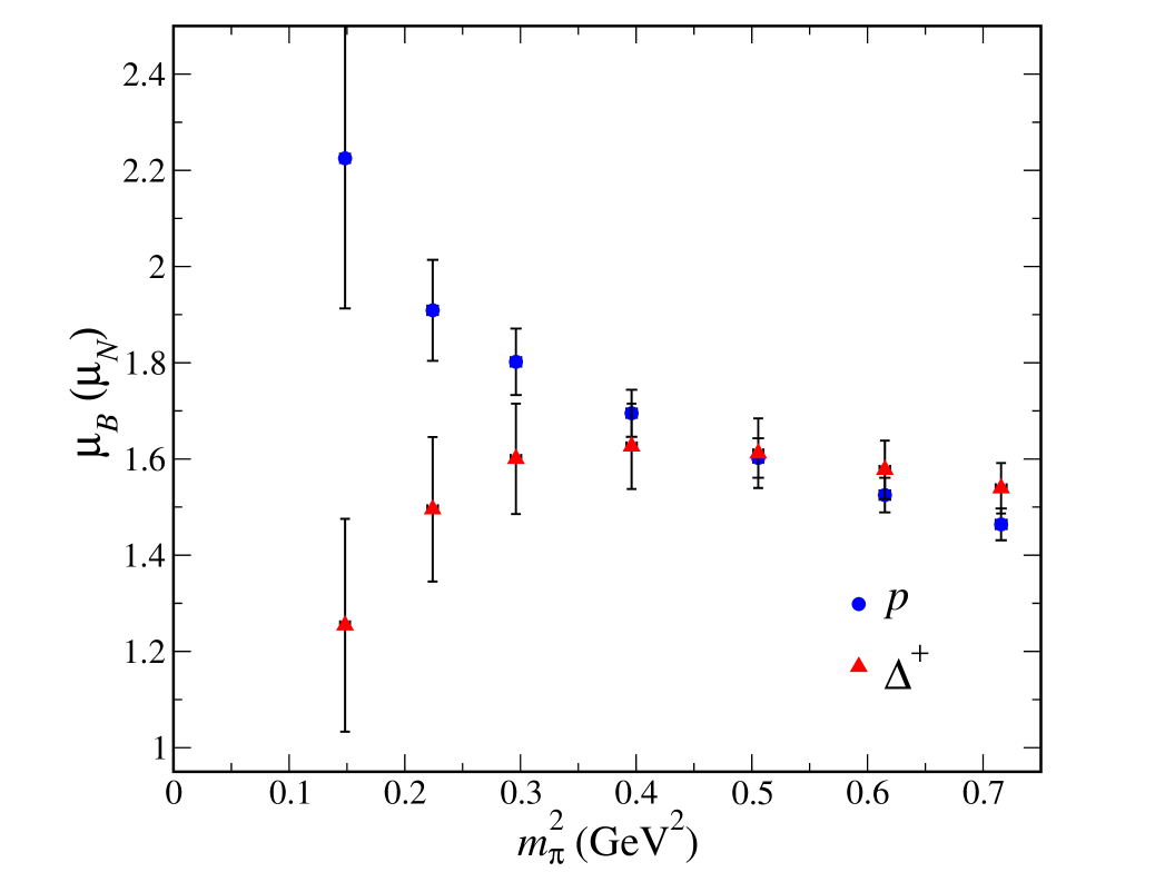
Figure 8: FLIC fermion simulation results for the magnetic moments of the proton ($\circ$) and $\Delta^{+}$ resonance ($\triangle$) in quenched QCD.

4 CONCLUSIONS

We have presented the first lattice QCD simulation results for the electromagnetic form factors of the nucleon, $\Sigma$, $\Xi$ and $\Delta$ baryons at quark masses light enough to reveal unmistakable quenched chiral nonanalytic behavior. The non-linear behaviour observed is in agreement with the predictions of quenched chiral perturbation theory [3, 20].

This work paves the way for a study of the individual quark sector contributions to baryon magnetic moments and, in particular, the strangeness content of the nucleon [18].

This work was supported by the Australian Research Council. We thank the Australian Partnership for Advanced Computing (APAC) for generous grants of supercomputer time which have enabled this project.

References

- [1] D. B. Leinweber, Nucl. Phys. Proc. Suppl. 109 (2002) 45 [hep-lat/0112021].
- [2] M. J. Savage, Nucl. Phys. A 700 (2002) 359 [nucl-th/0107038].
- [3] D. B. Leinweber, to appear in Phys. Rev. D, hep-lat/0211017.
- [4] J.M. Zanotti et al., Phys. Rev. D 60 (2002) 074507 [hep-lat/0110216]; Nucl.Phys.Proc.Suppl. 109 101 (2002) [hep-lat/0201004].
- [5] D. B. Leinweber, et al., nucl-th/0211014.
- [6] S. O. Bilson-Thompson, D. B. Leinweber and A. G. Williams, Annals Phys. 304 (2003) 1 [hep-lat/0203008].
- [7] M. Falcioni et al., Nucl. Phys. B251 (1985) 624; M. Albanese et al., Phys. Lett. B 192 (1987) 163.
- [8] J. Zanotti, et al., in preparation.
- [9] G. Martinelli, C. T. Sachrajda and A. Vladikas, Nucl. Phys. B 358 (1991) 212.
- [10] M. Luscher and P. Weisz, Commun. Math. Phys. 97, 59 (1985) [ibid. 98, 433 (1985)].
- [11] F.D. Bonnet et al., Phys. Rev. D 62 (2000) 094509 [hep-lat/0001018].
- [12] W. Kamleh, D. H. Adams, D. B. Leinweber and A. G. Williams, Phys. Rev. D 66, 014501 (2002) [hep-lat/0112041].
- [13] S. Gusken, Nucl. Phys. Proc. Suppl. 17, 361 (1990).
- [14] J. M. Zanotti, et al., Phys. Rev. D 68, 054506 (2003) [hep-lat/0304001].
- [15] D. B. Leinweber, R. M. Woloshyn and T. Draper, Phys. Rev. D 43 (1991) 1659.
- [16] D. B. Leinweber et al., Phys. Rev. D 46 (1992) 3067 [hep-lat/9208025].
- [17] R. D. Carlitz, S. D. Ellis and R. Savit, Phys. Lett. B 68, 443 (1977).
- [18] D. B. Leinweber, et al., these proceedings.
- [19] D. B. Leinweber, et al., nucl-th/0308083.
- [20] R. D. Young, D. B. Leinweber and A. W. Thomas, hep-lat/0309187; and hep-lat/0311038.