A numerical solution to the local cohomology problem in U(1) chiral gauge theories

Abstract

We consider a numerical method to solve the local cohomology problem related to the gauge anomaly cancellation in U(1) chiral gauge theories. In the cohomological analysis of the chiral anomaly, it is required to carry out the differentiation and the integration of the anomaly with respect to the continuous parameter for the interpolation of the admissible gauge fields. In our numerical approach, the differentiation is evaluated explicitly through the rational approximation of the overlap Dirac operator with Zolotarev optimization. The integration is performed with a Gaussian Quadrature formula, which turns out to show rather good convergence. The Poincaré lemma is reformulated for the finite lattice and is implemented numerically. We compute the current associated with the cohomologically trivial part of the chiral anomaly in two-dimensions and check its locality properties.

I Introduction

The construction of gauge-covariant and local lattice Dirac operators which satisfy the Ginsparg-Wilson relationGinsparg:1981bj ; Neuberger:1997fp ; Hasenfratz:1998ri ; Neuberger:1998wv ; Hasenfratz:1998jp ; Hernandez:1998et ; Luscher:1998pq ,

$$\gamma_{5}D+D\gamma_{5}=2aD\gamma_{5}D,$$ (1)

has made it possible to introduce Weyl fermions on the lattice and construct anomaly-free chiral gauge theories with exact gauge invarianceLuscher:1998kn ; Luscher:1998du ; Luscher:1999un ; Luscher:1999mt ; Luscher:2000hn footnote:overlap . One of the crucial steps in the gauge-invariant construction is to establish the exact cancellation of the gauge anomaly at a finite lattice spacing.

In the case of U(1) chiral gauge theoriesLuscher:1998du footnote:noncompact-u1 , the exact cancellation has been achieved through the cohomological classification of the chiral anomalyLuscher:1998kn ; Fujiwara:1999fi ; Fujiwara:1999fj footnote:nonabelian-anomaly . The anomaly is given in terms of lattice Dirac operatorLuscher:1998pq ; Kikukawa:1998pd ; Adams:1998eg ; Fujikawa:1998if ; Suzuki:1998yz ; Chiu:1998xf as

$$q(x)=\text{tr}\left\{\gamma_{5}(1-aD)(x,x)\right\}$$ (2)

and the local field $q(x)$ is a topological field in the sense that it satisfies

$$\sum_{x}\delta q(x)=0$$ (3)

under a local variation of the gauge field. It follows from this property that the anomaly is cohomologically trivial,

$$\sum_{\alpha}e_{\alpha}q^{\alpha}(x)=\partial_{\mu}^{\ast}k_{\mu}(x),\quad\quad q^{\alpha}(x)=\left.q(x)\right|_{U\rightarrow U^{e_{\alpha}}},$$ (4)

for an anomaly-free multiplet of Weyl fermions which satisfies the condition of the U(1) charges,

$$\sum_{\alpha}e_{\alpha}^{3}=0.$$ (5)

Here $k_{\mu}(x)$ is a gauge-invariant local current. This local current is in turn used in the gauge-invariant construction of the functional measure of the Weyl fermions.

If one thinks of the practical computation of observables in the lattice U(1) chiral gauge theories, it is required to compute the local current in Eq. (4) for every admissible gauge field. The purpose of this paper is to attempt a numerical computation of the local current. We will compute $k_{\mu}(x)$ in two-dimensions numerically and check its locality properties. We will also check how the exact cancellation of gauge anomaly works on the finite lattice.

This paper is organized as follows. In section II we formulate the vector-potential-representation of the link variables for the admissible U(1) gauge fields on the finite lattice. Using this representation, we introduce one-parameter families of the admissible fields for the interpolations. In section III we describe our numerical method to compute the bi-local current which is the first-differential of the chiral anomaly with respect to the vector potential. In section IV the Poincaré lemma is reformulated for a finite lattice so that we can carry out the cohomological analysis directly on the finite lattice. The result of the cohomological analysis in two-dimensions is summarized. In section V we describe our numerical result of the computation of the local current $k_{\mu}(x)$. Section VI is devoted to a summary and discussions.

II Admissible U(1) gauge fields          on a finite lattice

Our first step is to formulate the vector-potential-representation of the link variables associated with an admissible U(1) gauge field on a finite lattice. Such a representation has been formulated in the original cohomological analysis in Luscher:1998kn . However, it is constructed for the admissible gauge fields on the infinite lattice and the resulted vector-potentials are not bounded in general. This representation therefore does not seem to be useful for numerical implementations. But, as has been shown in our previous paperKadoh:2003ii , it is possible to formulate the bounded and periodic vector-potential representation for the admissible gauge fields on the finite lattice.

We set the lattice spacing $a$ to unity and consider U(1) gauge fields on a finite two- or four-dimensional lattice ($n=2,4$) of size $L$ with periodic boundary conditions. $L$ is assumed to be an even integer for simplicity. The gauge fields on such a lattice can be represented through periodic link fields on the infinite lattice,

$$U(x,\mu)\in{\rm U(1)},\quad x=(x_{1},x_{2},\cdots,x_{n})\in\mathbb{Z}^{n},$$ (6)

$$U(x+L\hat{\nu},\mu)=U(x,\mu)\ \ {\rm for\ all}\ \ \mu,\nu=1,\cdots,n.$$ (7)

The independent degrees of freedom are then the link variables at the points in the region

$$\Gamma_{n}=\left\{x\in\mathbb{Z}^{n}|-L/2\leq x_{\mu}<L/2\right\}.$$ (8)

As to gauge transformations

$$U(x,\mu)\rightarrow\Lambda(x)U(x,\mu)\Lambda(x+\hat{\mu})^{-1},$$ (9)

we consider only periodic functions $\Lambda(x)\in$ U(1) which preserves the periodicity of the link field.

We impose the admissibility condition on the U(1) gauge fields:

$$|F_{\mu\nu}(x)|<\epsilon\ \ {\rm for\ all}\ \ x,\mu,\nu,$$ (10)

where the field tensor $F_{\mu\nu}(x)$ is defined through

$$F_{\mu\nu}(x)=\frac{1}{i}{\rm ln}P_{\mu\nu}(x),\quad-\pi<F_{\mu\nu}(x)\leq\pi,$$ (11)

$$P_{\mu,\nu}(x)=U(x,\mu)U(x+\hat{\mu},\nu)U(x+\hat{\nu},\mu)^{-1}U(x,\nu)^{-1}.$$

We require this condition because it ensures that the overlap Dirac operatorNeuberger:1997fp ; Neuberger:1998wv , which we adopt in this work, is a smooth and local function of the gauge field for $|1-P_{\mu\nu}(x)|<1/30$ in four-dimensions and $|1-P_{\mu\nu}(x)|<1/5$ in two-dimensionsHernandez:1998et footnote:bound-neuberger . For $\epsilon<\pi/3$ the admissible U(1) gauge fields on the finite lattice can be classified uniquely by the magnetic fluxes $m_{\mu\nu}$ (integers independent of $x$) where

$$m_{\mu\nu}=\frac{1}{2\pi}\sum_{s,t=0}^{L-1}F_{\mu\nu}(x+s\hat{\mu}+t\hat{\nu}).$$ (13)

In this respect, the following field is periodic and can be shown to have constant field tensor equal to $2\pi m_{\mu\nu}/L^{2}$:

$$V_{[m]}(x,\mu)={\rm e}^{-\frac{2\pi i}{L^{2}}\left[L\delta_{\tilde{x}_{\mu},L-1}\sum_{\nu>\mu}m_{\mu\nu}\tilde{x}_{\nu}+\sum_{\nu<\mu}m_{\mu\nu}\tilde{x}_{\nu}\right]},$$ (14)

where the abbreviation $\tilde{x}_{\mu}=x_{\mu}$ mod $L$ has been used. Then any admissible U(1) gauge field in the topological sector with the magnetic flux $m_{\mu\nu}$ may be expressed as

$$U(x,\mu)=\tilde{U}(x,\mu)\,V_{[m]}(x,\mu).$$ (15)

We may regard $\tilde{U}(x,\mu)$ as the actual local and dynamical degrees of freedom in the given topological sector. This is because the magnetic flux $m_{\mu\nu}$ is invariant with respect to a local variation of the link field.

The following lemma shows that it is possible to establish the one-to-one correspondence between $\tilde{U}(x,\mu)$ and a periodic vector potential with the desired locality properties on the finite latticeKadoh:2003ii .

Lemma II   There exists a periodic vector potential $\tilde{A}_{\mu}(x)$ such that

$${\rm e}^{i\tilde{A}_{\mu}(x)}=\tilde{U}(x,\mu),$$ (16)

$$\partial_{\mu}\tilde{A}_{\nu}(x)-\partial_{\nu}\tilde{A}_{\mu}(x)=F_{\mu\nu}(x)-\frac{2\pi m_{\mu\nu}}{L^{2}},$$ (17)

$$\left\{\begin{array}[]{ll}|\tilde{A}_{\mu}(x)|\leq\pi(1+4\parallel x\parallel)&\parallel x\parallel\leq L/2\\ |\tilde{A}_{\mu}(x)|\leq\pi(1+2L+2(n-1)L^{2})&otherwise.\end{array}\right.$$ (20)

Moreover, if $\tilde{A}_{\mu}^{\prime}(x)$ is any other field with these properties, we have

$$\tilde{A}_{\mu}^{\prime}(x)=\tilde{A}_{\mu}(x)+\partial_{\mu}\omega(x),$$ (22)

where the gauge function $\omega(x)$ takes values that are integer multiples of $2\pi$. The explicit formula of $\tilde{A}_{\mu}(x)$ in two-dimensions is given in the appendix.

As emphasized in Luscher:1998kn , it is important to note that the locality properties of gauge invariant fields should be the same independently of whether they are considered to be functions of the link variables or the vector potential. Since the mapping

$$\tilde{A}_{\mu}(x)\rightarrow\tilde{U}(x,\mu)=\text{e}^{i\tilde{A}_{\mu}(x)}$$ (23)

is manifestly local, this is immediately clear if one starts with a field composed from the link variables. In the other direction, one may start from a gauge invariant local field $\phi(y)$ depending the vector potential. Then the key observation is that one is free to impose a complete axial gauge taking the point $y$ as the origin. Around $y$ the vector potential is locally constructed from the given link field and $\phi(y)$ thus maps to a local function of the link variables residing there.

The vector potential $\tilde{A}_{\mu}(x)$ represents an admissible field through ${\rm e}^{i\tilde{A}_{\mu}(x)}\times V_{[m]}(x,\mu)$ and the associated field tensor $F_{\mu\nu}(x)=\partial_{\mu}\tilde{A}_{\nu}(x)-\partial_{\nu}\tilde{A}_{\mu}(x)+\frac{2\pi m_{\mu\nu}}{L^{2}}$ is hence bounded by $\epsilon$. It is straightforward to check that this property is preserved if the potential is scaled by a factor $t$ in the range $0\leq t\leq 1$, i.e. we can contract the vector potential to zero without leaving the space of admissible fields. Then, in the cohomological analysis of the chiral anomaly, we may choose $V_{[m]}(x,\mu)$ as the reference gauge field in a given magnetic flux sector and may consider the interpolation between the arbitrary gauge field in the same sector and the reference field as follows:

$$U_{t}(x,\mu)={\rm e}^{it\tilde{A}_{\mu}(x)}\times V_{[m]}(x,\mu)\qquad t\in[0,1].$$ (24)

III Chiral anomaly and its topological properties

For our numerical application, we adopt the overlap Dirac operatorNeuberger:1997fp ; Neuberger:1998wv given by

$$D=\frac{1}{2}\left(1+\gamma_{5}\frac{H_{\rm w}}{\sqrt{H_{\rm w}^{2}}}\right),$$ (25)

where $H_{\rm w}$ is the Hermitian Wilson-Dirac operator,

$$H_{\rm w}=\gamma_{5}\left(\gamma_{\mu}\frac{1}{2}(\nabla_{\mu}-\nabla_{\mu}^{\dagger})+\frac{1}{2}\nabla_{\mu}\nabla_{\mu}^{\dagger}-m_{0}\right)$$ (26)

$(0<m_{0}<2)$. It is a smooth and local function of the admissible gauge field for $|1-P_{\mu\nu}(x)|<1/30$ in four-dimensions and for $|1-P_{\mu\nu}(x)|<1/5$ in two-dimensionsHernandez:1998et footnote:bound-neuberger . Then the chiral anomaly, Eq. (2), is given in terms of $H_{\rm w}$ as

$$q(x)=-\frac{1}{2}\text{tr}\left\{\frac{H_{\rm w}}{\sqrt{H_{\rm w}^{2}}}(x,x)\right\}.$$ (27)

As is clear from this expression, $q(x)$ is a topological field with respect to any local variation of the admissible gauge field,

$$\sum_{x}\delta q(x)=0.$$ (28)

This topological property of the chiral anomaly can be cast into properties of a certain gauge-invariant bi-local current. This bi-local current is defined through the differentiation and integration with respect to the continuous parameter $t$ for the interpolation as follows:

$$j_{\nu}(x,y)=\int_{0}^{1}dt\left(\frac{\partial q(x)}{\partial\tilde{A}_{\nu}(y)}\right)_{\tilde{A}\rightarrow t\tilde{A}}.$$ (29)

The original topological field can be expressed with the bi-local current as

$$q(x)=q_{[m]}(x)+\sum_{y\in\Gamma_{n}}j_{\nu}(x,y)\tilde{A}_{\nu}(y),$$ (30)

where $q_{[m]}(x)$ denotes the topological field for $V_{[m]}(x,\mu)$. Then the topological property and the gauge-invariance of $q(x)$ imply that $j_{\nu}(x,y)$ satisfies

$$\sum_{x\in\Gamma_{n}}j_{\nu}(x,y)=0,\qquad j_{\nu}(x,y)\overleftarrow{\partial_{\nu}^{\ast}}=0.$$ (31)

These conditions provide the initial conditions for the cohomological analysis.

For our purpose, it is required to compute the above bi-local current numerically keeping the conditions Eq. (31) within a given accuracy. Our strategy is the following. First of all, in order to obtain more explicit formula of the bi-local current, we introduce the parameter representation of the inverse square root of $H_{\rm w}^{2}$ as

$$\frac{H_{\rm w}}{\sqrt{H_{\rm w}^{2}}} = \int_{-\infty}^{\infty}\frac{dt}{\pi}\frac{H_{\rm w}}{t^{2}+H_{\rm w}^{2}}.$$ (32)

Then we can perform the differentiation of $q(x)$ with respect to the vector potential $\tilde{A}_{\mu}(x)$ explicitlyKikukawa:1998py as

$$\frac{\partial q(x)}{\partial\tilde{A}_{\nu}(y)} = -\frac{1}{2}{\rm tr}\left\{\int_{-\infty}^{\infty}\frac{dt}{\pi}\frac{1}{t^{2}+H_{\rm w}^{2}}\times\right.$$

$$\left.\left(t^{2}V_{\mu}(y)-H_{\rm w}V_{\mu}(y)H_{\rm w}\right)\frac{1}{t^{2}+H_{\rm w}^{2}}(x,x)\right\},$$

where

$$V_{\mu}(y) = -i\gamma_{5}\frac{1}{2}\left\{(1-\gamma_{\mu})\delta_{x,y}\delta_{x+\hat{\mu},z}U_{\mu}(x)\right.$$

$$\qquad\left.\,+(1+\gamma_{\mu})\delta_{y,z}\delta_{x,z+\hat{\mu}}U_{\mu}(z)^{-1}\right\}.$$

For the numerical evaluation of the differentiation, we then adopt the rational approximation of the overlap Dirac operatorNeuberger:1998my ; Edwards:1998yw with the Zolotarev optimizationChiu:2002eh ; vandenEshof:2002ms . Namely, $q(x)$ is approximated by the formula with the degree $N_{r}$:

$$q(x)\fallingdotseq-\frac{1}{2}{\rm tr}\left\{h_{\rm w}\sum_{k=1}^{N_{r}}\frac{b_{k}}{h_{\rm w}^{2}+c_{2k-1}}(x,x)\right\}.$$ (35)

$h_{\rm w}$ is defined by $H_{\rm w}/\lambda_{\rm min}$ where $\lambda_{\rm min}$ is the square root of the minimum of the eigenvalues of $H_{\rm w}^{2}$. The definitions of the coefficients $c_{k}$ and $b_{k}$ are given in the appendix. With this approximation, Eq. (III) can be approximated as follows:

$$\frac{\partial q(x)}{\partial\tilde{A}_{\nu}(y)} \fallingdotseq -\frac{1}{2}{\rm tr}\left\{\sum_{k=1}^{N_{r}}b_{k}\frac{1}{h_{\rm w}^{2}+c_{2k-1}}\times\right.$$

$$\left.\left(c_{2k-1}v_{\mu}(y)-h_{\rm w}v_{\mu}(y)h_{\rm w}\right)\frac{1}{h_{\rm w}^{2}+c_{2k-1}}(x,x)\right\},$$

where $v_{\mu}(y)=V_{\mu}(y)/\lambda_{\rm min}$. Finally, for the integration back with respect to the parameter for the interpolation in Eq. (29), we adopt the Gaussian Quadrature (Gauss-Legendre) formula with $N_{g}$ points:

$$j_{\nu}(x,y)\fallingdotseq\sum_{i=1}^{N_{g}}w_{i}\left(\frac{\partial q(x)}{\partial\tilde{A}_{\nu}(y)}\right)_{\tilde{A}\rightarrow t_{i}\tilde{A}},$$ (37)

where $\{(t_{i},w_{i})|i=1,\cdots,N_{g}\}$ is the set of the abscissas and weights of the degree $N_{g}$.

The formulae, Eqs. (III) and (37), are still complicated for the numerical computation. But, in two-dimensions, it is not demanding numerically for relatively small lattice sizes to diagonalize $H_{\rm w}$ and store all the eigenvectors. Namely, we can write

$$h_{\rm w}(x,y)=\sum_{\lambda}\psi_{\lambda}(x)\left(\frac{\lambda}{\lambda_{\rm min}}\right)\psi_{\lambda}^{\dagger}(y)$$ (38)

and then it is possible to evaluate Eqs. (III), (37) explicitly.

In this approximation, the gauge-invariance of the bi-local current and the second property of Eq. (31) can be preserved exactly. As to the first property of Eq. (31), we will see below that the choice $N_{r}=18$ and $N_{g}=20$ gives good convergences for the admissible gauge fields on the two-dimensional lattice of the size $L=8,10,12$ and the original topological field, $q(x)$, can be reproduced through Eq. (30) within the error less than $1\times 10^{-14}$.

IV Cohomological Analysis of chiral anomaly on a finite lattice

IV.1 The modified Poincaré lemma on a finite lattice

Our numerical cohomological analysis of the chiral anomaly will be performed directly on a finite lattice. For this purpose it is required to reformulate the Poincaré lemma on the latticeLuscher:1998kn for a finite lattice. For the detail of the proof of the lemmas, refer to our previous paperKadoh:2003ii .

In the following we will consider tensor fields $f_{\mu_{1}\cdots\mu_{k}}(x)$ on $\Gamma_{n}$ that are totally anti-symmetric in the indices $\mu_{1},\cdots,\mu_{k}$. Such tensor fields may be regarded as periodic tensor fields on the infinite lattice,

$$f_{\mu_{1}\cdots\mu_{k}}(x+L\hat{\nu})=f_{\mu_{1}\cdots\mu_{k}}(x)\ \ {\rm for\ all}\ \ \mu,\nu=1,\cdots,n.$$ (39)

The locality properties of such fields are assumed to be as follows: for a certain reference point $x_{0}\in\Gamma_{n}$ and $-L/2\leq(x_{\mu}-{x_{0}}_{\mu})<L/2$ (mod $L$),

$$|f_{\mu_{1}\cdots\mu_{k}}(x)| < C_{1}(1+\parallel x-x_{0}\parallel^{p_{1}})\,{\rm e}^{-\parallel x-x_{0}\parallel/\varrho},$$ (40)

$$\qquad\qquad\quad\left(\parallel x-x_{0}\parallel<L/2\right),$$

$$|f_{\mu_{1}\cdots\mu_{k}}(x)| < C_{2}L^{p_{2}}\,{\rm e}^{-L/2\varrho},$$ (41)

$$\qquad\qquad\quad\left(\parallel x-x_{0}\parallel\geq L/2\right).$$

$\varrho$ is a localization range of the tensor field. $C_{i}$ and $p_{i}\geq 0$ are certain constants that do not depend on $L$. $\parallel x-x_{0}\parallel$ is the taxi driver distance from $x_{0}$ to $x$. This locality properties hold true for the differentials of the chiral anomaly given in terms of overlap Dirac operatorNeuberger:1997fp ; Neuberger:1998wv with respect to the admissible gauge fieldsHernandez:1998et footnote:lemma-for-superlocal-field .

The differential forms on the finite lattice are introduced as in the continuum, following Luscher:1998kn . If we adopt the Einstein summation convention for tensor indices, the general $k$-form on $\Gamma_{n}$ is then given by

$$f(x)=\frac{1}{k!}f_{\mu_{1}\cdots\mu_{k}}(x)dx_{\mu_{1}}\cdots dx_{\mu_{k}}.$$ (42)

The linear space of all these forms is denoted by $\Omega_{k}$. An exterior difference operator ${\rm d}:\Omega_{k}\rightarrow\Omega_{k+1}$ may now be defined through

$$df(x)=\frac{1}{k!}\partial_{\mu}f_{\mu_{1},\cdots,\mu_{k}}(x)dx_{\mu}dx_{\mu_{1}}\cdots dx_{\mu_{k}},$$ (43)

where $\partial_{\mu}$ denotes the forward nearest-neighbor difference operator. The associated divergence operator $d^{\ast}:\Omega_{k}\rightarrow\Omega_{k-1}$ is defined in the obvious way by setting $d^{\ast}f=0$ if $f$ is a 0-form and

$$d^{\ast}f(x)=\frac{1}{(k-1)!}\partial_{\mu}^{\ast}f_{\mu\mu_{2}\cdots\mu_{k}}(x)dx_{\mu_{2}}\cdots dx_{\mu_{k}}$$ (44)

in all other cases, where $\partial_{\mu}^{\ast}$ is the backward nearest-neighbor difference operator.

By definition, the divergence operator satisfies that ${d^{\ast}}^{2}=0$ and therefore the difference equation $d^{\ast}f=0$ is solved by all forms $f=d^{\ast}g$. It has been shown that in the infinite lattice these are in fact all solutions, an exception being the $0$-forms where one has a one-dimensional space of further solutionsLuscher:1998kn . This result is the lattice counter part of the Poincaré lemma known in the continuum theory. On the finite periodic lattice the lemma does not hold true any more, because the lattice is a n-dimensional torus and its cohomology group is now non-trivial. However, the lemma can be reformulated so that it holds true up to exponentially small correction terms of order ${\cal O}({\rm e}^{-L/2\varrho})$ and for the form satisfying $\sum_{x\in\Gamma_{n}}f(x)=0$, it holds exactly even on the finite lattice.footnote:lemma-for-superlocal-field The latter result is the lattice counter part of the corollary of de Rham theorem known in the continuum theory. The precise statements are the following.footnote:lemma-in-d

Lemma IV.a   (Modified Poincaré lemma)

Let $f$ be a $k$-form which satisfies

$$d^{\ast}f=0\ \ \ {\rm and}\ \ \ \sum_{x\in\Gamma_{n}}f(x)=0\ \ {\rm if}\ \ k=0.$$ (45)

Then there exist a form $g\in\Omega_{k+1}$ and a form $\Delta f\in\Omega_{k}$ such that

$$f=d^{\ast}g+\Delta f,\qquad|\Delta f_{\mu_{1}\cdots\mu_{k}}(x)|<cL^{\sigma}{\rm e}^{-L/2\varrho}.$$ (46)

Lemma IV.b   (Corollary of de Rham theorem)

Let $f$ be a $k$-form which satisfies

$$d^{\ast}f=0\ \ {\rm and}\ \ \sum_{x\in\Gamma_{n}}f(x)=0.$$ (47)

Then there exist a form $g\in\Omega_{k+1}$ such that

$$f=d^{\ast}g.$$ (48)

The explicit formula of $g(x)$ in two-dimensions ($n=2$) is given in the appendix.

IV.2 A solution to the local cohomology problem
on the two-dimensional finite lattice

In two dimensions, the cohomological analysis results in the following formula for $q(x)$:

$$q(x)={\cal A}(x)+\partial_{\mu}^{\ast}h_{\mu}(x)+\Delta q(x),$$ (49)

where

$${\cal A}(x)=q_{[m]}(x)+\phi_{\mu\nu}(x)\,\tilde{F}_{\mu\nu}(x),\quad\partial_{\mu}^{\ast}\phi_{\mu\nu}(x)=0.$$ (50)

$\phi_{\mu\nu}(x)$ is obtained through the applications of the modified Poincaré lemma and the corollary of the de Rham theorem:

$$j_{\nu}(x,y) \xrightarrow{\text{IV.a}} \theta_{\nu\mu}(x,y)\overleftarrow{\partial_{\mu}^{\ast}}+\Delta j_{\nu}(x,y),$$ (51)

$$\sum_{z\in\Gamma_{2}}\Delta j_{\nu}(z,x) \xrightarrow{\text{IV.b}} -2\,\Delta\Phi_{\nu\mu}(x)\overleftarrow{\partial_{\mu}^{\ast}}$$ (52)

and

$$\phi_{\mu\nu}(x) \equiv \frac{1}{2}\sum_{z\in\Gamma_{2}}\theta_{\mu\nu}(z,x)-\Delta\Phi_{\mu\nu}(x).$$ (53)

In two-dimensions, $\phi_{\mu\nu}(x)$ is a constant and assumes the form $\phi_{\mu\nu}(x)=\gamma_{[m,w]}\epsilon_{\mu\nu}$. $h_{\mu}(x)$ is obtained through the application of the modified Poincaré lemma:

$$\theta_{\mu\nu}(x,y)-\delta_{x,y}\sum_{z\in\Gamma_{2}}\theta_{\mu\nu}(z,y) \xrightarrow{\text{IV.a}} \partial_{\lambda}^{\ast}\tau_{\lambda\mu\nu}(x,y)$$

and

$$h_{\mu}(x) \equiv \frac{1}{2}\sum_{y\in\Gamma_{2}}\tau_{\mu\nu\rho}(x,y)\tilde{F}_{\nu\rho}(y).$$ (55)

$\Delta q(x)$ is defined by

$$\Delta q(x) \equiv \Delta\Phi_{\mu\nu}(x)\tilde{F}_{\mu\nu}(x)+\sum_{y\in\Gamma_{2}}\Delta j_{\nu}(x,y)\tilde{A}_{\nu}(y).$$

For the anomaly-free multiplet satisfying the condition $\sum_{\alpha}e_{\alpha}^{2}=0$, the anomaly part ${\cal A}(x)=q_{[m]}(x)+\gamma_{[m]}\epsilon_{\mu\nu}\tilde{F}_{\mu\nu}(x)$ cancels up to an exponentially small term,

$$\sum_{\alpha}e_{\alpha}{\cal A}^{\alpha}(x)=\Delta{\cal A}(x),$$ (57)

where ${\cal A}^{\alpha}(x)=\left.{\cal A}(x)\right|_{U\rightarrow U^{e_{\alpha}}}$. Since $\sum_{x\in\Gamma_{2}}\Delta{\cal A}(x)=0$, we may apply the modified Poincaré lemma IV.a to obtain

$$\Delta{\cal A}(x) \xrightarrow{\text{IV.a}} \partial_{\mu}^{\ast}\Delta k_{\mu}(x).$$ (58)

On the other hand, since $\sum_{x\in\Gamma_{2}}\Delta q(x)=0$, we may also apply the lemma IV.b as follows:

$$\Delta q(x) \xrightarrow{\text{IV.b}} \partial_{\mu}^{\ast}\Delta h_{\mu}(x).$$ (59)

Then we can see that $q(x)$ is cohomologically trivial,

$$\sum_{\alpha}e_{\alpha}q^{\alpha}(x)=\partial_{\mu}^{\ast}k_{\mu}(x),$$ (60)

where $k_{\mu}(x)$ is given explicitly as

$$k_{\mu}(x)\equiv\sum_{\alpha}e_{\alpha}\{h_{\mu}(x)+\Delta h_{\mu}(x)\}^{\alpha}+\Delta k_{\mu}(x).$$ (61)

Therefore, once the bi-local current $j_{\mu}(x,y)$ is computed, the current $k_{\mu}(x)$ can be obtained by the sequence of the applications of the lemmas IV.a,b. The numerical implementation of this step is straightforward using the explicit solutions, $g(x)$, of the lemmas given in the appendix.

V Numerical results

We now describe our result of numerical computations of the local current $k_{\mu}(x)$. We consider the lattice sizes $L=8,10,12$. Admissible gauge fields are generated by Monte Carlo simulation using the action

$$S=\frac{1}{4e^{2}}\sum_{x,\mu\nu}\frac{F_{\mu\nu}(x)^{2}}{1-F_{\mu\nu}(x)^{2}/\epsilon^{2}}=\beta\sum_{\square}\frac{F_{\square}^{2}}{1-F_{\square}^{2}/\epsilon^{2}}.$$ (62)

As reported in Fukaya:2003ph , the topological charge is preserved during the Monte Carlo updates with this type of action, even when $\epsilon$ is set to $\pi$. We adopt this option and check the locality of the topological field numerically for several values of $\beta$. We consider the topological sectors with $m_{12}=0,1$ and the initial configuration is chosen as $V_{[m]}(x,\mu)$ with a given $m_{12}$.

For each admissible gauge field, we compute the vector potential $\tilde{A}_{\mu}(x)$ formulated in section II. We also compute the abscissas and weights $\{(t_{i},w_{i})|\ i=1,\cdots,N_{g}\}$ for Gaussian Quadrature formula with the degree $N_{g}$. By this, the discrete interpolation of the given admissible gauge field is fixed:

$$\left\{U^{(i)}(x,\mu)={\rm e}^{it_{i}\tilde{A}_{\mu}(x)}\times V_{[m]}(x,\mu)\ \big{|}\ \ i=1,\cdots,N_{g}\right\}.$$ (63)

In table 1, the abscissas and weights for the degree $N_{g}=20$ are shown.

Table 1: The abscissas and weights for the Gauss-Legendre formula are shown for $N_{g}=20$. $t\in[0,1]$.

	$t_{i}$	$w_{i}$
1	3.435700407452558E-003	8.807003569576136E-003
2	1.801403636104310E-002	2.030071490019346E-002
3	4.388278587433703E-002	3.133602416705449E-002
4	8.044151408889061E-002	4.163837078835234E-002
5	0.126834046769925	5.096505990862024E-002
6	0.181973159636742	5.909726598075923E-002
7	0.244566499024586	6.584431922458825E-002
8	0.313146955642290	7.104805465919108E-002
9	0.386107074429177	7.458649323630189E-002
10	0.461736739433251	7.637669356536294E-002
11	0.538263260566749	7.637669356536294E-002
12	0.613892925570823	7.458649323630189E-002
13	0.686853044357710	7.104805465919108E-002
14	0.755433500975414	6.584431922458825E-002
15	0.818026840363258	5.909726598075923E-002
16	0.873165953230075	5.096505990862024E-002
17	0.919558485911109	4.163837078835234E-002
18	0.956117214125663	3.133602416705449E-002
19	0.981985963638957	2.030071490019346E-002
20	0.996564299592547	8.807003569576136E-003

For each $U^{(i)}(x,\mu)$, all eigenvalues and eigenvectors of $H_{\rm w}$ are computed numerically using the Householder method. We choose $m_{0}=0.9$ in $H_{\rm w}$. Then we compute the bi-local current $j_{\nu}(x,y)$ through Eqs. (III) and (37).

We can check the convergence of the above procedure through Eq. (30) by computing the deviation

$$\chi={\rm max}_{x\in\Gamma_{2}}\left|\delta(x)\right|,$$ (64)

where

$$\delta(x)=q(x)-q_{[m]}(x)-\sum_{y\in\Gamma_{2}}j_{\nu}(x,y)\tilde{A}_{\nu}(y).$$ (65)

Here the original topological fields $q(x)$ and $q_{[m]}(x)$ are constructed by computing all eigenvalues and eigenvectors of $H_{\rm w}$ for the given admissible gauge field $U(x,\mu)$ and for the reference gauge field $V_{[m]}(x,\mu)$, respectively. In this computation, we found that the topological fields have typically the values of order $O(10^{-2})-O(10^{-3})$. The integer topological charge $Q=\sum_{x\in\Gamma_{2}}q(x)=m_{12}$ is reproduced within the error of order $O(10^{-12})-O(10^{-13})$. In table 2, we show the dependence of $\chi$ on the degree $N_{g}$ with $N_{r}=18$, $L=8$ and $\beta=3.0$ fixed.

Table 2: The convergence of the bi-local current is shown for various values of $N_{g}$ with $N_{r}=18,L=8,\beta=3.0$ fixed.

$N_{g}$	$\chi$
4	$O(10^{-8})$
6	$O(10^{-12})$
8	$O(10^{-14})$
10	$O(10^{-15})$
12	$O(10^{-15})$
16	$O(10^{-15})$

For the larger lattice sizes $L=10,12$, we found that $\chi$ is less than $1\times 10^{-14}$ with the choice of $N_{g}=20$ and $N_{r}=18$.

Once the bi-local current $j_{\mu}(x,y)$ is computed, the cohomological analysis of the chiral anomaly can be performed numerically by the sequence of the applications of the lemmas. The result can be expressed as (cf. Eq. (49) )

$$q(x)={\cal A}(x)+\partial_{\mu}^{\ast}h_{\mu}(x)+\Delta q(x),$$ (66)

where

$${\cal A}(x)=q_{[m]}(x)+\gamma_{[m,w]}\epsilon_{\mu\nu}\,\tilde{F}_{\mu\nu}(x).$$ (67)

In order to check the locality properties of the fields, $q(x)$, ${\cal A}(x)$, $h_{\mu}(x)$ and $\Delta q(x)$, we apply a small local variation to the given admissible gauge field as $U(x,\mu)\rightarrow{\rm e}^{i\eta_{\mu}(x)}U(x,\mu)$ where

$$\eta_{\mu}(x)=0.05\times 2\pi\,\delta_{x,x_{0}}\delta_{\mu,1}$$ (68)

and compute the variations of the fields. For each variation of the fields, $\delta_{\eta}f(x)$, we define

$$\delta_{\eta}f(r)=\text{max}\left\{|\delta_{\eta}f(x)|\big{|}\,r=\parallel x-x_{0}\parallel\right\}$$ (69)

and see the locality properties of the fields by plotting $\delta_{\eta}f(r)$ against $r=\parallel x-x_{0}\parallel$. For the anomaly part ${\cal A}(x)$, the variation of $\gamma_{[m,w]}$ is considered.

The results are shown in figures 1, 2 and 3 for $\beta=3.0$. In figure 1, the variation of the topological field $q(x)$ is shown. The locality of the topological field $q(x)$ is clearly seen. We can read the locality range as $\varrho\simeq 0.5$. The maximum value of the field $\Delta q(x)$ is also shown in the same figure. We can confirm that

$$|\Delta q(x)|\simeq O(10^{-5})\simeq O({\rm e}^{-L/2\varrho})\quad(L=12).$$ (70)

In figure 2, the variations of the current $h_{\mu}(x)$ are shown. It shows clearly that the current $h_{\mu}(x)$ has the same locality property as the topological field $q(x)$ has and thus is local. In figure 3, the variations of the anomaly coefficient $\gamma_{[m,w]}$ and the field $\Delta q(x)$ are shown. We can confirm that the gauge field dependence of $\gamma_{[m,w]}$ is indeed small and the same order of magnitude as the size of $\Delta q(x)$ and its variation.

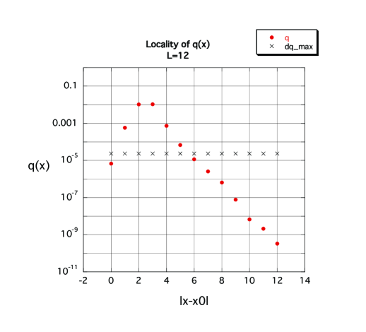
Figure 1: The variation of the topological field $\delta_{\eta}q(r)$(filled circle) is plotted against $r=\parallel x-x_{0}\parallel$. The maximum value of $|\Delta q(x)|$ (cross) is also shown. The lattice size is $L=12$. The gauge field is generated at $\beta=3.0$ with the vanishing magnetic flux $m_{12}=0$.

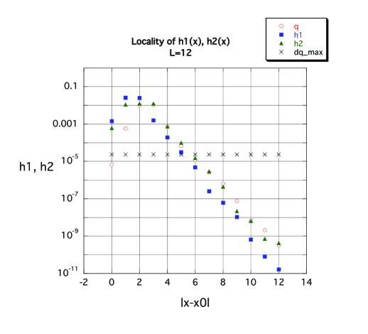
Figure 2: The variations $\delta_{\eta}h_{\mu}(r)$ are plotted against $r=\parallel x-x_{0}\parallel$ (filled square and triangle). For a guide, the variation $\delta_{\eta}q(r)$ (open circle) and the maximum value of $|\Delta q(x)|$(cross) are also shown.

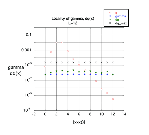
Figure 3: The variations $\delta_{\eta}\gamma_{[m,w]}$(filled diamond) and $\delta_{\eta}\Delta q(r)$ (filled triangle) are plotted against $r=\parallel x-x_{0}\parallel$ . For a guide, the variation $\delta_{\eta}q(r)$ (open circle) and the maximum value of $|\Delta q(x)|$(cross) are also shown.

The locality properties of the fields $q(x)$, ${\cal A}(x)$, $h_{\mu}(x)$ and $\Delta q(x)$ are confirmed also for topologically non-trivial gauge fields. See figure 4.

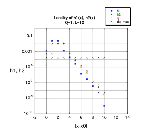
Figure 4: The variations $\delta_{\eta}h_{\mu}(r)$ are plotted against $r=\parallel x-x_{0}\parallel$ (filled square and triangle). For a guide, the variation $\delta_{\eta}q(r)$ (open circle) and the maximum value of $|\Delta q(x)|$(cross) are also shown. The lattice size is $L=10$. The gauge field is generated at $\beta=3.0$ with the magnetic flux $m_{12}=1$.

We next examine the cancellation of the gauge anomaly. We consider the so-called 11112 model which consists of four Left-handed Weyl fermions with unit charge and one Right-handed Weyl fermion with charge two. The gauge anomaly cancellation condition in two-dimensions is satisfied as follows:

$$\sum_{i=1}^{4}e^{2}-(2e)^{2}=0.$$ (71)

In figure 5, we plot the anomaly parts of the Left-handed fermions $4\times{\cal A}^{1}(x)$ and of the Right-handed fermion ${\cal A}^{2}(x)$, where ${\cal A}^{\alpha}(x)=\left.{\cal A}(x)\right|_{U\rightarrow U^{e_{\alpha}}}$, and the total anomaly part $\sum_{\alpha}{\cal A}^{\alpha}(x)=4\times{\cal A}^{1}(x)-{\cal A}^{2}(x)$ for $\beta=3.0$ and $m_{12}=0$. The result is impressive. The size of the total anomaly part is reduced to the order $O({\rm e}^{-L/2\varrho})$ after the cancellation and we can confirm that

$$\Delta{\cal A}(x)\simeq O({\rm e}^{-L/2\varrho})\simeq O(10^{-4})\quad(L=10).$$ (72)

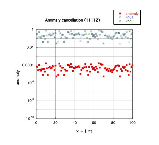
Figure 5: The anomaly parts of the Left-handed fermions $4\times{\cal A}^{1}(x)$ (open circle) and of the Right-handed fermion ${\cal A}^{2}(x)$ (cross) are plotted against the fused coordinate $x+L\times t$. The total anomaly part $4\times{\cal A}^{1}(x)-{\cal A}^{2}(x)$ (filled rectangle) is also plotted. The lattice size is $L=10$. The gauge field is generated at $\beta=3.0$ with the vanishing magnetic flux $m_{12}=0$.

This result is also confirmed in figure 6. In this figure, the total topological field $\sum_{\alpha}q^{\alpha}(x)$, the total anomaly part $\sum_{\alpha}{\cal A}^{\alpha}(x)$ and the total finite volume correction $\sum_{\alpha}\Delta q^{\alpha}(x)$ are plotted. We see clearly that the size of $\Delta{\cal A}(x)$ is the same order of magnitude as the size of $\Delta q(x)$. The similar cancellation is also observed for topologically non-trivial gauge fields with $m_{12}=1$.

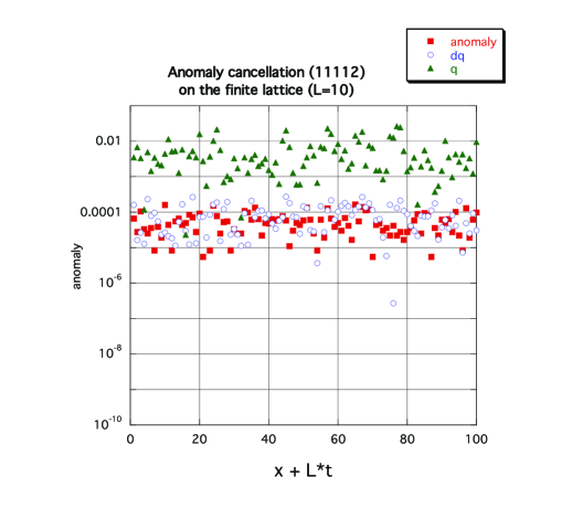
Figure 6: The total topological field $\sum_{\alpha}q^{\alpha}(x)$ (filled triangle), the total anomaly part $\sum_{\alpha}{\cal A}^{\alpha}(x)$ (filled rectangle) and the total finite volume correction $\sum_{\alpha}\Delta q^{\alpha}(x)$ (open circle) are plotted against the fused coordinate $x+L\times t$.

Now the current $k_{\mu}(x)$ can be computed from Eqs. (58), (59) and (61). The current so obtained is thus local. This local current can reproduce the original topological charge $q(x)$ within the deviation of order $O(10^{-15})$. The gauge invariance of the current is also maintained within the error.

VI Discussion

We have demonstrated that the cohomological analysis of the chiral anomaly associated with the overlap fermions can be performed numerically in two-dimensional lattice with a finite volume. The resulted current $k_{\mu}(x)$ is gauge invariant and local.

Four-dimensional case is numerically demanding. The evaluation of the differential of the topological fields should be performed without diagonalizing $H_{\rm w}$. For other parts, our procedure would work also in this case.

Our next step would be the numerical construction of the Weyl fermions measures and observables in the anomaly-free U(1) chiral gauge theories in two-dimensions, keeping the gauge invariance. Work in this direction is in progress.

Appendix A

In this appendix, we give the explicit formulae for the vector-potential representation of the link variables of the admissible U(1) gauge field discussed in the section II. We first define

$$\tilde{a}_{\mu}(x)\equiv\frac{1}{i}\ln\{U(x,\mu)V_{[m]}(x,\mu)^{-1}\}$$ (73)

and

$$2\pi\tilde{n}_{\mu\nu}(x)\equiv F_{\mu\nu}(x)-\frac{2\pi m_{\mu\nu}}{L^{2}}-\{\partial_{\mu}\tilde{a}_{\nu}(x)-\partial_{\nu}\tilde{a}_{\mu}(x)\}.$$ (74)

We also introduce a summation convention as

$$\sum_{t_{i}=0}^{x_{i}-1}{}^{\prime}f(x)=\left\{\begin{array}[]{ll}\sum_{t_{i}=0}^{x_{i}-1}f(x)&(x_{i}\geq 1)\\ 0&(x_{i}=0)\\ \sum_{t_{i}=x_{i}}^{-1}(-1)f(x)&(x_{i}\leq-1)\end{array}\right..$$ (75)

Then, in four-dimensions, the vector-potential is defined by

$$\tilde{A}_{4}(x) = \tilde{a}_{4}(x)+2\pi\left\{\sum_{t_{1}=0}^{x_{1}-1}{}^{\prime}\tilde{n}_{14}(x)+\sum_{t_{2}=0}^{x_{2}-1}{}^{\prime}2\pi\tilde{n}_{24}(x)|_{x_{1}=0}\right.$$

$$\left.+\sum_{t_{3}=0}^{x_{3}-1}{}^{\prime}\tilde{n}_{34}(x)|_{x_{1}=x_{2}=0}\right\},$$

$$\tilde{A}_{3}(x) = \tilde{a}_{3}(x)+2\pi\left\{\sum_{t_{1}=0}^{x_{1}-1}{}^{\prime}\tilde{n}_{13}(x)+\sum_{t_{2}=0}^{x_{2}-1}{}^{\prime}\tilde{n}_{23}(x)|_{x_{1}=0}\right.$$

$$\left.-\delta_{x_{3},L/2-1}\sum_{t_{4}=0}^{x_{4}-1}{}^{\prime}\sum_{t_{3}=-L/2}^{L/2-1}\tilde{n}_{34}(x)|_{x_{1}=x_{2}=0}\right\},$$

$$\tilde{A}_{2}(x) = \tilde{a}_{2}(x)+2\pi\left\{\sum_{t_{1}=0}^{x_{1}-1}{}^{\prime}\tilde{n}_{12}(x)\right.$$

$$-\delta_{x_{2},L/2-1}\sum_{t_{3}=0}^{x_{3}-1}{}^{\prime}\sum_{t_{2}=-L/2}^{L/2-1}\tilde{n}_{23}(x)|_{x_{1}=0,x_{4}=0}$$

$$\left.-\delta_{x_{2},L/2-1}\sum_{t_{4}=0}^{x_{4}-1}{}^{\prime}\sum_{t_{2}=-L/2}^{L/2-1}\tilde{n}_{24}(x)|_{x_{1}=0}\right\},$$

$$\tilde{A}_{1}(x) = \tilde{a}_{1}(x)+2\pi\left\{\phantom{-\delta_{x_{1},L/2-1}\sum_{t_{2}=0}^{x_{2}-1}{}^{\prime}\sum_{t_{1}=-L/2}^{L/2-1}\tilde{n}_{12}(x)|_{x_{3}=x_{4}=0}}\right.$$

$$-\delta_{x_{1},L/2-1}\sum_{t_{2}=0}^{x_{2}-1}{}^{\prime}\sum_{t_{1}=-L/2}^{L/2-1}\tilde{n}_{12}(x)|_{x_{3}=x_{4}=0}$$

$$-\delta_{x_{1},L/2-1}\sum_{t_{3}=0}^{x_{3}-1}{}^{\prime}\sum_{t_{1}=-L/2}^{L/2-1}\tilde{n}_{13}(x)|_{x_{4}=0}$$

$$\left.-\delta_{x_{1},L/2-1}\sum_{t_{4}=0}^{x_{4}-1}{}^{\prime}\sum_{t_{1}=-L/2}^{L/2-1}\tilde{n}_{14}(x)\right\}.$$

In two-dimensions, the vector potential is defined by

$$\tilde{A}_{2}(x) = \tilde{a}_{2}(x)+2\pi\sum_{t_{1}=0}^{x_{1}-1}{}^{\prime}\tilde{n}_{12}(x),$$

$$\tilde{A}_{1}(x) = \tilde{a}_{1}(x)$$

$$-\delta_{x_{1},L/2-1}\sum_{t_{2}=0}^{x_{2}-1}{}^{\prime}\sum_{t_{1}=-L/2}^{L/2-1}2\pi\tilde{n}_{12}(x).$$

Appendix B Rational approximation of the Overlap Dirac operator

In this appendix, we give the formula of the rational approximation of the overlap Dirac operator with the Zolotarev optimization. The inverse square root of $H_{\rm w}^{2}$ times $H_{\rm w}$ is approximated by

$$\frac{H_{\rm w}}{\sqrt{H_{\rm w}^{2}}}=h_{\rm w}\sum_{k=1}^{n}\frac{b_{k}}{h_{\rm w}^{2}+c_{2k-1}}.$$ (77)

$h_{\rm w}$ is defined by $H_{\rm w}/\lambda_{\rm min}$ where $\lambda_{\rm min}$ is the square root of the minimum of the eigenvalues of $H_{\rm w}^{2}$, and the coefficients $c_{k}$ and $b_{k}$ are given as follows:

$$c_{k} = \frac{{\rm sn}^{2}\left(\frac{kK^{\prime}}{2n};\kappa^{\prime}\right)}{1-{\rm sn}^{2}\left(\frac{kK^{\prime}}{2n};\kappa^{\prime}\right)},$$ (78)

$$\lambda = \prod_{k=1}^{2n}\frac{\Theta^{2}\left(\frac{2kK^{\prime}}{2n};\kappa^{\prime}\right)}{\Theta^{2}\left(\frac{(2k-1)K^{\prime}}{2n};\kappa^{\prime}\right)},$$ (79)

$$d_{0} = \frac{2\lambda}{\lambda+1}\prod_{k=1}^{n}\frac{1+c_{2k-1}}{1+c_{2k}},$$ (80)

$$b_{k} = d_{0}\frac{\prod_{i=1}^{n-1}(c_{2i}-c_{2k-1})}{\prod_{i=1,i\not=k}^{n}(c_{2i-1}-c_{2k-1})}.$$ (81)

$K^{\prime}$ is the complete elliptic integral of the first kind with modulus $\kappa^{\prime}=\sqrt{1-(\lambda_{\rm min}/\lambda_{\rm max})^{2}}$.

Appendix C Solutions of the Modified Poincaré lemma and the corollary of de Rham theorem in two-dimensions

In this appendix, we give the explicit solutions of the Poincaré lemma in two-dimensions (n=2).

IV.a(0-form) and IV.b(0-form):

$$g_{1}(x_{1},x_{2})=\delta_{x_{2},x^{0}_{2}}\sum_{y_{1}=x^{0}_{1}-L/2}^{x_{1}}\bar{f}(y_{1}),$$

$$g_{2}(x_{1},x_{2})=\sum_{y_{2}=x^{0}_{2}-L/2}^{x_{2}}\left\{f(x_{1},y_{2})-\delta_{y_{2},x^{0}_{2}}\bar{f}(x_{1})\right\},$$

where $\bar{f}(x_{1})=\sum_{y_{2}=-L/2}^{L/2-1}f(x_{1},y_{2})$.

IV.a(1-form):

$$g_{12}(x_{1},x_{2})=-\sum_{y_{2}=x^{0}_{2}-L/2}^{x_{2}}\left\{f_{1}(x_{1},y_{2})-\delta_{y_{2},x^{0}_{2}}\bar{f}_{1}(x_{1})\right\},$$

$$\Delta f_{1}(x_{1},x_{2})=\delta_{x_{2},x^{0}_{2}}\bar{f}_{1}(x_{1}),$$

$$\Delta f_{2}(x_{1},x_{2})=f_{2}(x_{1},x_{2})|_{x_{2}=x^{0}_{2}-L/2-1},$$ (83)

where $\bar{f}_{1}(x_{1})=\sum_{y_{2}=-L/2}^{L/2-1}f_{1}(x_{1},y_{2})$.

IV.b(1-form):

$$g_{12}(x_{1},x_{2})=-\sum_{y_{2}=x^{0}_{2}-L/2}^{x_{2}}\left\{f_{1}(x_{1},y_{2})-\delta_{y_{2},x^{0}_{2}}\bar{f}_{1}(x_{1})\right\}$$

$$\qquad\qquad\qquad+\sum_{y_{1}=x^{0}_{1}-L/2}^{x_{1}}f_{2}(y_{1},x_{2})|_{x_{2}=x^{0}_{2}-L/2-1}.$$

- (1) P. H. Ginsparg and K. G. Wilson, Phys. Rev. D 25, 2649 (1982).
- (2) H. Neuberger, Phys. Lett. B 417, 141 (1998) [arXiv:hep-lat/9707022].
- (3) P. Hasenfratz, V. Laliena and F. Niedermayer, Phys. Lett. B 427, 125 (1998) [arXiv:hep-lat/9801021].
- (4) H. Neuberger, Phys. Lett. B 427, 353 (1998) [arXiv:hep-lat/9801031].
- (5) P. Hasenfratz, Nucl. Phys. B 525, 401 (1998) [arXiv:hep-lat/9802007].
- (6) P. Hernandez, K. Jansen and M. Lüscher, Nucl. Phys. B 552, 363 (1999) [arXiv:hep-lat/9808010].
- (7) M. Lüscher, Phys. Lett. B 428, 342 (1998) [arXiv:hep-lat/9802011].
- (8) M. Lüscher, Nucl. Phys. B 538, 515 (1999) [arXiv:hep-lat/9808021].
- (9) M. Lüscher, Nucl. Phys. B 549, 295 (1999) [arXiv:hep-lat/9811032].
- (10) M. Lüscher, Nucl. Phys. B 568, 162 (2000) [arXiv:hep-lat/9904009].
- (11) M. Lüscher, Nucl. Phys. Proc. Suppl. 83, 34 (2000) [arXiv:hep-lat/9909150].
- (12) M. Lüscher, arXiv:hep-th/0102028.
- (13) Overlap formalism proposed by Narayanan and NeubergerNarayanan:wx ; Narayanan:sk ; Narayanan:ss ; Narayanan:1994gw ; Narayanan:1993gq ; Neuberger:1999ry ; Narayanan:1996cu ; Huet:1996pw ; Narayanan:1997by ; Kikukawa:1997qh gives a well-defined partition function of Weyl fermions on the lattice, which nicely reproduces the fermion zero mode and the fermion-number violating observables (’t Hooft verteces)Narayanan:1996kz ; Kikukawa:1997md ; Kikukawa:1997dv . Through the recent re-discovery of the Ginsparg-Wilson relation, the meaning of the overlap formula, especially the locality properties, become clear from the point of view of the path-integral. The gauge-invariant construction by LüscherLuscher:1998du based on the Ginsparg-Wilson relation provides a procedure to determine the phase of the overlap formula in a gauge-invariant manner for anomaly-free chiral gauge theories. For Dirac fermions, it provides a gauge-covariant and local lattice Dirac operator satisfying the Ginsparg-Wilson relationGinsparg:1981bj ; Neuberger:1997fp ; Kikukawa:1997qh ; Neuberger:1998wv ; Hernandez:1998et . The overlap formula was derived from the five-dimensional approach of domain wall fermion proposed by KaplanKaplan:1992bt . In its vector-like formalismShamir:1993zy ; Furman:ky ; Blum:1996jf ; Blum:1997mz , the local low energy effective action of the chiral mode precisely reproduces the overlap Dirac operator Vranas:1997da ; Neuberger:1997bg ; Kikukawa:1999sy .
- (14) R. Narayanan and H. Neuberger, Phys. Lett. B 302, 62 (1993) [arXiv:hep-lat/9212019].
- (15) R. Narayanan and H. Neuberger, Nucl. Phys. B 412, 574 (1994) [arXiv:hep-lat/9307006].
- (16) R. Narayanan and H. Neuberger, Phys. Rev. Lett. 71, 3251 (1993) [arXiv:hep-lat/9308011].
- (17) R. Narayanan and H. Neuberger, Nucl. Phys. B 443, 305 (1995) [arXiv:hep-th/9411108].
- (18) R. Narayanan, Nucl. Phys. Proc. Suppl. 34, 95 (1994) [arXiv:hep-lat/9311014].
- (19) H. Neuberger, Nucl. Phys. Proc. Suppl. 83, 67 (2000) [arXiv:hep-lat/9909042].
- (20) R. Narayanan and H. Neuberger, Nucl. Phys. B 477, 521 (1996) [arXiv:hep-th/9603204].
- (21) P. Y. Huet, R. Narayanan and H. Neuberger, Phys. Lett. B 380, 291 (1996) [arXiv:hep-th/9602176].
- (22) R. Narayanan and J. Nishimura, Nucl. Phys. B 508, 371 (1997) [arXiv:hep-th/9703109].
- (23) Y. Kikukawa and H. Neuberger, Nucl. Phys. B 513, 735 (1998) [arXiv:hep-lat/9707016].
- (24) R. Narayanan and H. Neuberger, Phys. Lett. B 393, 360 (1997) [Phys. Lett. B 402, 320 (1997)] [arXiv:hep-lat/9609031].
- (25) Y. Kikukawa, R. Narayanan and H. Neuberger, Phys. Lett. B 399, 105 (1997) [arXiv:hep-th/9701007].
- (26) Y. Kikukawa, R. Narayanan and H. Neuberger, Phys. Rev. D 57, 1233 (1998) [arXiv:hep-lat/9705006].
- (27) D. B. Kaplan, Phys. Lett. B 288, 342 (1992) [arXiv:hep-lat/9206013].
- (28) Y. Shamir, Nucl. Phys. B 406, 90 (1993) [arXiv:hep-lat/9303005].
- (29) V. Furman and Y. Shamir, Nucl. Phys. B 439, 54 (1995) [arXiv:hep-lat/9405004].
- (30) T. Blum and A. Soni, Phys. Rev. D 56, 174 (1997) [arXiv:hep-lat/9611030].
- (31) T. Blum and A. Soni, Phys. Rev. Lett. 79, 3595 (1997) [arXiv:hep-lat/9706023].
- (32) P. M. Vranas, Phys. Rev. D 57, 1415 (1998) [arXiv:hep-lat/9705023].
- (33) H. Neuberger, Phys. Rev. D 57, 5417 (1998) [arXiv:hep-lat/9710089].
- (34) Y. Kikukawa and T. Noguchi, arXiv:hep-lat/9902022.
- (35) T. Fujiwara, H. Suzuki and K. Wu, Nucl. Phys. B 569, 643 (2000) [arXiv:hep-lat/9906015].
- (36) T. Fujiwara, H. Suzuki and K. Wu, Phys. Lett. B 463, 63 (1999) [arXiv:hep-lat/9906016].
- (37) See also Neuberger:2000wq for a gauge-invariant construction of abelian chiral gauge theories in non-compact formulation.
- (38) For nonabelian chiral gauge theories, the local cohomology problem can be formulated with the topological field in 4+2 dimensional space.Luscher:1999un ; Luscher:1999mt ; Luscher:2000hn So far, the exact cancellation of gauge anomaly has been shown in all orders of the perturbation expansion for generic nonabelian theoriesSuzuki:2000ii ; Igarashi:2000zi ; Luscher:2000zd , and nonperturbatively for electroweak theory, both in the infinite latticeKikukawa:2000kd . In the five-dimensional approach using the domain wall fermionKaplan:1992bt ; Shamir:1993zy ; Furman:ky ; Blum:1996jf ; Blum:1997mz ; Neuberger:1997bg ; Kikukawa:1999sy , the local cohomology problem can be formulated in 5+1 dimensional spaceKikukawa:2001mw .
- (39) H. Neuberger, Phys. Rev. D 63, 014503 (2001) [arXiv:hep-lat/0002032].
- (40) H. Suzuki, Nucl. Phys. B 585, 471 (2000) [arXiv:hep-lat/0002009].
- (41) H. Igarashi, K. Okuyama and H. Suzuki, arXiv:hep-lat/0012018.
- (42) M. Lüscher, JHEP 0006, 028 (2000) [arXiv:hep-lat/0006014].
- (43) Y. Kikukawa and Y. Nakayama, Nucl. Phys. B 597, 519 (2001) [arXiv:hep-lat/0005015].
- (44) Y. Kikukawa, Phys. Rev. D 65, 074504 (2002) [arXiv:hep-lat/0105032].
- (45) T. Aoyama and Y. Kikukawa, arXiv:hep-lat/9905003.
- (46) Y. Kikukawa and A. Yamada, Phys. Lett. B 448, 265 (1999) [arXiv:hep-lat/9806013].
- (47) D. H. Adams, Annals Phys. 296, 131 (2002) [arXiv:hep-lat/9812003].
- (48) K. Fujikawa, Nucl. Phys. B 546, 480 (1999) [arXiv:hep-th/9811235].
- (49) H. Suzuki, Prog. Theor. Phys. 102, 141 (1999) [arXiv:hep-th/9812019].
- (50) T. W. Chiu, Phys. Lett. B 445, 371 (1999) [arXiv:hep-lat/9809013].
- (51) The cohomologically trivial part is, so far, constructed in two steps: the local cohomology problem is first solved in the infinite lattice and then the corrections required in a finite lattice are constructed and addedLuscher:1999mt ; Igarashi:2002zz . Since the lattice Dirac operator satisfying the Ginsparg-Wilson relation should have the exponentially decaying tailHorvath:1998cm ; Horvath:1999bk , the local fields in consideration should have the infinite number of components. Moreover, the vector potentials used in this analysis are not bounded.
- (52) H. Igarashi, K. Okuyama and H. Suzuki, arXiv:hep-lat/0206003.
- (53) I. Horvath, Phys. Rev. Lett. 81, 4063 (1998) [arXiv:hep-lat/9808002].
- (54) I. Horvath, Phys. Rev. D 60, 034510 (1999) [arXiv:hep-lat/9901014].
- (55) D. Kadoh, Y. Kikukawa and Y. Nakayama, “Solving the local cohomology problem in U(1) chiral gauge theories within a finite lattice,” arXiv:hep-lat/0309022.
- (56) It has been shown by Neuberger Neuberger:1999pz that the constant in the above bounds can be improved to .
- (57) H. Neuberger, Phys. Rev. D 61, 085015 (2000) [arXiv:hep-lat/9911004].
- (58) Y. Kikukawa and A. Yamada, Nucl. Phys. B 547, 413 (1999) [arXiv:hep-lat/9808026].
- (59) H. Neuberger, Phys. Rev. Lett. 81, 4060 (1998) [arXiv:hep-lat/9806025].
- (60) R. G. Edwards, U. M. Heller and R. Narayanan, Nucl. Phys. B 540, 457 (1999) [arXiv:hep-lat/9807017].
- (61) T. W. Chiu, T. H. Hsieh, C. H. Huang and T. R. Huang, Phys. Rev. D 66, 114502 (2002) [arXiv:hep-lat/0206007].
- (62) J. van den Eshof, A. Frommer, T. Lippert, K. Schilling and H. A. van der Vorst, Comput. Phys. Commun. 146, 203 (2002) [arXiv:hep-lat/0202025].
- (63) For the ultra-local tensor fields on a finite lattice, the Poincaré lemma has been formulated by Fujiwara et al in Fujiwara:2000wn .
- (64) T. Fujiwara, H. Suzuki and K. Wu, Prog. Theor. Phys. 105, 789 (2001) [arXiv:hep-lat/0001029].
- (65) An equivalent formulation of these lemma can be given in terms of exterior difference operator .
- (66) H. Fukaya and T. Onogi, Phys. Rev. D 68, 074503 (2003) [arXiv:hep-lat/0305004].