Baryonic Flux in Quenched and Two-Flavor Dynamical QCD After Abelian Projection

Abstract

We study the distribution of color electric flux of the three-quark system in quenched and full QCD (with $N_{f}=2$ flavors of dynamical quarks) at zero and finite temperature. To reduce ultra-violet fluctuations, the calculations are done in the abelian projected theory fixed to the maximally abelian gauge. In the confined phase we find clear evidence for a Y–shape flux tube surrounded and formed by the solenoidal monopole current, in accordance with the dual superconductor picture of confinement. In the deconfined, high temperature phase monopoles cease to condense, and the distribution of the color electric field becomes Coulomb–like.

I Introduction

So far most investigations of the static potential, and the dynamics that drives it, have concentrated on the quark-antiquark ($Q\bar{Q}$) system, while little is known about the forces of the three-quark ($3Q$) ensemble. For understanding the structure of baryons and, in particular, for modelling the nucleon Isgur , it is important to learn about the forces and the distribution of color electric flux in the $3Q$ system as well. A particularly interesting question is whether a genuine three-body force exists and the confining flux tube is of Y–shape, or whether the long-range potential is simply the sum of two-body potentials, in agreement with a $\Delta$–Ansatz, resulting in a flux tube of $\Delta$–shape. By a flux tube of Y– and $\Delta$–shape we understand a flux tube between the three quarks having shortest possible length and a junction, and a flux tube constructed out of three quark-antiquark flux tubes taken with a factor $\frac{1}{2}$.

Several lattice quenched QCD studies report evidence for a $\Delta$–type long-range potential bali ; aft , while others claim a genuine three-body force tmns ; afj . In Ref. tmns various patterns of the three-quark system were considered with the distance between quarks in an equilateral triangle, $d$, up to 0.8 fm. It was found that at large distances the $Y$–Ansatz gives a better description of the three-quark potential than the $\Delta$–Ansatz. On the other hand, the authors of Ref. afj found that at distances $d<0.7$ fm the three-quark potential is described quite well by $\Delta$–Ansatz, while it rises like the $Y$–Ansatz at larger distances, $0.7<d<1.5$ fm.

The $Y$–Ansatz is also being supported by the field correlator method simonov . The difference between a $\Delta$– and Y–shape potential is rather small and difficult to detect, because the underlying Wilson loop decays approximately exponentially with increasing interquark distance. A computation of the distribution of the color electric flux inside the baryon might help to resolve this problem.

In this paper we shall study the static potential and the flux tube of the $3Q$ system. The long-distance physics appears to be predominantly abelian – being the result of a yet unresolved mechanism – and driven by monopole condensation. The use of abelian variables is an essential ingredient in our work, as it leads to a substantial reduction of the statistical noise. Preliminary results of this investigation have been reported in Ref. ibss .

The paper is organized as follows. In Section 2 we describe the details of our simulation, including the correlation functions that we are going to compute. The results of the calculation are presented in Sections 3 and 4. Section 3 is devoted to the study of the $3Q$ system at zero temperature, while Section 4 deals with the finite temperature case. Finally, in Section 5 we conclude.

II Simulation details

We employ the Wilson gauge field action throughout this paper. In our studies of full QCD we are using non-perturbatively $O(a)$ improved Wilson fermions,

$$S_{F}=S_{F}^{(0)}-\frac{{\rm i}}{2}\kappa g\,c_{SW}a^{5}\sum_{s}{\bar{\psi}(s)\sigma_{\mu\nu}F_{\mu\nu}(s)\psi(s)}\,,$$ (1)

with $N_{f}=2$ flavors of dynamical quarks, where $S_{F}^{(0)}$ is the ordinary Wilson fermion action. Further details of the dynamical runs are given in Hinnerk ; zeroT .

The system of three static quarks propagating from $A$ to $B$ may be described by the ‘baryonic’ Wilson loop

$$W_{3Q}=\frac{1}{3!}\,\varepsilon_{ijk}\varepsilon_{i^{\prime}j^{\prime}k^{\prime}}U_{ii^{\prime}}(\mathcal{C}_{1})U_{jj^{\prime}}(\mathcal{C}_{2})U_{kk^{\prime}}(\mathcal{C}_{3})\,,$$ (2)

where

$$U(\mathcal{C})=\prod_{s,\mu\in\mathcal{C}}U(s,\mu)$$ (3)

is the ordered product of link matrices $U\in SU(3)$ along the path $\mathcal{C}$, as shown in Fig.1. The potential energy of this system is given by

$$V=-\frac{1}{L_{T}}\lim_{L_{T}\to\infty}\log\,\langle W_{3Q}\rangle\,,$$ (4)

$L_{T}$ being the temporal extent of the loop.

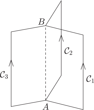
Figure 1: Three quark Wilson loop.

In the following we shall concentrate on abelian variables, referring to the maximally abelian gauge (MAG), and being obtained by standard abelian projection tHooft ; KLSW . To fix the MAG brand , we use a simulated annealing algorithm described in zeroT . We write the abelian link variables as

$$\begin{split}u(s,\mu)&\equiv{\rm diag}\big{(}u_{1}(s,\mu),u_{2}(s,\mu),u_{3}(s,\mu)\big{)}\,,\\[5.0pt] u_{i}(s,\mu)&=\exp({\rm i}\,\theta_{i}(s,\mu))\end{split}$$ (5)

with

$$\begin{split}\theta_{i}(s,\mu)&=\arg(U_{ii}(s,\mu))-\frac{1}{3}\sum_{j=1}^{3}\arg(U_{jj}(s,\mu))\,\big{|}_{\,{\rm mod}\ 2\pi}\,,\\ &\theta_{i}(s,\mu)\in[-\frac{4}{3}\pi,\frac{4}{3}\pi]\,.\end{split}$$ (6)

They take values in $U(1)\times U(1)$, and under a general gauge transformation they transform as

$$\begin{split}u(s,\mu)&\to d(s)^{\dagger}u(s,\mu)d(s+\hat{\mu})\,,\\ d(s)={\rm diag}\big{(}&\exp({\rm i}\,\alpha_{1}(s)),\exp({\rm i}\,\alpha_{2}(s)),\\ &\exp(-{\rm i}(\alpha_{1}(s)+\alpha_{2}(s)))\big{)}\,.\end{split}$$ (7)

The abelian Wilson loop is given by

$$W_{3Q}^{\rm ab}=\frac{1}{3!}\,|\varepsilon_{ijk}|u_{i}(\mathcal{C}_{1})u_{j}(\mathcal{C}_{2})u_{k}(\mathcal{C}_{3})\,,$$ (8)

where $u(\mathcal{C})$ is the abelian counterpart of (3). $W_{3Q}^{\rm ab}$ is invariant under gauge transformations (7).

The physical properties of the $3Q$ system can be infered from correlation functions of appropriate operators with the corresponding Wilson loop. Abelian operators take the form

$$\mathcal{O}(s)=\mbox{diag}(\mathcal{O}_{1}(s),\mathcal{O}_{2}(s),\mathcal{O}_{3}(s))\in U(1)\times U(1)\,.$$ (9)

For C-parity even operators $\mathcal{O}$, like the action and monopole densities, the correlator of $\mathcal{O}(s)$ with the abelian Wilson loop is given by bikk ; ibss

$$\langle\mathcal{O}(s)\rangle_{3Q}=\frac{\langle\mathcal{O}(s)W_{3Q}^{\rm ab}\rangle}{\langle W_{3Q}^{\rm ab}\rangle}-\langle\mathcal{O}\rangle\,.$$ (10)

For C-parity odd operators, like the electric field and monopole current which carry a color index, the correlator is defined by

$$\langle\mathcal{O}(s)\rangle_{3Q}=\frac{1}{3!}\frac{\langle\mathcal{O}_{i}(s)\,|\varepsilon_{ijk}|\,u_{i}(\mathcal{C}_{1})u_{j}(\mathcal{C}_{2})u_{k}(\mathcal{C}_{3})\rangle}{\langle W_{3Q}^{\rm ab}\rangle}\,,$$ (11)

where summation over $i,j,k$ is assumed. It is natural to use Wilson loop to study the static potential at zero temperature since it gives directly a singlet potential. The Polyakov loop correlator gives in general a color-averaged potential, i.e. a mixture of the singlet and octet potentials, see e.g. Nadkarni . At nonzero temperature one can use only the Polyakov loop correlator to study the static potential and we use the product $P_{3Q}$ of three Polyakov loops closed around the boundary as baryonic source instead of $W_{3Q}$:

$$P_{3Q}^{\rm ab}=\frac{1}{3!}\,|\varepsilon_{ijk}|\,\ell_{i}(\vec{s}_{1})\,\ell_{j}(\vec{s}_{2})\,\ell_{k}(\vec{s}_{3})\,,$$ (12)

where

$$\ell_{i}(\vec{s})=\prod_{s_{4}=1}^{L_{T}}u_{i}(\vec{s},s_{4},4)$$ (13)

is the abelian Polyakov loop, $L_{T}$ being the temporal extent of the lattice here. The correlators of $\mathcal{O}(s)$ with $P_{3Q}$ are defined analogously to (10) and (11).

The observables we shall study are the action density $\rho_{A}^{3Q}$, the color electric field $E^{3Q}$ and the monopole current $k^{3Q}$. The action density is given by

$$\rho_{A}^{3Q}(s)=\frac{\beta}{3}\sum_{i,\mu>\nu}\langle\cos(\theta_{i}(s,\mu,\nu))\rangle_{3Q}\,,$$ (14)

where

$$\theta_{i}(s,\mu,\nu)={\rm arg}(u_{i}(s,\mu,\nu))$$ ,

(15)

is the plaquette angle. The color electric field and monopole current correlators are defined by

$$E^{3Q}(s,i)={\rm i}\,\langle\mbox{diag}(\theta_{1}(s,4,i),\theta_{2}(s,4,i),\theta_{3}(s,4,i))\rangle_{3Q}$$ (16)

and

$$k^{3Q}(^{*}s,\mu)=2\pi{\rm i}\,\langle\mbox{diag}(k_{1}(^{*}s,\mu),k_{2}(^{*}s,\mu),k_{3}(^{*}s,\mu))\rangle_{3Q}\,,$$ (17)

where $k_{i}(^{*}s,\mu)$ is the monopole current bikk ; zeroT .

The calculations in full QCD at zero temperature are performed on the $24^{3}\,48$ lattice at $\beta=5.29$, $\kappa=0.1355$, which corresponds to a pion mass of $m_{\pi}/m_{\rho}\approx 0.7$ and a lattice spacing of $a/r_{0}=0.18$ zeroT (i.e. $a=0.09$ fm assuming $r_{0}=0.5$ fm). The calculations in full QCD at finite temperature $T$ are done on the $16^{3}\,8$ lattice at $\beta=5.2$ for various hopping parameters ranging from $\kappa=0.1330$ to $\kappa=0.1360$, which covers the temperature range finT $0.8\lesssim T/T_{c}\lesssim 1.2$. The critical temperature $T_{c}$ corresponds to $\kappa=0.1344(1)$. At this $\kappa$ we find $m_{\pi}/m_{\rho}\approx 0.77$. For comparison, we also did quenched simulations at zero temperature on the $16^{3}\,32$ lattice at $\beta=6.0$. At this $\beta$ the lattice spacing is $a/r_{0}=0.186$, i.e. it is roughly the same as on our full QCD lattices. To reduce the statistical noise we smeared the spatial links of the abelian Wilson loop using 10 sweeps of APE smearing Albanese:ds with $\alpha=2$, where $\alpha$ is a coefficient multiplying the sum of staples.

III Static potential and baryonic flux at zero temperature

The minimal Y-type distance between the quarks, i.e. the sum of the distance from the quarks to the Fermat point is tmns

$$L_{\sf Y}=\left(\frac{1}{2}\sum_{i>j}\,r_{ij}^{2}+2\sqrt{3}\,S_{\Delta}\right)^{1/2},$$ (18)

where $\vec{r}_{i}$ marks the position of the $i^{\rm th}$ quark, $r_{ij}=|\vec{r}_{i}-\vec{r}_{j}|$ and $S_{\Delta}$ is the area of the triangle spanned by the three quarks. The $Y$–Ansatz predicts that the confining part of the baryonic potential is $\sigma^{3Q}_{Y}L_{Y}$, with string tension $\sigma^{3Q}_{Y}$ equal to the $Q\bar{Q}$ string tension Carlson:1982xi :

$$\sigma^{3Q}_{Y}=\sigma^{Q\bar{Q}}.$$ (19)

The full expression describing both large and small distances is

$$V^{3Q}(L_{Y})=V_{0}^{3Q}-\sum_{i<j}\frac{\alpha^{3Q}}{r_{ij}}+\sigma^{3Q}_{Y}L_{Y}\,,$$ (20)

where, similarly to the $Q\bar{Q}$ static potential, $V_{0}^{3Q}$ is a selfenergy term, the Coulomb term with effective coupling $\alpha^{3Q}$ comprises one gluon exchange as well as a Lüscher term, recently derived for the baryonic string in Jahn:2003uz , and the confining term has string tension $\sigma^{3Q}_{Y}$. The $\Delta$–Ansatz prediction Cornwall:1996xr is that the confining part of the potential is proportional to the perimeter of the triangle formed by the quarks

$$L_{\Delta}=\sum_{i<j}|\vec{r}_{i}-\vec{r}_{j}|\,.$$ (21)

with string tension

$$\sigma^{3Q}_{\Delta}=\frac{1}{2}\sigma^{Q\bar{Q}}\,.$$ (22)

The short distance part is of the same form as in eq.(20). Thus the full expression for the $\Delta$–Ansatz potential is

$$V^{3Q}(L_{\Delta})=V_{0}^{3Q}-\sum_{i<j}\frac{\alpha^{3Q}}{r_{ij}}+\sigma^{3Q}_{\Delta}L_{\Delta}\,.$$ (23)

For short distances perturbation theory arguments relate the selfenergy and the Coulomb term coefficient to those of the $Q\bar{Q}$ static potential afj :

$$V_{0}^{3Q}=\frac{3}{2}V_{0}^{Q\bar{Q}}\,,\,\,\,\,\alpha^{3Q}=\frac{1}{2}\alpha^{Q\bar{Q}}\,.$$ (24)

On the other hand fitting the numerical data including both long and short distances by (20) or by (23) one may find results which differ from (24), e.g. due to the Lüscher term contribution. In Ref.tmns a rough agreement between the fit parameters and (24) has been found for both $Y$–Ansatz and $\Delta$–Ansatz fits.

Figure 2: The abelian baryon potential in full and quenched QCD.

Figure 3: Comparison of the abelian and SU(3) baryon potential in the quenched approximation on the $16^{3}\,32$ lattice at $\beta=6.0$. The SU(3) potential is taken from tmns .

In Fig.2 we show the baryon potential as a function of $L_{Y}$. An unphysical constant $V^{3Q}_{0}$ has been subtracted from the potentials. For equal distances between the quarks, i.e. $|\vec{r}_{i}-\vec{r}_{j}|\equiv d=L_{\sf Y}/\sqrt{3}$ for $\forall\,i\neq j$, eq.(20) becomes

$$V^{3Q}(L_{\sf Y})=V_{0}^{3Q}-3\sqrt{3}\frac{\alpha^{3Q}}{L_{\sf Y}}+\sigma^{3Q}_{Y}L_{\sf Y}\,.$$ (25)

Fitting our data for three quarks in equilateral triangles by eq.(25) for distances $d<0.75$ fm we found the abelian string tension $\sigma^{3Q}_{Y,\rm ab}\,a^{2}=0.038(1)$ and 0.0395(12) for the quenched and full theory, respectively. These values agree within error bars with the abelian string tension for the $Q\bar{Q}$ flux tube $\sigma_{\rm ab}^{Q\bar{Q}}=0.039(1)$ and 0.0402(11) zeroT thus supporting the $Y$–Ansatz. Note, that both $3Q$ and $Q\bar{Q}$ abelian string tensions are slightly higher in full QCD. We found values for the selfenergy and the Coulomb term coefficient smaller than prescribed by (24): $V_{0}^{3Q}/V_{0}^{Q\bar{Q}}=1.28(5),\,\alpha^{3Q}/\alpha^{Q\bar{Q}}=0.27(4)$ in full QCD and $V_{0}^{3Q}/V_{0}^{Q\bar{Q}}=1.31(6),\,\alpha^{3Q}/\alpha^{Q\bar{Q}}=0.31(4)$ in quenched QCD. The fits are also shown in Fig.2.

In Fig.3 the abelian and the nonabelian quenched potentials are plotted together with respective fits. The data for the nonabelian potential is taken from Ref. tmns . Comparison of $\sigma^{3Q}_{Y,\rm ab}$ with the SU(3) result tmns gives $\sigma^{3Q}_{Y,\rm ab}/\sigma^{3Q}_{Y}=0.83(3)$, which lends further support to the hypothesis of abelian dominance.

Figure 4: The abelian baryon potential in full QCD, together with its monopole and photon part, as a function of $L_{\sf Y}$ (top) and $L_{\Delta}$ (bottom), respectively. The curves show fits (25) (top) and (23) (bottom) to the data with equal distances between the static sources.

If the confining flux is of Y-shape we would expect the long-distance part of the potential to be a universal function of $L_{\sf Y}$. In Fig.4 we plot the abelian potential as a function of $L_{\sf Y}$ (top), and as a function of $L_{\Delta}$ (bottom). The data show a universal behavior when plotted against $L_{\sf Y}$. This is to a lesser extent the case when plotted against $L_{\Delta}$, which supports a genuine three-body force of Y-type. In Fig.4 the fits by the $Y$–Ansatz and by the $\Delta$–Ansatz for the quarks in the equilateral triangle are shown in the top and bottom parts, respectively. Note that for the quarks in the equilateral triangle these two fits are essentially the same with $\sigma^{3Q}_{\Delta}=\frac{1}{\sqrt{3}}\sigma^{3Q}_{Y}$ and equal selfenergy and Coulomb coefficient.

Figure 5: The abelian three-quark potential and $\Delta$ and $Y$–Ansätze in full QCD for quarks in equilateral triangles as function of quark separation $d=L_{Y}/\sqrt{3}=L_{\Delta}/3$. The solid line is a fit to the data, the dotted line is the $\Delta$–Ansatz prediction eq. (23) and the dashed line is the $Y$–Ansatz prediction eq.(25). For both Ansätze eq.(24) was used.

Figure 6: Same as Fig.5 for quenched QCD.

In Fig.5 and Fig.6 we show further comparison of our data with $\Delta$ and $Y$–Ansätze for full and quenched QCD. The data for the three-quark potential are plotted as a function of distance $d$ for equilateral triangle. In the same figures the curves showing respective $Y$–Ansatz and $\Delta$–Ansatz predictions are plotted. We fix all parameters in the Ansätze using relations (19), (22) and (24). We see that for both full and quenched QCD at distances $d<0.5$ fm the three quark potential data agree with the $\Delta$–Ansatz, while at larger distances it agrees with $Y$–Ansatz up to an additive constant indicating that the string tension $\sigma^{3Q}_{Y,\rm ab}$ is equal to $\sigma^{Q\bar{Q}}_{\rm ab}$ as was already discussed above. Similar findings were presented for the quenched nonabelian potential in aft . Thus we conclude that our data for the abelian potential confirm the $Y$–Ansatz for large distances. The agreement with the $\Delta$–Ansatz at short distances, which was also observed in aft , is probably a coincidence since the $\Delta$–Ansatz prediction eq.(22) is formulated for large quark separations. On the other hand, the proximity of the potential to the $\Delta$–Ansatz at distances which are relevant for the spectrum calculations might be important for the phenomenologists since the calculations with the $\Delta$–Ansatz potential are much simpler. The disagreement with the Y-Anzatz at small distances was first clearly observed in Ref.afj . One can guess that the finite size of the junction play the role in appearance of this discrepancy. Although our data for the static potential at small distances behave similar to that of Ref.afj we are not in a position to make strong statements about the short distances since we are using the abelian projection which, as many earlier observations suggest, gives correct description of the static potentials at large distances only.

Figure 7: Distribution of the color electric field $\vec{E}^{3Q}$ in the $(x,y)$ plane on the $24^{3}\,48$ lattice (center bottom figure), together with the monopole currents $k^{3Q}$ in the $(x,z)$ and $(y,z)$ planes (adjacent figures), respectively, at the position marked by the respective solid lines. The magnitude of $E^{3Q}$ and $k^{3Q}$ is indicated by the length of the arrows.

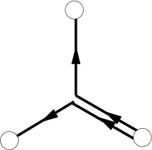
Figure 8: Schematic view of the color electric field.

Although the results for the static potential are in favor of the $Y$–Ansatz, the difference from the $\Delta$–Ansatz prediction is rather small. Thus it is worthwhile to study the color flux distribution. In Fig.7 we show the distribution of the color electric field $\vec{E}^{3Q}$, and its surrounding monopole currents $k^{3Q}$, on the $24^{3}\,48$ lattice in full QCD. The time direction of the Wilson loop has been taken in one of the spatial directions of the lattice. Points on the hyperplane orthogonal to the time direction of the Wilson loop are marked by $(x,y,z)$. The static quarks are placed at $(x,y,z)=(20,10,8)$, $(25,18,8)$ and $(30,10,8)$, respectively, i.e. they lie in the $(x,y)$ plane. The color index of the electric field operator (cf. eq. (16)) is identified with the color index of the quark in the bottom-right corner (in the center bottom figure). Note that the sum of the electric field over the three color indices vanishes at any point. As expected, the flux emanates from the quark in the bottom-right corner and at about the center of the $3Q$ system splits into two parts. The flux lines are schematically drawn in Fig.8. A similar picture holds for the top and bottom-left quark and their respective fluxes. In the adjacent figures we show the monopole current in the planes perpendicular to the electric flux lines, i.e. the $(x,z)$ and $(y,z)$ planes. They form a solenoidal current, as in the case of the $Q\bar{Q}$ system, in agreement with the dual superconductor picture of confinement.

We may decompose the abelian gauge field into a monopole and photon part according to the definition Smit ; Suzuki

$$\theta_{i}(s,\mu)=\theta_{i}^{\rm mon}(s,\mu)+\theta_{i}^{\rm ph}(s,\mu)$$ ,

 ,

(26)

where $D(s)=\Delta^{-1}(s)$ is the lattice Coulomb propagator, $\nabla^{(-)}_{\mu}$ is the lattice backward derivative, and $m_{i}(s,\mu,\nu)$ counts the number of Dirac strings piercing the plaquette $u_{i}(s,\mu,\nu)$. If one computes $k_{i}(^{*}s,\mu)$ from $\theta_{i}^{\rm mon}(s,\mu)$ one recovers almost all monopole currents. In Fig.4 we see that the monopole part is largely responsible for the linear behavior of the potential, as was found already in case of the $Q\bar{Q}$ potential zeroT . The ratio of monopole to abelian string tension turns out to be 0.81(3).

In Fig.9 we show the distribution of the abelian color electric field photon parts. The photon part shows a Coulomb-like distribution, while the monopole part has no sources. Outside the flux tube the monopole and photon parts of the color electric field largely cancel. The middle figure shows clearly that the flux lines are attracted to a Y-type geometry.

In Fig.10 we show the action density $\rho_{A}^{3Q}$ of the $3Q$ system in full QCD. Also shown is the monopole and photon part of $\rho_{A}^{3Q}$ separately. Let us first look at the (full) abelian density. It clearly displays a Y-type geometry of the color forces. This is, of course, indistinguishable from a geometry of purely two-body forces with strongly attracting flux lines. The monopole part of the action density shows no sources. Apart from that, it appears that the action density originates almost entirely from the monopole part. The sources show up in the photon part of the action density as expected.

Figure 9: Distribution of the abelian color electric field $\vec{E}^{3Q}$ (top) broken into monopole (middle) and photon parts (bottom) on the $24^{3}\,48$ lattice in full QCD. The color index of the electric field operators corresponds to that of the quark in the bottom right corner. Only part of the lattice is shown here.

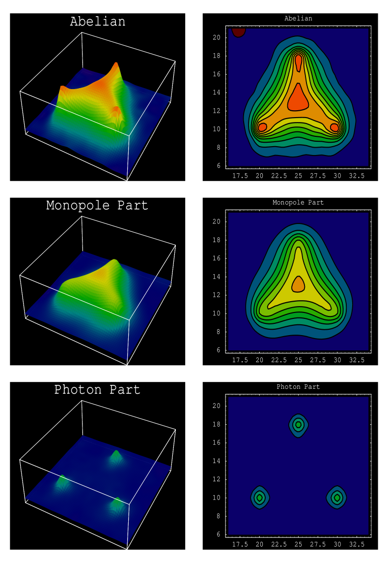
Figure 10: The abelian action density of the $3Q$ system in full QCD, together with the monopole and photon part.

We have done similar calculations (to the ones shown in Figs.4, 7, 9, 10) in quenched QCD as well. Part of our findings have been reported in ibss , and we refrain from repeating them here. Qualitatively, we found the same results as in full QCD at $m_{\pi}/m_{\rho}\approx 0.7$. In Fig. 11 we compare the action density of full and quenched QCD. We see that at the center of the flux tube the action density in full QCD is slightly higher than for the quenched case, while the shapes are rather similar. The same feature has been observed for the $Q\bar{Q}$ flux tube zeroT . We have estimated the width $\delta$ of the flux tube using a Gaussian fit zeroT . The result is $\delta=0.30(4)$ fm and $0.36(11)$ fm in full and quenched QCD, respectively. This is to be compared with the width of the $Q\bar{Q}$ flux tube, which turned out to be 0.29(1) fm in full and quenched QCD zeroT . We found that the width increases closer to the junction. So the numbers quoted above are only to tell that the width of the baryon flux tube, away from the junction is not very different from that of the $Q\bar{Q}$ flux tube. For a more precise determination of the width larger quark separation is necessary.

Figure 11: The action density $\rho_{A}^{3Q}r_{0}^{4}$ of Fig. 10 plotted across the flux tube at the distance $3a$ from the quark and $2a$ from the junction.

It is interesting to compare the action density shown in Fig. 10 with the action density constructed out of three $Q\bar{Q}$ flux tube action densities multiplied, in agreement with (22), by a factor $\frac{1}{2}$ to take into account that we are dealing with pairs of quarks rather than with $Q\bar{Q}$ pairs. Such a comparison has been done in Ref.afj for the Potts model. For the $Q\bar{Q}$ action density we used the results of Ref.zeroT . The resulting density is shown in Fig. 12. Figures 10 and 12 look rather different. The most important difference is that the measured density has a bump in the center, while the $\Delta$–Ansatz density has a dip. This comparison gives further support to the $Y$–Ansatz.

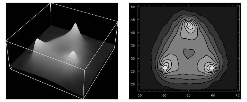
Figure 12: The abelian action density of the $3Q$ system as predicted by the $\Delta$–Ansatz in full QCD.

IV Baryonic flux at finite temperature

We expect the flux tube to disappear and the color electric field to become Coulomb- or Yukawa-like above the finite temperature phase transition $T_{c}$ and when the string breaks in full QCD. This phenomenon has been observed in case of the $Q\bar{Q}$ system in the pure SU(2) gauge theory for temperatures $T>T_{c}$ hay2 and in full QCD for $T$ just below and above $T_{c}$ bikm . Throughout this Section we shall use the Polyakov loop (12) to create a baryon.

In Fig.13 we show the baryon potential on the $16^{3}\,8$ lattice at $\beta=5.2$ for several values of $\kappa$. At this $\beta$ value

$$T\propto\exp(-2.81/\kappa)\,.$$ (27)

Increasing $\kappa$ thus increases the temperature. We cross the finite temperature phase transition at $\kappa=0.1344$ finT . We see that the potential flattens off while we approach the transition point. However, the distances we were able to probe are not large enough to make any statement about string breaking.

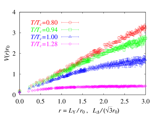
Figure 13: The monopole part of the baryon potential at finite temperature in full QCD as a function of $L_{\sf Y}$ ($T\leq T_{c}$) and $L_{\Delta}$ ($T>T_{c}$), respectively.

To compute the action density $\rho_{A}^{3Q}$ and the electric field and monopole correlators $E^{3Q}$ and $k^{3Q}$, respectively, we need to reduce the statistical noise. We do that by averaging over time slices and using extended operators

$$\begin{split}\rho_{A}^{3Q}(s)&\longrightarrow\\ &\frac{1}{8}\{\rho_{A}^{3Q}(s)+\rho_{A}^{3Q}(s-\hat{1}-\hat{2}-\hat{3})+\rho_{A}^{3Q}(s-\hat{1}-\hat{2})\\ &+\rho_{A}^{3Q}\big{(}s-\hat{1}-\hat{3})+\rho_{A}^{3Q}(s-\hat{2}-\hat{3})+\rho_{A}^{3Q}(s-\hat{1})\\ &+\rho_{A}^{3Q}(s-\hat{2})+\rho_{A}^{3Q}(s-\hat{3})\}\,,\end{split}$$ (28)

$$E^{3Q}(s,i)\longrightarrow\frac{1}{2}\{E^{3Q}(s,i)+E^{3Q}(s-\hat{i},i)\}\,,$$ (29)

$$k^{3Q}(^{*}s,\mu)\longrightarrow\frac{1}{2}\{k^{3Q}(^{*}s,\mu)+k^{3Q}(^{*}(s-\hat{\rm 2}),\mu)\}\,,\,\mu=1,3$$ (30)

where (again) we have assumed that the quarks lie in the $(x,y)$ plane, and we consider the monopole current in the $(z,x)$ plane.

In Fig.14 we plot the abelian action density in the deconfined phase at $\kappa=0.1360$. As was to be expected, the action density shows three Coulomb-like peaks at the position of the quarks, similar to the photon part of the action density at zero temperature as shown in Fig.10.

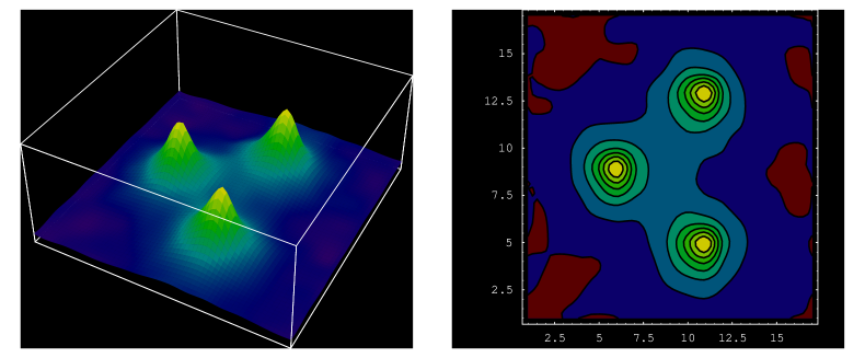
Figure 14: The Abelian action density in the deconfined phase at $\kappa=0.1360$.

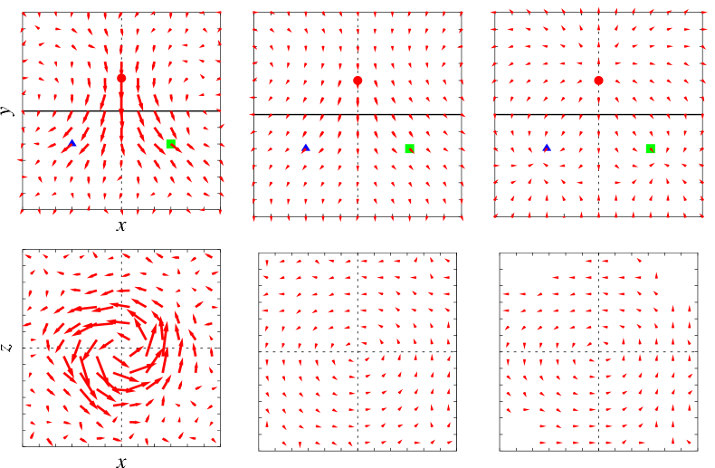
Figure 15: The color electric field (top) and monopole currents (bottom) on the $16^{3}\,8$ lattice at $\kappa=0.1335$ (left), $0.1344$ (middle) and $0.1360$ (right). The three quarks lie in (what we call) the $(x,y)$ plane. The bottom figures show the monopole currents in the $(x,z)$ plane at the position marked by the solid lines in the top figures.

In Fig.15 we show the monopole part of the electric field, averaged over the color components, and the accompanying monopole current for three values of $\kappa$, corresponding (from left to right) to the confined case, to $T\approx T_{c}$ and to the deconfined phase. In the confinement phase ($\kappa=0.1335$) we find the flux to be of Y-shape, similar to the zero temperature case where we used Wilson loop correlators. Note that the Polyakov lines do not have a Y-shape junction like the Wilson loop does, which excludes the possibility that the flux is being induced by the color lines. Just below $T_{c}$ ($\kappa=0.1344$) we still see a Y-shape flux, while in the deconfined phase ($\kappa=0.1360$) the electric field becomes Coulomb-like.

V Conclusions

We have studied the $3Q$ system in the maximally abelian gauge in full QCD at zero and at finite temperature. Among the quantities we have looked at are the abelian baryon potential as well as the flux distribution and the action density. While on the basis of the potential it is hard to decide whether the long-range potential is of $\Delta$- or Y-type, the distribution of the color electric field and the action density clearly shows a Y-shape geometry. As in the $Q\bar{Q}$ system, we identified the solenoidal monopole current to be responsible for squeezing the color electric flux into a narrow tube. Little difference to the quenched theory was found. In the deconfined phase the flux tube disappears, and the color electric field assumes a Coulomb-like form. Our results are in qualitative agreement with the predictions of the dual Ginzburg-Landau model Koma : the baryon flux has $Y$-shape, and the solenoidal monopole currents are clearly observed.

References

- (1) S. Capstick and N. Isgur, Phys. Rev. D 34, 2809 (1986).
- (2) G.S. Bali, Phys. Rept. 343, 1 (2001).
- (3) C. Alexandrou, Ph. de Forcrand and A. Tsapalis, Phys. Rev. D 65, 054503 (2002).
- (4) T.T. Takahashi, H. Suganuma, Y. Nemoto and H. Matsufuru, Phys. Rev. D 65, 114509 (2002); T.T. Takahashi, H. Matsufuru, Y. Nemoto and H. Suganuma, Phys. Rev. Lett. 86, 18 (2001).
- (5) C. Alexandrou, Ph. de Forcrand and O. Jahn, Nucl. Phys. Proc. Suppl. 119, 667 (2003).
- (6) D.S. Kuzmenko and Yu.A. Simonov, Phys. Lett. B494 (2000) 81; Phys. Atom. Nucl. 67, 543 (2004) [Yad. Fiz. 67, 561 (2004)].
- (7) H. Ichie, V. Bornyakov, T. Streuer and G. Schierholz, Nucl. Phys. Proc. Suppl. 119, 751 (2003); H. Ichie, V. Bornyakov, T. Streuer and G. Schierholz, Nucl. Phys. A 721, 899 (2003).
- (8) H. Stüben, Nucl. Phys. Proc. Suppl. 94, 273 (2001).
- (9) S. Nadkarni, Phys. Rev. D 33, 3738 (1986).
- (10) V.G. Bornyakov, H. Ichie, Y. Koma, Y. Mori, Y. Nakamura, D. Pleiter, M.I. Polikarpov, G. Schierholz, T. Streuer, H. Stüben and T. Suzuki, hep-lat/0310011.
- (11) G. ’t Hooft, Nucl. Phys. B 190, 455 (1981).
- (12) A.S. Kronfeld, M.L. Laursen, G. Schierholz and U.-J. Wiese, Phys. Lett. B 198, 516 (1987).
- (13) F. Brandstaeter, G. Schierholz and U.-J. Wiese, Phys. Lett. B 272, 319 (1991).
- (14) V. Bornyakov, H. Ichie, S. Kitahara, Y. Koma, Y. Mori, Y. Nakamura, M. Polikarpov, G. Schierholz, T. Streuer, H. Stüben and T. Suzuki, Nucl. Phys. Proc. Suppl. 106, 634 (2002).
- (15) V.G. Bornyakov, M.N. Chernodub, H. Ichie, Y. Koma, Y. Mori, Y. Nakamura, M.I. Polikarpov, G. Schierholz, A. Slavnov, H. Stüben, T. Suzuki, P. Uvarov and V.I. Veselov, hep-lat/040101403.
- (16) M. Albanese et al. [APE Collaboration], Phys. Lett. B 192, 163 (1987).
- (17) J. Carlson, J. B. Kogut and V. R. Pandharipande, Phys. Rev. D 27, 233 (1983).
- (18) O. Jahn and P. de Forcrand, Nucl. Phys. Proc. Suppl. 129-130, 700 (2004).
- (19) J. M. Cornwall, Phys. Rev. D 54, 6527 (1996).
- (20) J. Smit and A. van der Sijs, Nucl. Phys. B 355, 603 (1991).
- (21) T. Suzuki, S. Ilyar, Y. Matsubara, T. Okude and K.Yotsuji, Phys. Lett. B 347, 375 (1995); [Erratum-ibid. B 351, 603 (1995)].
- (22) Y. Peng and R.W. Haymaker, Phys. Rev. D 52, 3030 (1995).
- (23) V. Bornyakov, H. Ichie, Y.Koma, Y. Mori, Y. Nakamura, M. Polikarpov, G. Schierholz, T. Streuer and T. Suzuki, Nucl. Phys. Proc. Suppl. 119, 712 (2003).
- (24) M. N. Chernodub and D. A. Komarov, JETP Lett. 68, 117 (1998); Y. Koma, E.-M. Ilgenfritz, T. Suzuki, H. Toki, Phys. Rev. D 64, 014015 (2001).