.

DFCAL-TH 04/1

January 2004

Real and imaginary chemical potential in 2-color QCD

P. Giudice and A. Papa

Dipartimento di Fisica, Università della Calabria

& Istituto Nazionale di Fisica Nucleare, Gruppo collegato di Cosenza

I-87036 Arcavacata di Rende, Cosenza, Italy

e-mail address: giudice, papa@cs.infn.it

In this paper we study the finite temperature SU(2) gauge theory with staggered fermions for non-zero imaginary and real chemical potential. The method of analytical continuation of Monte Carlo results from imaginary to real chemical potential is tested by comparison with simulations performed directly for real chemical potential. We discuss the applicability of the method in the different regions of the phase diagram in the temperature – imaginary chemical potential plane.

 

1 Introduction

Understanding the QCD phase diagram in the temperature – chemical potential ($T,\mu$) plane has many important implications in cosmology, in astrophysics and in the phenomenology of heavy-ion collisions (for a review, see [1]). In particular, it is extremely important to localize with high accuracy the critical lines in this plane and to determine if the transition across them is first order, second order or just a crossover [2].

The formulation of the theory on a space-time lattice offers a unique tool for such task. However, at non-zero chemical potential the determinant of the fermion matrix becomes complex, thus preventing to perform standard Monte Carlo simulations. One way out is to take advantage of physical fluctuations in the thermal ensemble generated at $\mu=0$ in order to extract from it information at (small) non-zero $\mu$, after suitable reweighting [3, 4, 5, 6]. However, it is not possible to know a priori to what extent the reweighted ensemble overlaps the true one at non-zero $\mu$.

An alternative approach is based on the idea to perform numerical simulations at imaginary chemical potential [8], for which the fermion determinant is again real, and to analytically continue the results to real $\mu$ [9, 10, 11, 12, 13]. In practice, the method consists in fitting the numerical data obtained for imaginary chemical potential $\mu=i\mu_{I}$ by a polynomial, which is then prolongated to real $\mu$. The advantage of this method lies in the fact that its applicability is not restricted by large lattice volumes, since it makes no use of reweighting. Therefore, size scaling analysis can be made after the analytical continuation to clarify the nature of the transition across the critical lines. On the other side, a limitation comes from the presence of non-analyticities in $\mu$, thus implying, as we will see later on, that the method works practically only for $\mu\lesssim T$.

In particular, if non-analyticities are singled out for imaginary $\mu$ and even if numerical data are obtained inside a region of analyticity in the $(T,\mu_{I})$ plane, it is necessary that during the “rotation” from $\mu=i\mu_{I}$ to real $\mu=\mu_{R}$ no other non-analyticities are met. It is understood that non-analyticities show up only in the infinite volume limit and that all observables are analytic on finite lattices. However, the presence of non-analyticities in the thermodynamical limit is indicated on (large) finite volumes by sharp changes in the behavior of physical observables, which is practically difficult to interpolate by polynomials, if not by including a large number of terms. The papers where the method of analytical continuation has been used so far limited the attention to regions of temperature and chemical potential where this situation does not occur.

Of course, the compatibility between the results from two very different approaches, such as reweighting and analytical continuation, would give reasonable confidence on the validity of both. Such consistency has been shown in the case of 4-flavor QCD in Ref. [11].

Nevertheless, a test of both methods by comparison with direct determinations from standard Monte Carlo is interesting, especially because it could shed light also on the applicability outside the regions usually considered in literature. For this purpose, it is necessary to turn to a theory where direct Monte Carlo simulations in presence of real chemical potential are feasible.

It is well known that the determinant of the fermion matrix of 2-color QCD or SU(2) gauge theory is real even in presence of a real chemical potential (see, for instance [8]). Moreover, although being very different in the structure of the spectrum [15], 2-color QCD shares many similarities with true QCD, therefore represents the best candidate for the mentioned test.

In this paper we adopt 2-color QCD to compare determinations of the Polyakov loop and of the chiral condensate from the method of analytical continuation with results from direct Monte Carlo simulations. In particular, we characterize different regions of the phase diagram in the $(T,\mu_{I})$ plane according to the applicability of this method. Our findings can be helpful to apply and to understand the results of the method of analytical continuation in the theory of physical interest, i.e. in true QCD.

The paper is organized as follows: in Section 2 we describe the structure of the phase diagram of 2-color QCD in the $(T,\mu_{I})$ plane and discuss the implications on the method of analytical continuation; in Section 3 we present the numerical results; in Section 4 we draw some conclusions and anticipate some future developments.

2 The phase diagram of 2-color QCD

In order to draw the phase diagram of 2-color QCD we make use of known theoretical and numerical results on the behavior with temperature and chemical potential of the Polyakov loop $L$ and of the chiral condensate $\langle\bar{\psi}\psi\rangle$. These objects represent true order parameters only in two limiting cases: the Polyakov loop is the order parameter of the confinement-deconfinement transition in the limit of infinite quark masses, while the chiral condensate is that of the chiral transition in the limit of vanishing quark masses. However, there is a broad numerical evidence that they both exhibit a rapid variation in correspondence of certain values of the parameters of the theory, which therefore are taken as critical ones.

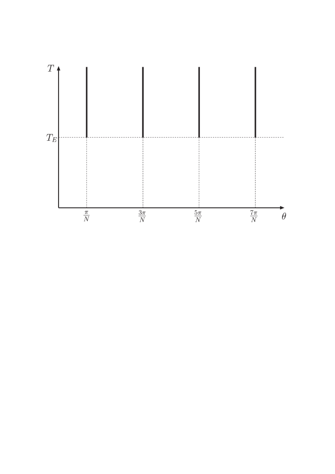
Figure 1: Schematization of the phase diagram in the $(T,\theta)$ plane according to Roberge and Weiss [16].

We start the discussion from the case of imaginary chemical potential, $\mu=i\mu_{I}$. Roberge and Weiss have shown [16] that the partition function of any SU(N) theory is periodic in the parameter $\theta=\mu_{I}/T$ (the Boltzmann constant is set equal to one) as consequence of a remnant of the Z(N) symmetry valid in absence of fermions. Moreover, they have shown by weak coupling perturbation theory that above a certain temperature $T_{E}$ the free energy and the Polyakov loop show cusps or discontinuities for $\theta=2\pi(k+1/2)/N$, with $k=0,1,\ldots$. This suggests that there are first order vertical critical lines in the $(T,\theta)$ plane located at $\theta=2\pi(k+1/2)/N$ and extending from $T_{E}$ to infinity (see Fig. 1). They argue also that below $T_{E}$, there is no phase transition for any value of $\theta$, this being true also in the physical case of $\theta=\mu=0$.

The latter conclusion cannot be true for all values of $n_{f}$ and of the fermion masses. In the chiral limit of QCD, there are arguments [17] according to which a chiral phase transition for $\mu=0$ does exist and is first order for $n_{f}\geq 3$ and second order for $n_{f}=2$. For SU(2), where a strong coupling analysis could be applied, according to Ref. [18] there is a second order chiral phase transition for $n_{f}=1$ and $n_{f}=2$. For non-vanishing masses, this phase transition probably becomes a crossover. Furthermore, a numerical study on a $12^{3}\times 4$ lattice in SU(2) with $n_{f}=8$ and $am=0.07$ has shown a peak in the susceptibility of the chiral condensate at $\beta_{c}\simeq 1.41$, suggesting the possibility of a chiral phase transition near this point [19].

In view of all this, the worst case for the purposes of the analytical continuation (but the most interesting from the point of view of the present study) is that the Roberge-Weiss (RW) critical line at $\theta=\pi/N$ could be prolongated downwards and bent up to reaching the $\theta=0$ axis in correspondence of a critical temperature $T_{c}$ (see also [11, 12]). For the reasons mentioned above, this prolongation of the RW critical line will be referred to in the following as the chiral critical line [11, 12]. The RW periodicity and the symmetry for $\mu\to-\mu$, resulting from CP invariance, imply that knowing the expectation value of an observable for $T$ and $\theta$ inside the strip $\{0\leq\theta\leq\pi/N,\;0\leq T<\infty\}$ in the $(T,\theta)$ plane is enough to fix it on the remaining part of the plane. Applying this argument also to the critical lines, we end up with the qualitative structure of the phase diagram drawn in Fig. 2. The actual nature of the transition across the branches of the critical lines of Fig. 2 which lie below $T_{E}$ is to a large extent unknown. Other scenarios of phase diagrams are possible, depending on $n_{f}$ and on the fermion masses, such as, for instance, that where a chiral critical line emanating from $T_{c}$ ends somewhere before joining the vertical lines [13].

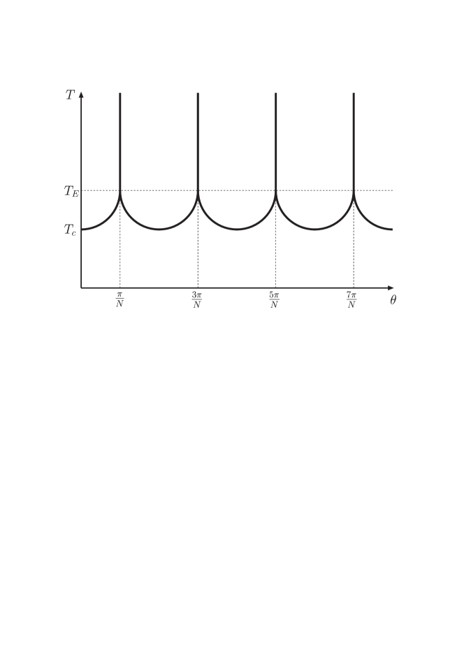
Figure 2: Schematization of the phase diagram in the $(T,\theta)$ plane after the inclusion of the chiral critical lines.

Inside the mentioned strip we can single out two regions where the (non-perturbative) determinations of an observable can be interpolated by a Taylor series in $\theta^{2}=(\mu_{I}/T)^{2}$: the region above and the region below the chiral critical line. This Taylor series can be analytically continued to real $\mu=\mu_{R}$ by the “rotation” $\mu_{I}\to-i\mu_{R}$, if no non-analyticities are met during this rotation. Such a condition is not a priori guaranteed. It is evident, that the crucial point is how the critical line in the $(T,\theta)$ plane, implicitely defined by $T=f(\mu_{I}/T)$, evolves during the rotation from imaginary to real $\mu$. A reasonable assumption is that, at the end of the rotation, the critical line in the plane with real $\mu$ is given by $T=f(-i\mu_{R}/T)\equiv g(\mu_{R}/T)$, with $g$ a monotonically decreasing function in $\mu_{R}/T$. Another assumption, which needs confirmation by numerical tests, is that the critical line evolves smoothly during the rotation, i.e. it spans in the $(T,\mu_{R}/T,\mu_{I}/T)$ space a 2-dimensional surface, connecting the critical line in the $(T,\mu_{I}/T)$ plane with the one in the $(T,\mu_{R}/T)$ plane, which does not possess bumps or ridges or valleys.

If these assumptions are true and the scenario of Fig. 2 holds, we can identify three regions in the strip $\{0\leq\theta\leq\pi/N,\;0\leq T<\infty\}$ of the $(T,\mu_{I}/T)$ plane according to the possibility to apply the analytical continuation:

• $T>T_{E}$: analytical continuation possible for $0\leq\mu_{I}/T<\pi/N$;

• $T_{c}<T<T_{E}$: analytical continuation possible for $0\leq\mu_{I}/T<\mu_{I}^{*}/T$, where $\mu_{I}^{*}/T$ is the solution of $T=f(\mu_{I}^{*}/T)$, i.e. the value of $\mu_{I}/T$ on the chiral critical line at the given temperature;

• $T<T_{c}$: analytical continuation possible for $0\leq\mu_{I}/T<-i\mu_{R}^{*}/T$, where $\mu_{R}^{*}/T$ is the solution of $T=g(\mu_{R}^{*}/T)$, i.e. the value of $\mu_{R}/T$ on the critical line of the $(T,\mu_{R}/T)$ plane at the given temperature.

So far the method of analytical continuation has been applied, implicitely making the assumptions we have mentioned, to the chiral condensate in the region $T>T_{E}$ for QCD with $n_{f}=4$ [11] and to the critical line itself for QCD with $n_{f}=4$ [11] and with $n_{f}=2,~{}3$ [13]. In the case of QCD with $n_{f}=4$, the analytically continued critical line has been found in agreement with the determination of Ref. [4].

In the next Section we will compare the scenario sketched in the above list with numerical simulations in all the three temperature regions. As a test-field theory we use 2-color QCD with $n_{f}=8$ and as observables we adopt the Polyakov loop $L$ and the chiral condensate $\langle\bar{\psi}\psi\rangle$.

3 Numerical results

We consider the formulation of 2-color QCD or SU(2) gauge theory on a $N_{\sigma}^{3}\times N_{\tau}$ lattice with staggered fermions for non-zero temperature and chemical potential of the baryonic density.

The finite temperature is realized by compactifying the time direction and by imposing (anti)periodic boundary conditions on (fermion) boson fields. The connection between the temperature $T$ and the lattice size in the time direction is $T=1/(N_{\tau}a)$, where $a=a(\beta)$ is the lattice spacing and $\beta\equiv 4/g^{2}$ is the bare coupling constant. The chemical potential is introduced by the replacements [20]

$$U_{\tau} \rightarrow e^{a\mu}\,U_{\tau}$$

$$U_{\tau}^{\dagger} \rightarrow e^{-a\mu}\,U_{\tau}^{\dagger}\;,$$ (1)

where $U_{\tau}$ and $U_{\tau}^{\dagger}$ are the gauge link variables in the forward and backward time direction, respectively. When $\mu$ is purely imaginary these replacements amount to add a constant background U(1) field to the original theory. For SU(2) the fermionic determinant, appearing in the partition function after integration of the fermion fields, is real for any complex value of the chemical potential $\mu$, thus allowing the Monte Carlo importance sampling without any limitation.

We adopted in this work the same hybrid simulation algorithm of Ref. [15]. Since for $\mu\neq 0$ it is not possible to use the even-odd partitioning, we were forced to simulate eight degenerate continuum flavors. We performed all the simulations on a $8^{3}\times 4$ lattice, setting the quark bare mass to $am=0.07$ and the microcanonical time step to $dt=0.02$. We made refreshments of the gauge fields every 5 steps of the molecular dynamics and of the pseudofermion fields every 3 steps. In order to reduce autocorrelation effects, we made “measurements” every 50 steps and analyzed data by the jackknife method combined with binning.

Before presenting the numerical results, it is convenient to redraw the phase diagram discussed in the previous Section in units more suitable for the lattice. In particular, on the vertical axis we put the inverse coupling $\beta$ which is connected to the temperature $T$ by a monotonic function in the region of interest (increasing $\beta$ means increasing temperature). On the horizontal axis we put the chemical potential in lattice units, $\hat{\mu}\equiv a\mu$. The qualitative structure of the phase diagrams in the $(\beta,\hat{\mu}_{I})$ and in the $(\beta,\hat{\mu}_{R})$ planes is the same as in the $(T,\mu_{I}/T)$ and in the $(T,\mu_{R}/T)$ planes. In the new units, however, the RW transition lines in the $(\beta,\hat{\mu}_{I})$ plane appear at $\hat{\mu}_{I}=2\pi(k+1/2)/(NN_{\tau})$. For $N=2$ the first RW transition line is located at $\hat{\mu}_{I}=\pi/(2N_{\tau})$. Of course, the scenario illustrated at the end of the previous Section must be reformulated in terms of $\beta$, $\beta_{E}$ and $\beta_{c}$.

An estimate of the value of $\beta_{c}$ can be deduced from the literature. Indeed, in Ref. [19], a study of the chiral condensate on a $12^{3}\times 4$ lattice for bare quark mass $am=0.07$ lead to the result $\beta_{c}=1.41\pm 0.03$. Since we have a different lattice, we expect a small difference between our $\beta_{c}$ and the determination of Ref. [19]. However, for our purposes we can safely adopt this value of $\beta_{c}$.

Figure 3: Polyakov loop (above) and chiral condensate (below) vs $\hat{\mu}_{I}$ for $\beta=1.80$ on a $8^{3}\times 4$ lattice. The solid vertical lines represent the first two RW critical lines ($\hat{\mu}_{I}=\pi/8$ and $\hat{\mu}_{I}=3\pi/8$).

As a first step we took two $\beta$ values, one (much) above $\beta_{c}$ and likely above $\beta_{E}$, the other below $\beta_{c}$ in order to possibly single out a different behavior in $\hat{\mu}_{I}$ of lattice observables across $\hat{\mu}_{I}=\pi/(2N_{\tau})$. We took $\beta$=1.80 for the higher $\beta$ value and $\beta=1.35$ for the lower and determined the Polyakov loop and the chiral condensate for $\hat{\mu}_{I}$ ranging between 0 and the value corresponding to the second RW critical line, i.e. $3\pi/(2N_{\tau})$. The results are shown in Figs. 3 and 4. We can clearly see the RW periodicity in all cases; however, for $\beta=1.80$ we have discontinuity for the Polyakov loop and cusp for the chiral condensate across the first RW critical line, while for $\beta=1.35$ the behavior is smooth for both observables. We have verified that the overshooting of the first RW critical line seen in Fig. 3 is due to an hysteresis effect, which confirms the first order nature of the transition.

Figure 4: As in Fig. 3 for $\beta=1.35$.

In order to proceed with the test of the method of analytical continuation we need also an estimation of $\beta_{E}$. There is a nice procedure to do it, suggested in Ref. [11]. It relies on performing simulations at a critical value of $\hat{\mu}_{I}$, say $\hat{\mu}_{I}=\pi/(2N_{\tau})$, and on changing $\beta$ from a very high value downwards. If the zero field configuration is chosen as the starting one, the system remains always in the phase on the left of the RW line until $\beta>\beta_{E}$, if the flip to the other phase is prevented by a large space volume. Due to our limited computational power, we are constrained to a space volume which is too small to prevent flips between the two phases. An alternative procedure to determine $\beta_{E}$ could be to study the behavior of the Polyakov loop (or of its phase) and of the chiral condensate across the RW critical lines for different $\beta$ values and to see when the discontinuities or the cusps are smoothed out. Another possibility could be to exploit the hysteresis effect in the Polyakov loop or in the chiral condensate determinations across the RW critical line. The procedure consists in building two sequences of expectation values of the Polyakov loop; in the first (second) sequence the starting configuration of any new run is taken to be a thermal equilibrium configuration being always in the phase on the left (right) side of the first RW transition. Across the RW critical line the comparison of these two sequences of data shows a hysteresis effect as long as $\beta>\beta_{E}$. This effect disappears below $\beta_{E}$. Of course, both the above procedures demand for a high statistics and, so far, we can only say that $\beta_{E}$ is bounded between about 1.53 and about 1.57. This level of accuracy is, however, enough for the purposes of the present study.

We turn now to the main part of this work, i.e. the test if the scenario presented at the end of the previous Section holds. We selected three values of $\beta$ (1.90, 1.45, 0.90), each representative of one of the regions $\beta>\beta_{E}$, $\beta_{c}<\beta<\beta_{E}$ and $\beta<\beta_{c}$. For each $\beta$ we have performed simulations for both real and imaginary chemical potential, varying $\hat{\mu}_{I}$ and $\hat{\mu}_{R}$ between 0 and $\pi/(2N_{\tau})$ and have determined expectation values of the Polyakov loop and of the chiral condensate. Then, we have interpolated the data obtained for imaginary $\mu$ with a truncated Taylor series of the form $a+b\,\hat{\mu}_{I}^{2}+c\,\hat{\mu}_{I}^{4}$. After “rotating” this polynomial to real chemical potential, thus leading to $a-b\,\hat{\mu}_{R}^{2}+c\,\hat{\mu}_{R}^{4}$, we have compared it with the determinations obtained directly for real $\mu=\mu_{R}$.

For $\beta=1.90$ we have interpolated with the fourth order polynomial the data obtained for $0\leq\hat{\mu}_{I}\lesssim\pi/(2N_{\tau})$ and have found that the rotated polynomial perfectly interpolates data obtained directly for real $\mu=\mu_{R}$ in the same range (see Fig. 5). The uncertainty in the rotated polynomial has been obtained by propagating in standard way the uncertainty on the fitted coefficients $a$, $b$ and $c$. We have verified that the same situation occurs for other values of $\beta$ larger than $\beta_{E}$. From this outcome we can conclude that the analytical continuation works in the region $\beta>\beta_{E}$ for all the $\hat{\mu}_{I}$’s before the first RW critical line.

Figure 5: Polyakov loop (above) and chiral condensate (below) vs $\hat{\mu}$ for $\beta=1.90$ on a $8^{3}\times 4$ lattice. Numerical data for imaginary chemical potential (squares) are fitted by a fourth order polynomial (long-dashed line). The “rotated” polynomial, whose upper and lower bounds are given by the solid lines, is compared with data obtained for real chemical potential (diamonds).

For $\beta=1.45$ we are in the region $\beta_{c}<\beta<\beta_{E}$ for which, if the scenario presented at the end of the previous Section holds, we expect that by varying $\hat{\mu}_{I}$ we meet the chiral critical line, while no transitions should be met at the same $\beta$ by varying $\hat{\mu}_{R}$. Therefore this time we have interpolated with the fourth order polynomial the data obtained for the real chemical potential $0\leq\hat{\mu}_{R}\lesssim\pi/(2N_{\tau})$ and have rotated this polynomial to its counterpart in $\hat{\mu}_{I}$. The comparison with data obtained directly for imaginary chemical potential shows agreement for $\hat{\mu}_{I}$ below $\simeq 0.18$, which can be taken as an estimate of the chiral critical value in the $(\beta,\hat{\mu}_{I})$ plane at the given $\beta$ (see Fig. 6).

Figure 6: Polyakov loop (above) and chiral condensate (below) vs $\hat{\mu}$ for $\beta=1.45$ on a $8^{3}\times 4$ lattice. Numerical data for real chemical potential (diamonds) are fitted by a fourth order polynomial (long-dashed line). The “rotated” polynomial, whose upper and lower bounds are given by the solid lines, is compared with data obtained for imaginary chemical potential (squares).

For $\beta=0.90<\beta_{c}$, we expect analyticity for all possible values of $\hat{\mu}_{I}$, while the chiral critical line in the $(\beta,\hat{\mu}_{R})$ plane is met by varying $\hat{\mu}_{R}$ at the given value of $\beta$. Therefore we have interpolated with the fourth order polynomial the data obtained for $0\leq\hat{\mu}_{I}\lesssim\pi/(2N_{\tau})$ and have rotated this polynomial to its counterpart in $\hat{\mu}_{R}$. The comparison with data obtained directly for real chemical potential shows agreement for $\hat{\mu}_{R}$ below $\simeq 0.12$, which can be taken as an estimate of the critical value in the $(\beta,\hat{\mu}_{R})$ plane at the given $\beta$ (see Fig. 7).

Figure 7: As in Fig. 5 for $\beta=0.90$.

We can conclude from these results that the scenario of the end of the previous Section is consistent, thus giving support to the assumptions underlying it.

4 Conclusions and outlook

In this paper we have presented a possible structure of the phase diagram in the temperature – imaginary chemical potential in 2-color QCD and have argued how this structure can be continued to real chemical potential. Then, we have shown that the scenario we have described is consistent with Monte Carlo numerical determinations of the Polyakov loop and of the chiral condensate for real and imaginary chemical potential.

In particular, we have found that the method of analytical continuation, largely exploited now in the literature for the physically interesting case of QCD, works fine within the restrictions posed by the presence of non-analyticities.

High precision determinations were not the aim of this paper. We limited ourselves to give convincing numerical support to the proposed scenario, postponing massive calculations to forthcoming works.

We plan, moreover, to further develop the present ideas by (a) determining the location of the critical lines for real and imaginary chemical potential by the standard method of susceptibilities, (b) verifying that the critical lines for real chemical potential can be obtained from analytical continuation of those for imaginary chemical potential, (c) following the “evolution” of the critical lines during the rotation from imaginary to real chemical potential by simulations with complex chemical potential.

Acknowledgments We have the pleasure to thank M.-P. Lombardo for many stimulating discussions and for providing us with the Monte Carlo code. We acknowledge also several interesting conversations with R. Fiore.

References

- [1] D. Boyanovsky, hep-ph/0102120.
- [2] S.D. Katz, hep-lat/0310051 and references therein.
- [3] I.M. Barbour, S.E. Morrison, E.G. Klepfish, J.B. Kogut, M.-P. Lombardo, Nucl. Phys. (Proc. Suppl.) 60A (1998) 220.
- [4] Z. Fodor and S.D. Katz, Phys. Lett. B534 (2002) 87; JHEP 0203 (2002) 014.
- [5] P.R. Crompton, Nucl. Phys. B619 (2001) 499.
- [6] S. Ejiri, hep-lat/0212022.
- [7] I. Barbour, S. Hands, J.B. Kogut, M.-P. Lombardo, S.E. Morrison, Nucl. Phys. B557 (1999) 327.
- [8] M.G. Alford, A. Kapustin, F. Wilczek, Phys. Rev. D59 (1999) 054502.
- [9] M.-P. Lombardo, Nucl. Phys. (Proc. Suppl.) 83 (2000) 375.
- [10] A. Hart, M. Laine and O. Philipsen, Phys. Lett. B505 (2001) 141.
- [11] M. D’Elia and M.-P. Lombardo, hep-lat/0205022; Phys. Rev. D67 (2003) 014505.
- [12] M. D’Elia and M.-P. Lombardo, hep-lat/0309114.
- [13] P. de Forcrand and O. Philipsen, Nucl. Phys. B642 (2002) 290; Nucl. Phys. (Proc. Suppl.) 119 (2003) 535; hep-ph/0301209; Nucl. Phys. B673 (2003) 170; hep-lat/0309109.
- [14] S. Gupta, hep-lat/0307007.
- [15] S. Hands, J.B. Kogut, M.-P. Lombardo, S.E. Morrison, Nucl. Phys. B558 (1999) 327.
- [16] A. Roberge and N. Weiss, Nucl. Phys. B275 (1986) 734.
- [17] R.D. Pisarski and F. Wilczek, Phys. Rev. D29 (1984) 338.
- [18] P.H. Damgaard, N. Kawamoto and K. Shigemoto, Nucl. Phys. B264 (1986) 1.
- [19] Y. Liu, O. Miyamura, A. Nakamura and T. Takaishi, hep-lat/0009009.
- [20] P. Hasenfratz and F. Karsch, Phys. Lett. B125 (1983) 308.