Non-perturbative calculation of $Z_{V}$ and $Z_{A}$ in domain-wall QCD on a finite box

Abstract

We report on a non-perturbative evaluation of the renormalization factors for the vector and axial-vector currents, $Z_{V}$ and $Z_{A}$, in the quenched domain-wall QCD (DWQCD) with plaquette and renormalization group improved gauge actions. We take the Dirichlet boundary condition for both gauge and domain-wall fermion fields on the finite box, and introduce the flavor-chiral Ward-Takahashi identities to calculate the renormalization factors. As a test of the method, we numerically confirm the expected relation that $Z_{V}\simeq Z_{A}$ in DWQCD. Employing two different box sizes for the numerical simulations at several values of the gauge coupling constant $g^{2}$ and the domain-wall height $M$, we extrapolate $Z_{V}$ to the infinite volume to remove $a/L$ errors. We finally give the interpolation formula of $Z_{V}$ in the infinite volume as a function of $g^{2}$ and $M$.

I Introduction

Recent lattice calculations in the domain-wall QCD (DWQCD) have shown that the good chiral property of domain-wall fermions leads to a good scaling behavior of physical observables such as quark masses and $B_{K}$cppacs_bk . Aside from the quenched approximation, the use of perturbative renormalization factors is the largest source of the uncontrolled systematic errors in these calculations. Some kind of the non-perturbative renormalization is required to reduce the total error to a few percent level except that from the quenched approximation.

There exist two popular methods for the non-perturbative renormalization in lattice QCD: one is the RI-MOM (Regularization Independent MOMentum subtraction) schemeRIMOM , and the other is the SF (Schrödinger Functional) schemealphaSF . The former method is simpler and has already been applied to DWQCDRBC_Z . The latter one is more suitable to evaluate the scale dependent renormalization factors. It is rather complicated, however, to implement the SF scheme in DWQCD.

In this paper we formulate the finite volume method very similar to the SF scheme, to calculate the scale independent renormalization factors, $Z_{V}$ and $Z_{A}$. We employ the SF boundary condition for the gauge fields, equivalent to the Dirichlet boundary condition in the absence of the boundary fields, while the boundary quark fields with the simple Dirichlet boundary condition, which is different from the SF boundary condition for quarks, are introduced to construct the gauge invariant observables. In the case of the scale dependent renormalization factors such as $Z_{P}$, an extra perturbative calculation is required to convert the renormalization factors calculated in some scheme with the special boundary condition( the ours or the SF) to the one defined in the conventional $\overline{\rm MS}$ scheme. In the case of $Z_{V}$ or $Z_{A}$, however, the same renormalization factors are obtained from different boundary conditions, since the flavor-chiral Ward-Takahashi identities uniquely determine them.

Using the finite volume method, we can calculate $Z_{V}$ and $Z_{A}$ non-perturbatively at the massless point, so that the systematic error associated with the chiral extrapolation can be removed. The calculation of the scale independent renormalization factors for vector and axial-vector currents is the first step to the calculation of the scale-dependent renormalization factors for the quark mass and $B_{K}$. In addition to this purpose we can use our calculations to probe the chiral symmetry in DWQCD. For example, since the chiral symmetry predicts $Z_{V}=Z_{A}$, the difference of the two renormalization factors can be used to measure the size of the chiral symmetry breaking in DWQCD.

This paper is organized as follows. In sect. II we formulate DWQCD on a finite box. In particular we give a detailed description of the quark boundary conditions and explicit forms for the correlation functions which includes the boundary quark fields. In sect. III utilizing the vector an axial-vector Ward-Takahashi identities, we introduce the conditions which determine the renormalization factors for the vector and axial-vector currents. We explicitly give the renormalization factors $Z_{V}$ and $Z_{A}$ in terms of the correlation functions on the finite box. In sect. IV we present results of numerical tests for our method. By investigating the behavior of the quark mass defined through the axial Ward-Takahashi identity as a function of the time, we show that the effect of the Dirichlet boundaries to the zero modes rapidly disappear away from the boundaries. We also show that the expected relation $Z_{V}\simeq Z_{A}$ is satisfied for the sufficiently large $N_{s}$, the size of the 5th dimension of DWQCD. In sect. V we calculate the renormalization factors at several values of the gauge coupling constant $g^{2}$ and the domain-wall height $M$ for both plaquette and renormalization group(RG) improved gauge actions in the quenched approximation. Using data from two different lattice volumes we extrapolate $Z_{V}$ to the infinite volume, in order to remove possible $O(a/L)$ errors. We globally fit $Z_{V}$ in the infinite volume as a function of $g^{2}$ and $M$. Our conclusion and discussion are given in sec. VI.

II DWQCD on a Finite Box

II.1 Gauge action

The gauge action is give by

$$S[U]=\frac{2}{g_{0}^{2}}\{c_{0}\sum_{P}{\rm Re}{\rm tr}(I-U_{P})+c_{1}\sum_{R}{\rm Re}{\rm tr}(I-U_{R})\}$$

where $U_{P}$ is the product of the gauge link variables along the plaquette loop $P$ and $U_{R}$ is the one along the rectangular loop $R$, with the normalization $c_{0}+8c_{1}=1$. Note that the action with $c_{1}=0$ corresponds to the plaquette action and $c_{1}=-0.331$ is the RG improved one obtained by Iwasakiiwasaki .

In the finite volume scheme such as the SF scheme, the theory is defined on $L^{3}\times T$ lattice with cylinder geometry, i.e. the periodic-type boundary condition (PBC) in the spatial directions and the Dirichlet boundary condition (DBC) in the time direction. Throughout this paper the convention that $L=N_{l}a$ and $T=N_{t}a$ is used. In this case the dynamical variable are $U(x)_{k}$ with times $x_{0}=a,\dots,T-a$ and $U(x)_{0}$ with $x_{0}=0,\dots,T-a$ (i.e. inside the cylinder), while Dirichlet boundary conditions are imposed on the fields $U(x)_{k}$ at $x_{0}=0$ and $T$ as follows:

$$U(\vec{x},x_{0}=0)_{k}=\exp[aC_{k}],\qquad U(\vec{x},x_{0}=T)_{k}=\exp[aC_{k}^{\prime}],$$

where $C_{k}$ and $C_{k}^{\prime}$ are diagonal matricesalphaSF :

$$(C_{k})_{ij}=\phi_{i}\delta_{ij},\qquad(C_{k}^{\prime})_{ij}=\phi_{i}^{\prime}\delta_{ij}.$$

In the calculation of renormalization factors, we take $\phi_{i}=\phi^{\prime}_{i}=0$; zero boundary fields.

In order to remove $O(a)$ errors caused by the DBC, we modify the weight $c_{0}$ and $c_{1}$ in the action near the boundaries. In the case of the plaquette action the perturbative calculation gives

$$c_{0}\rightarrow c_{t}=1-0.089g_{0}^{2}-0.030g_{0}^{4}+O(g_{0}^{6})$$

for each time-space plaquette $P_{0k}$ which just touches one of the boundaries. (The time coordinate for the center of the plaquette $x_{0}=a/2$ or $T-a/2$.) In the case of the RG action, there exist several choices but we adopt the following one which remove $O(a)$ term at the tree levelTAI :

$$c_{1}\rightarrow\frac{3}{2}c_{1}$$

for each time-space-space rectangle $R_{0kk}$ which has exactly 2 lines on a boundary. (Again the time coordinate for the center of the rectangle $x_{0}=a/2$ or $T-a/2$.) A proof for the $O(a)$ improvement by this choice is given in Ref.AFW .

II.2 Domain-wall fermion on a finite box

The domain-wall fermion action is given byshamir

$$S_{F}=\bar{\psi}(x,s)D(x,s;y,t)\psi(y,t)$$

where $x,y$ are 4 dimensional coordinates and $s,t$ are coordinates in the fifth dimension, which run from 1 to $N_{s}$. For the short-handed notation, $X=(x,s)$ and $Y=(y,t)$ is used. Explicitly

$$D(X,Y) = (5-M)\delta_{XY}-D^{4}(x,y)\delta_{st}-D^{5}(s,t)\delta_{xy}$$

$$D^{4}(x,y) = P_{-\mu}U(x)_{\mu}\delta_{y,x+\hat{\mu}a}+P_{\mu}U(y)_{\mu}^{\dagger}\delta_{y,x-\hat{\mu}a},$$

$$D^{5}(s,t) = \left\{\begin{array}[]{ll}P_{L}\delta_{t,s+1}-m_{f}P_{R}\delta_{s,N_{s}}&(s=1)\\ P_{L}\delta_{t,s+1}+P_{R}\delta_{t,s-1}&(1<s<N_{s})\\ -m_{f}P_{L}\delta_{t,1}+P_{R}\delta_{t,s-1}&(s=N_{s})\\ \end{array}\right.$$

$$P_{\pm\mu} = \displaystyle\frac{1}{2}(1\pm\gamma_{\mu}),\qquad P_{R/L}=\displaystyle\frac{1}{2}(1\pm\gamma_{5}).$$

The quark field is defined as usual:

$$q(x) = P_{L}\psi(x,1)+P_{R}\psi(x,N_{s})\equiv P_{L}(s)\psi(x,s)$$

$$\bar{q}(x) = \bar{\psi}(x,N_{s})P_{L}+\bar{\psi}(x,1)P_{R}\equiv\bar{\psi}(x,s)P_{R}(s)$$

where $P_{L}(s)=P_{L}\delta_{s,1}+P_{R}\delta_{s,N_{s}}$ and $P_{R}(s)=P_{R}\delta_{s,1}+P_{L}\delta_{s,N_{s}}$. The following property is useful:

$$[D(x,s;y,t)]^{\dagger}=\gamma_{5}D(y,s^{p};x,t^{p})\gamma_{5}$$

where $s^{p}=N_{s}+1-s$, and the dagger here is applied only to color and spinor indices. It is explicitly given by

$$\overline{D(x,s;y,t)_{\beta\alpha}^{ba}}=[\gamma_{5}D(y,s^{p};x,t^{p})^{ab}\gamma_{5}]_{\alpha\beta}$$

with color indices $a,b$ and spinor indices $\alpha,\beta$.

In the finite volume scheme we may rewrite it as

$$S_{F} = \sum_{a<x_{0},y_{0}<T}\bar{\psi}(x,s)D(x,s;y,t)\psi(y,t)+O(\bar{\rho}\rho,\bar{\rho}^{\prime}\rho^{\prime})$$ (2)

$$- \widetilde{c_{t}}\sum_{x_{0}=0}\left[\bar{\psi}(x,s)P_{-}U(x)_{0}\psi(x+\hat{0}a,s)+\bar{\psi}(x+\hat{0}a,s)P_{+}U^{\dagger}(x)_{0}\psi(x,s)\right]$$

$$- \widetilde{c_{t}}\sum_{x_{0}=T}\left[\bar{\psi}(x-\hat{0}a,s)P_{-}U(x-\hat{0}a)_{0}\psi(x,s)+\bar{\psi}(x,s)P_{+}U^{\dagger}(x-\hat{0}a)_{0}\psi(x-\hat{0}a,s)\right]$$

with the coefficient $\widetilde{c_{t}}$ for the boundary counter term and the boundary condition that

$$\psi(\vec{x},x_{0}=0,s)=P_{+}P_{L}(s)\rho(\vec{x}), \bar{\psi}(\vec{x},x_{0}=0,s)=\bar{\rho}(\vec{x})P_{R}(s)P_{-}$$

$$\psi(\vec{x},x_{0}=T,s)=P_{-}P_{L}(s)\rho^{\prime}(\vec{x}), \bar{\psi}(\vec{x},x_{0}=T,s)=\bar{\rho}^{\prime}(\vec{x})P_{R}(s)P_{+}$$

where $P_{\pm}=P_{\pm 0}$. Terms which contain two external fields are not explicitly written in the first line in eq. (2), since they do not contribute to the correlation functions we are interested in. Note that this boundary condition is different from the SF boundary condition for quarkssint , since this condition is invariant under the chiral transformation of the domain-wall fermion defined by

$$\psi(x,s) \rightarrow e^{iw(s)}\psi(x,s)$$ (3)

$$\bar{\psi}(x,s) \rightarrow \bar{\psi}(x,s)e^{-iw(s)}$$ (4)

with $w(s)=\theta(s-(N_{s}+1)/2)$ while the SF boundary condition for quarks must break the chiral symmetrysint . In the continuum limit the boundary terms in the latter case becomes

$$\bar{\psi}(\vec{x},0)P_{-}\psi(\vec{x},0)+\bar{\psi}(\vec{x},T)P_{+}\psi(\vec{x},T),$$ (5)

which manifestly breaks the chiral symmetry. It may be possible to formulate the domain-wall fermion which satisfies the corresponding SF boundary condition on a cylinderAKT .

The classical solution which satisfies the Dirac equation

$$D(X,Y)\psi_{cl}(Y) = 0,\qquad 0<x_{0}<T$$ (6)

with boundary values

$$\psi_{cl}(X)|_{x_{0}=0} = P_{+}P_{L}(s)\rho(\vec{x}),\quad\psi_{cl}(X)|_{x_{0}=T}=P_{-}P_{L}(s)\rho^{\prime}(\vec{x}),$$ (7)

is given byLW

$$\psi_{cl}(X) = \widetilde{c_{t}}\sum_{Y}S(X,Y)\left[U(y-\hat{0}a)_{0}^{\dagger}P_{+}P_{L}(t)\rho(\vec{y})|_{y_{0}=a}+U(y)_{0}P_{-}P_{L}(t)\rho^{\prime}(\vec{y})|_{y_{0}=T-a}\right]$$ (8)

where $S(X,Y)$ is the propagator with the zero boundary value:

$$D(X,Y)S(Y,Z) = \delta_{X,Z},\qquad 0<x_{0}<T$$ (9)

$$P_{+}S(X,Y)|_{x_{0}=0} = P_{-}S(X,Y)|_{x_{0}=T}=S(X,Y)P_{-}|_{y_{0}=0}=S(X,Y)P_{+}|_{y_{0}=T}=0.$$

Note that the above expression for $\psi_{cl}$ is not valid at $x_{0}=0$ or $T$. To show eq. (6), it is enough to see

$$D(X,Y)\psi_{cl}(Y) = \widetilde{c_{t}}\sum_{Y,0<y_{0}<T}D(X,Y)\psi_{cl}(Y)+\widetilde{c_{t}}\sum_{Y,y_{0}=0,T}D(X,Y)\psi_{cl}(Y)$$

$$= \widetilde{c_{t}}\left[\delta_{x_{0},a}U(x-\hat{0}a)_{0}^{\dagger}P_{+}P_{L}(s)\rho(\vec{x})+\delta_{x_{0},T-a}U(x)_{0}P_{-}P_{L}(s)\rho^{\prime}(\vec{x})|_{x_{0}=T-a}\right]$$

$$- \widetilde{c_{t}}\left[\delta_{x_{0},a}P_{+}U(x-\hat{0}a)_{0}^{\dagger}\psi_{cl}(\vec{x},0,s)+\delta_{x_{0},T-a}P_{-}U(x)_{0}\psi_{cl}(\vec{x},T,s)\right]=0$$

for $0<x_{0}<T$ with boundary values (7). In the actual simulations, the propagator $S(X,Y)$ can be easily obtained by solving the Dirac equation numerically with the condition that $U(\vec{x},x_{0}=0)_{0}=U(\vec{x},x_{0}=T-a)_{0}=0$.

Now let us consider the path-integral for the fermion with source $\eta(x)$, $\bar{\eta}(x)$ and the boundary fields $\rho$, $\bar{\rho}$, $\rho^{\prime}$, $\bar{\rho}^{\prime}$:

$$Z_{F}(\eta,\bar{\eta},\rho,\bar{\rho},\rho^{\prime},\bar{\rho}^{\prime}) = \int{\cal D}\psi{\cal D}\bar{\psi}\exp[-S_{F}+\bar{\psi}(x,s)P_{R}(s)\eta(x)+\bar{\eta}(x)P_{L}(s)\psi(x,s)]$$ (10)

To perform path-integral, we introduce the following change of variables

$$\psi(x,s)=\psi_{cl}(x,s)+\chi(x,s)\qquad\bar{\psi}(x,s)=\bar{\psi}_{cl}(x,s)+\bar{\chi}(x,s)\qquad,$$

with the boundary condition that $\chi(x,s)=\bar{\chi}(x,s)=0$ at $x_{0}=0$ and $T$. Integrating out $\chi$ and $\bar{\chi}$ and using the fact that the classical background fields $\psi_{cl}$ and $\bar{\psi}_{cl}$ satisfy Dirac equation except boundaries, one finally obtain

$$Z_{F} = \det D\exp[-\bar{\psi}_{cl}(X)D(X,Y)\psi_{cl}(Y)+\bar{\eta}(x)P_{L}(s)S(X,Y)P_{R}(t)\eta(y)$$ (11)

$$+ \bar{\psi}_{cl}(x,s)P_{R}(s)\eta(x)+\bar{\eta}(x)P_{L}(s)\psi_{cl}(x,s)].$$

Introducing the boundary fields as

$$\zeta(x)=\displaystyle\frac{\overrightarrow{\delta}}{\delta\bar{\rho}(x)},\qquad\bar{\zeta}(x)=\displaystyle\frac{\overleftarrow{\delta}}{\delta\rho(x)},$$

and denoting $q(x)=P_{L}(s)\psi(x,s)$ and $\bar{q}(x)=\bar{\psi}(x,s)P_{R}(s)$, we list all fermionic correlation functions used in this report as follows.

$$\langle q(x)\bar{q}(y)\rangle = \displaystyle\frac{\overrightarrow{\delta}}{\delta\bar{\eta}(x)}\log Z_{F}\displaystyle\frac{\overleftarrow{\delta}}{\delta\eta(y)}=P_{L}(s)S(X,Y)P_{R}(t)$$

$$\langle q(x)\bar{\zeta}(y)\rangle = \displaystyle\frac{\overrightarrow{\delta}}{\delta\bar{\eta}(x)}\log Z_{F}\displaystyle\frac{\overleftarrow{\delta}}{\delta\rho(y)}=P_{L}(s)S(X,Y)U(y-\hat{0}a)_{0}^{\dagger}P_{+}P_{L}(t)|_{y_{0}=a}$$

$$\langle\zeta(x)\bar{q}(y)\rangle = P_{R}(s)P_{-}U(y-\hat{0}a)_{0}S(X,Y)P_{R}(t)|_{x_{0}=a}=\gamma_{5}\langle q(y)\bar{\zeta}(x)\rangle^{\dagger}\gamma_{5}$$

$$\langle q(x)\bar{\zeta}^{\prime}(y)\rangle = P_{L}(s)S(X,Y)U(y)_{0}P_{-}P_{L}(t)|_{y_{0}=T-a}$$

$$\langle\zeta^{\prime}(x)\bar{q}(y)\rangle = =P_{R}(s)P_{+}U(y)_{0}^{\dagger}S(X,Y)P_{R}(t)|_{x_{0}=T-a}\gamma_{5}\langle q(y)\bar{\zeta}^{\prime}(x)\rangle^{\dagger}\gamma_{5}$$ (12)

$$\langle\zeta^{\prime}(x)\bar{\zeta}(y)\rangle = \displaystyle\frac{\overrightarrow{\delta}}{\delta\bar{\rho}^{\prime}(x)}\log Z_{F}\displaystyle\frac{\overleftarrow{\delta}}{\delta\rho(y)}=P_{R}(s)P_{+}U(x)_{0}^{\dagger}S(X,Y)U(y-\hat{0}a)_{0}^{\dagger}P_{+}P_{L}(t)|_{x_{0}=T-a,y_{0}=a}$$

$$\langle\zeta(x)\bar{\zeta}^{\prime}(y)\rangle = P_{R}(s)P_{-}U(x-\hat{0}a)_{0}S(X,Y)U(y)_{0}P_{-}P_{L}(t)|_{x_{0}=a,y_{0}=T-a}=\gamma_{5}\langle\zeta^{\prime}(y)\bar{\zeta}(x)\rangle^{\dagger}\gamma_{5}$$

where ^† is applied to only color and flavor indices.

It is finally noted that the twisted boundary condition in the spatial directions can be imposed for the quarksalphaSF , by replacing

$$U(x)_{k}\longrightarrow\lambda_{k}U(x)_{k}$$

where $\lambda_{k}=e^{ia\theta/L}$

III Determination of renormalization factors

III.1 Ward-Takahashi identities

The integrated version of Ward-Takahashi(WT) identities are used to determine renormalization factors for vector and axial-vector currents, $Z_{V}$ and $Z_{A}$alphaSF . Let $R$ be a space-time region with smooth boundary $\partial R$, and ${\cal O}_{\rm int}$ and ${\cal O}_{\rm ext}$ are observables localized in the interior and the exterior of $R$ respectively. The vector WT identity reads

$$\int_{\partial R}d\sigma_{\mu}(x)\langle V_{\mu}^{a}(x){\cal O}_{\rm int}{\cal O}_{\rm ext}\rangle=-\langle(\delta_{V}^{a}{\cal O}_{\rm int}){\cal O}_{\rm ext}\rangle$$

while the axial-vector WT becomes

$$\int_{\partial R}d\sigma_{\mu}(x)\langle A_{\mu}^{a}(x){\cal O}_{\rm int}{\cal O}_{\rm ext}\rangle=-\langle(\delta_{A}^{a}{\cal O}_{\rm int}){\cal O}_{\rm ext}\rangle+2m\int_{R}d^{4}x\langle P^{a}(x){\cal O}_{\rm int}{\cal O}_{\rm ext}\rangle$$

where $V_{\mu}^{a}$ ($A_{\mu}^{a}$) is the (axial-)vector current and $P^{a}$ is the pseudo-scalar density:

$$V_{\mu}^{a}(x) = \bar{q}(x)\gamma_{\mu}\displaystyle\frac{\tau^{a}}{2}q(x),\quad A_{\mu}^{a}(x)=\bar{q}(x)\gamma_{\mu}\gamma_{5}\displaystyle\frac{\tau^{a}}{2}q(x),\quad P^{a}(x)=\bar{q}(x)\gamma_{5}\displaystyle\frac{\tau^{a}}{2}q(x).$$

III.2 Vector current

We take $R=L^{3}\times(0,x_{0})$, so that $\partial R$ is consist of 3-dimensional spaces at $t=0$ and at $t=x_{0}$. As a gauge invariant observable, we choose ${\cal O}_{\rm ext}={\cal O}^{\prime a}$ and ${\cal O}_{\rm int}={\cal O}^{a}$ with

$${\cal O}^{a} = a^{6}\sum_{\vec{u},\vec{v}}\bar{\zeta}(u)\gamma_{5}\displaystyle\frac{1}{2}\tau^{a}\zeta(v),\quad{\cal O}^{\prime a}=a^{6}\sum_{\vec{u},\vec{v}}\bar{\zeta}^{\prime}(u)\gamma_{5}\displaystyle\frac{1}{2}\tau^{a}\zeta^{\prime}(v),$$

where $\tau^{a}$ is the Pauli matrix for flavors with ${\rm tr}\tau^{a}\tau^{b}=2\delta_{ab}$ and $\tau^{a}\tau^{b}=\delta^{ab}+i\epsilon^{abc}\tau^{b}\tau^{c}$, and $\zeta$ and $\zeta^{\prime}$ correspond to our boundary fields. With this choice and

$$\delta_{V}^{a}{\cal O}^{b}=-i\epsilon^{abc}{\cal O}^{c},$$

the vector WT identity gives the relation that

$$Z_{V}(1+b_{V}m_{q}a)f_{V}(x_{0}) = f_{1}$$ (13)

where

$$f_{V}(x_{0}) = \displaystyle\frac{a^{3}}{6L^{6}}\sum_{\vec{x}}i\epsilon^{abc}\langle{\cal O}^{\prime a}V_{0}^{b}(x){\cal O}^{c}\rangle$$ (14)

$$f_{1} = -\displaystyle\frac{1}{3L^{3}}\langle{\cal O}^{\prime a}{\cal O}^{a}\rangle.$$ (15)

From eq. (13) we can determine $Z_{V}$, the renormalization factor for the vector current, together with the $b_{V}$, one of the $O(ma)$ improvement coefficients. Note that $b_{V}=0$ if the chiral symmetry of DWQCD is exactly satisfied.

III.3 Axial-vector current

For the axial-vector current, we take $R=L^{3}\times(y_{0}-t,y_{0}+t)$, ${\cal O}_{\rm int}=A_{0}^{b}(y_{0})$ and

$${\cal O}_{\rm ext}=-\epsilon^{cde}{\cal O}^{\prime d}{\cal O}^{e},$$

and plug them into the axial-vector WT identity with $m=0$. We then obtain

$$Z_{A}^{2}f_{AA}^{I}(y_{0},x_{0}^{+},x_{0}^{-}) = 2Z_{V}f_{V}(y_{0})=2f_{1}$$ (16)

where

$$f_{AA}^{I}(y_{0},x_{0}^{+},x_{0}^{-}) = -\displaystyle\frac{a^{6}}{6L^{6}}\sum_{\vec{x},\vec{y}}\epsilon^{abc}\epsilon^{cde}\langle{\cal O}^{\prime d}\{A_{0}^{a}(x_{0}^{+},\vec{x})-A_{0}^{a}(x_{0}^{-},\vec{x})\}A_{0}^{b}(y){\cal O}^{e}\rangle$$ (17)

with $x_{0}^{\pm}=y_{0}\pm t$.

We finally define the quark mass $m_{\rm AWTI}$ through the following WT identity:

$$f_{A}(x_{0}+a)-f_{A}(x_{0}-a) = 4(m_{\rm AWTI}a)f_{P}(x_{0})$$ (18)

where

$$f_{A}(x_{0}) = -\displaystyle\frac{a^{6}}{3}\langle A_{0}^{a}(x){\cal O}^{a}\rangle,\qquad f_{P}(x_{0})=-\displaystyle\frac{a^{6}}{3}\langle P^{a}(x){\cal O}^{a}\rangle.$$ (19)

IV Test of the formulation by numerical simulations

IV.1 Effects of boundaries to quark masses

Since the boundary condition in time with $\rho=\bar{\rho}=0$ is identical to the Shamir’s domain-wall(Dirichlet) boundary conditionshamir , extra zero modes may appear near $x_{0}=0$ and $T$. One has to check whether these unwanted zero modes induce an extra contribution to the low energy observables at $0\ll x_{0}\ll T$. Here we consider the quark mass, $am_{\rm AWTI}$, defined through the axial Ward-Takahashi identity(AWTI). In Fig. 1, we plot $am_{\rm AWTI}$ for free theory as a function of $x_{0}$ with Dirichlet, periodic and anti-periodic boundary conditions at the bare quark mass $m_{f}a$=0.01, on an $8^{3}\times 24\times 16$ lattice, with the domain-wall height $M$=0.9. The dependence of $am_{\rm AWTI}$ on the boundary condition, which is visible near the boundaries, disappears away from them. Therefore we conclude at least for the free case that the extra zero modes associated with the Dirichlet boundary condition gives negligible effects to the determination of the renormalization factors evaluated at $x_{0}\simeq T/2$.

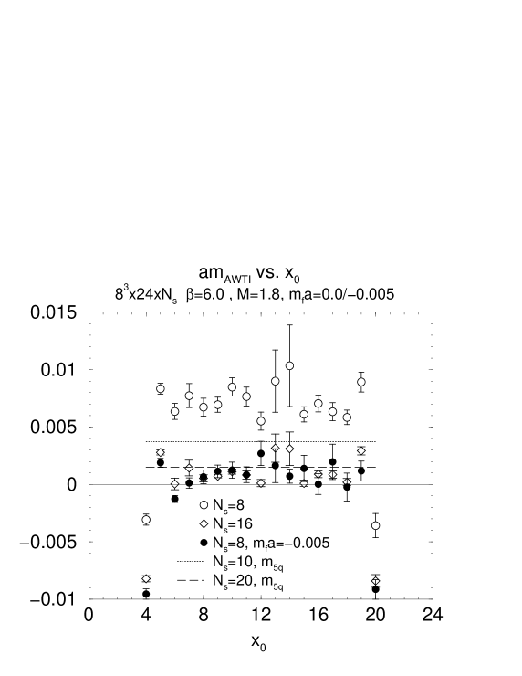
Figure 2: $am_{\rm AWTI}$ as a function of $x_{0}$ at $\beta\!=\!6.0$ on an $8^{3}\!\times\!24\!\times\!N_{s}$ lattice at $m_{f}a=0$ with $N_{s}=8$(open circles) and 16(open diamonds) and at $m_{f}=-0.005$ with $N_{s}=8$(solid circles), together with $m_{5q}$ at $N_{s}=10$(dotted line) and $N_{s}=20$ (dashed line)chiral .

In Fig. 2, $am_{\rm AWTI}$ in the quenched DWQCD with our boundary condition is plotted as a function of $x_{0}$ on $8^{3}\times 24\times N_{s}$ lattices with $m_{f}a=0$ and $M=1.8$ at $\beta=6.0$ for the plaquette gauge action. Since the $x_{0}$ dependence is weak away from the boundaries, we non-perturbatively confirm the conclusion in the free case that the effect of the Dirichlet boundary condition is negligible. Interestingly $m_{\rm AWTI}$ is non-zero even at $m_{f}a=0$, and becomes smaller for larger $N_{s}$. Moreover the value is consistent with $m_{5q}$, a measure of the explicit chiral symmetry breaking calculated from the conserved axial-vector current of DWQCDchiral . This fact suggests $m_{\rm AWTI}$ in our finite volume scheme may be a better alternative as the measure of explicit chiral symmetry breaking in DWQCD, since it can be calculated directly at $m_{f}a=0$ with much less computational cost. Note also that the large explicit breaking in $m_{\rm AWTI}$ at $N_{s}=8$ (open circles) is compensated if one takes a negative quark mass of $m_{f}=-0.005$ (filled circles). This demonstrates that the domain-wall fermion at $N_{s}\not=\infty$ can be considered as a highly improved Wilson fermionvpp .

IV.2 Renormalization factors

The non-perturbative renormalization factors for vector and axial-vector currents are defined by $Z_{V}(1+b_{V}m_{f}a)=f_{1}/f_{V}(x_{0})$ and $Z_{A}^{2}=2f_{1}/f_{AA}(x_{0},x_{0}^{+},x_{0}^{-})$, where we fix $x_{0}^{\pm}=T/2\pm T/4$ and put $m_{f}a=0$ for $Z_{A}$. In Fig. 3, $Z_{V}$ and $Z_{A}$ are plotted as a function of $x_{0}$ on $8^{3}\times 16\times 16$ at $\beta=6.0$ with $M=1.8$ and $m_{f}=0$. Similar to the case of $am_{\rm AWTI}$ a plateau is seen away from the boundaries. The relation $Z_{V}=Z_{A}$, valid exactly in perturbation theory, is satisfied non-perturbatively within 1–2%. Moreover the magnitude of $Z_{V,A}$ almost agrees with the mean-field(MF) improved one-loop value. We also observe that $Z_{V}$ is insensitive to boundary parameters such as the 2-loop boundary counter-terms for gauge fields and the parameter $\theta$ of the twisted boundary condition for quarks.

IV.3 Dependence of $Z_{V,A}$ on $M$

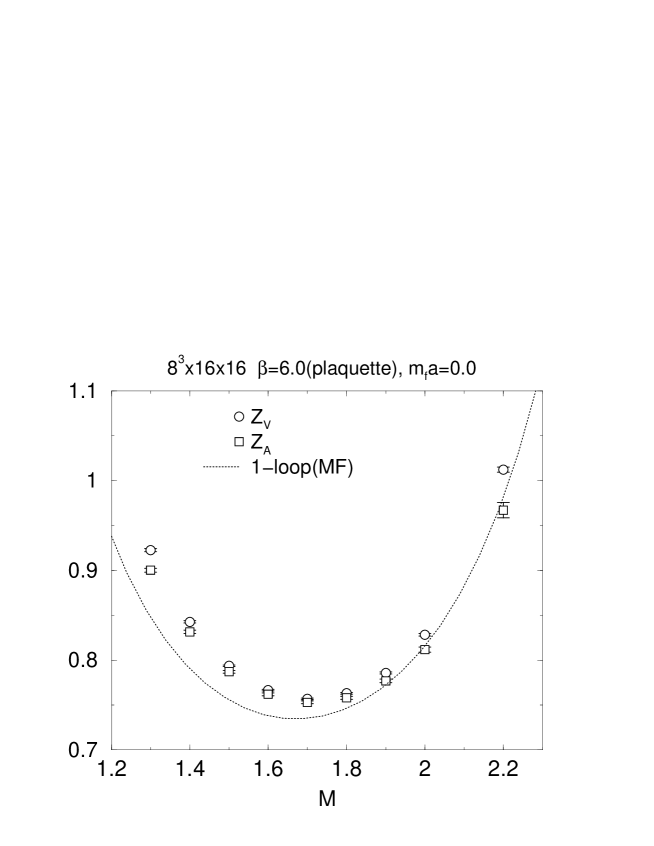
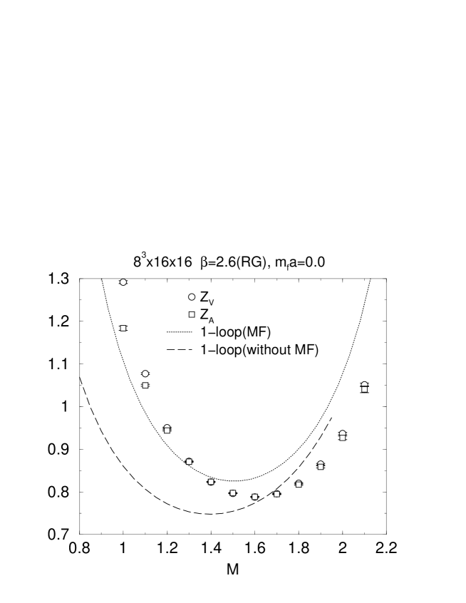
Figure 4: $Z_{V}$ and $Z_{A}$ vs $M$ on $8^{3}\times 16\times 16$ at $\beta=6.0$ for plaquette action(upper) and at $\beta=2.6$ for the RG action(lower). Perturbative estimates are given at 1-loop with the MF improvement (solid lines) and without it (dashed line).

We calculate $Z_{V}$ and $Z_{A}$ in the quenched DWQCD at $a^{-1}\simeq 2$ GeV with the plaquette action ($\beta=6.0$) and with the renormalization group(RG) improved action ($\beta=2.6$) on an $8^{3}\times 16\times 16$ lattice with $m_{f}a=0$ for $M=1.0\sim 2.2$. The results are summarized in Fig. 4, where $Z_{V}$ and $Z_{A}$ are plotted as a function of $M$, together with one-loop perturbative estimates with and without mean-field (MF) improvementAIKT . For both gauge actions, $Z_{V}\simeq Z_{A}$ holds, and they have a minimum at $M\simeq 1.7$ for the plaquette action or $M\simeq 1.6$ for the RG action. The deviation from $Z_{V}=Z_{A}$ becomes larger as $M$ goes far away from the minimum. This suggests that the chiral symmetry breaking effect is proportional to $|M-M_{\rm min.}|^{N_{s}}$. Perturbative estimates without MF improvement fail, particularly for the plaquette action for which the curve can not be placed in the figure. The MF improvement makes the agreement much better for both actions.

V Results

We extract $Z_{V}$ and $Z_{A}$ at various values of $g^{2}$ for both plaquette and RG improved gauge actions on a $N_{l}^{3}\times N_{t}\times N_{s}=8^{3}\times 16\times 16$ lattice. In addition we employ a different 4 dimensional lattice size, $N_{l}^{3}\times N_{t}=12^{3}\times 24$ or $4^{3}\times 8$, while keeping $N_{s}=16$, in order to investigate $a/L=1/N_{l}$ dependences of $Z_{V}$ and $Z_{A}$. Simulation parameters are given in Table LABEL:tab:param, together with the lattice spacing $a$, obtained from the global parametrization for the string tension as a function of $g^{2}$:

$$\sigma^{1/2}a = a(g^{2})\frac{1+c_{2}\hat{a}^{2}(g^{2})+c_{4}\hat{a}^{4}(g^{2})+c_{6}\hat{a}^{6}(g^{2})}{c_{0}}$$ (20)

$$a(g^{2}) = (b_{0}g^{2})^{-b_{1}}\exp[-\frac{1}{2b_{0}g^{2}}]$$ (21)

$$\hat{a}(g^{2}) = \frac{a(g^{2})}{a(g_{0}^{2})}$$ (22)

where $b_{0}=11/(4\pi)^{2}$, $b_{1}=102/(4\pi)^{4}$ (the coefficients of $\beta$ function in the quenched theory). The coefficients of the parametrization become $c_{0}=0.01364$, $c_{2}=0.2731$, $c_{4}=-0.01545$ and $c_{6}=0.01975$ with $g_{0}^{2}=1.0$ for the plaquette actionsigmaP , and $c_{0}=0.524$, $c_{2}=0.274$, $c_{4}=0.105$ and $c_{6}=0$ with $g_{0}^{2}=6/2.4$ for the RG actionsigmaRG . We use $\sigma^{1/2}$ = 0.44 GeV to get $a$ in the Table LABEL:tab:param. Gauge fields are updated by the pseudo-heat bath algorithm with five hits, followed by four over-relaxation sweeps; the combination of these updates is called an iteration. After 2000 iterations for a thermalization, we calculate the fermionic correlation functions on the gauge configurations separated by 200 iterations. On each $M$ at given $\beta$, different gauge configurations are used to evaluate $Z_{V}$ and $Z_{A}$, so that the measurements of $Z$’s at different $M$ are independent. Raw data of $Z_{V}$(the 3rd and 4th columns) and $Z_{A}$(the 2nd column) are compiled in Table LABEL:tab:resultP for the plaquette action and Table LABEL:tab:resultRG for the RG action.

It has been shown that $Z_{V}=Z_{A}$ in perturbation theory for DWQCDAIKT , and, as already mentioned in the previous section, this equality is well satisfied non-perturbatively at $\beta=6.0$ for the plaquette action and at $\beta=2.6$ for the RG action. Although the violation of this equality becomes larger at stronger coupling(at $\beta=5.8$ for the plaquette action and at $\beta=2.4,2.2$ for the RG action), or at the values of $M$ far away from the ”minimum” where the chiral symmetry is best realized, we define $Z_{A}=Z_{V}$ for DWQCD in this paper, taking numerical values of $Z_{V}$ as the renormalization factor for both vector and axial-vector currents. Therefore we discuss $Z_{V}$ only hereafter.

V.1 $Z_{V}$ as a function of $M$

At each $g^{2}$, we fit $Z_{V}$ as a function of $M$ by the formula

$$Z_{V}^{\rm fit} = \frac{B_{0}+B_{1}(M-M_{c})+B_{2}(M-M_{c})^{2}}{1+A_{2}(M-M_{c})^{2}},$$ (23)

which is suggested by the perturbation theoryAIKT . Results for fit parameters $M_{C}$, $A_{2}$ and $B_{i}$($i=0,1,2$) are given in Tables 4 and 5, together with $\delta^{\rm max}$, the maximum of the relative errors $\delta$ defined by

$$\delta = (Z_{V}-Z_{V}^{\rm fit})/Z_{V}.$$ (24)

As we observe that $\delta^{\rm max}$ are typically less than 1% and at most a few %, the fit describes data well.

V.2 Finite $a/L$ errors

Errors of $Z_{V}$ associated with the lattice spacing are $O((a/L)^{2}$ in the $N_{s}\rightarrow\infty$ limit, or $O(e^{-\alpha N_{s}}\times a/L)$ at finite $N_{s}$. If $a/L=1/N_{l}=1/8$ is kept fixed at all value of $g^{2}$, the scaling violation in $Z_{V,A}$ remains even in the $g^{2}\rightarrow 0$ limit. In order to reduce or remove this scaling violation, we interpolate or extrapolate $Z_{V}$ to the fixed value of $L$ at each $g^{2}$, using data on two different spatial lattice sizes $L$. For the interpolation or the extrapolation, we adopt the linear dependence:

$$Z_{V}(a/L) = Z_{V}+c\frac{a}{L}=Z_{V}+c\frac{1}{N_{l}}.$$ (25)

Since only data at two different $N_{l}$ are available, the value of $Z_{V}$ at fixed $L$ and its error are estimated by

$$Z_{V}(a/L) = \frac{Z_{V}^{2}x_{1}-Z_{V}^{1}x_{2}}{x_{12}}$$ (26)

$$\delta Z_{V}(a/L) = \frac{|\delta Z_{V}^{2}x_{1}|+|\delta Z_{V}^{1}x_{2}|}{x_{12}}$$ (27)

where $Z_{V}^{i}=Z_{V}(1/N_{i})$, $x_{i}=1/N_{i}-a/L$ ($i=1,2$) and $x_{12}=1/N_{1}-1/N_{2}$ with $N_{1}=8$ and $N_{2}=4$ or 12, and $\delta$ means the error of the corresponding quantity. To estimate the systematic uncertainty associated with the assumption eq. (25), we alternatively employ the quadratic form:

$$Z_{V}(a/L) = Z_{V}+c\frac{a^{2}}{L^{2}}=Z_{V}+c\frac{1}{N_{l}^{2}},$$ (28)

and calculate $Z_{V}(1/L)$. A difference in $Z_{V}(a/L)$ between the linear and the quadratic dependences is quadratically added to $\delta Z_{V}(a/L)$ as an estimate of the systematic uncertainty, while the central value of $Z_{V}(a/L)$ is taken from the value obtained from the linear assumption.

In Tables LABEL:tab:resultP and LABEL:tab:resultRG, the values of $Z_{V}(a/L)$ are given at $L=L^{*}=8a(\beta=6.0)$ (the 5th column), where $a(\beta=6.0)$ is the lattice spacing at $\beta=6.0$ for the plaquette action, and at $L=\infty$ (the 8th column). While the former definition of $Z_{V}$ contains an $O(a/L^{*})$ error, which vanishes in the continuum limit, the latter one is free from such an uncertainty. By taking the difference of $Z_{V}$ between $L=L^{*}$ and $\infty$, the $a/L^{*}$ error in $Z_{V}$ is estimated to be 0.06 at $M=1.8$ and $\beta=6.0$ ($a^{-1}=$2 GeV) for the plaquette action, or 0.02 at $M=1.7$ and $\beta=2.6$ ($a^{-1}=$1.9 GeV) for the RG action. On the other hand, the error associated with the extrapolation in $L$ is larger at $L=\infty$: 0.002 ($L=L^{*}$) and 0.025 ($L=\infty$) at the previous parameters for the plaquette action, and 0.002 and 0.017 for the RG action. Moreover $Z_{V}$ at $L=\infty$ monotonically decreases as $M$ increases at $a^{-1}<2$ GeV, while it has the minimum in $M$ at $a^{-1}\geq 2$ GeV. Only the latter behaviour is observed for $Z_{V}$ at $L=L^{*}$. We suspect that the behaviour of $Z_{V}$ at $L=\infty$ is related to the existence of (near) zero eigenvalues for the hermitian Wilson-Dirac operator at $a^{-1}<2$: It suggests that the gap of zero eigenvalues for the the hermitian Wilson-Dirac operator is closed at $a^{-1}<2$ for both plaquette and RG actions. This speculation is consistent with the observation that DWQCD can not realize an exact chiral symmetry even in the $N_{s}\rightarrow\infty$ limit at $a^{-1}\simeq$ 1 GeV for both gauge actionschiral , though the quenched artifact may explain the observationGS .

V.3 $Z_{V}$ as a function of $M$ and $g^{2}$

For the latter uses, we parametrize $Z_{V}$ as a function of $M$ and $g^{2}$, in order to obtain $Z$ at arbitrary (interpolated) values of $\beta$ and $M$. We adopt the following fitting function suggested by the perturbation theoryAIKT :

$$Z_{V}(g^{2},M) = \frac{B_{0}(g^{2})+B_{1}(g^{2})(M-M_{c}(g^{2}))+B_{2}(g^{2})(M-M_{c}(g^{2}))^{2}}{1+A_{2}(g^{2})(M-M_{c}(g^{2}))^{2}}$$ (29)

$$M_{c}(g_{2}) = \displaystyle\frac{1+(c_{M}+a_{1})g^{2}+a_{2}g^{4}+a_{3}g^{6}}{1+a_{1}g^{2}}$$

$$B_{0}(g_{2}) = \displaystyle\frac{1+(c_{0}+a_{4})g^{2}+a_{5}g^{4}+a_{6}g^{6}}{1+a_{4}g^{2}}$$

$$A_{2}(g_{2}) = -\displaystyle\frac{1+(d_{2}+a_{7})g^{2}+a_{9}g^{4}+a_{10}g^{6}}{1+a_{7}g^{2}+a_{8}g^{4}}$$

$$B_{1}(g_{2}) = c_{1}g^{2}$$

$$B_{2}(g_{2}) = \displaystyle\frac{c_{2}g^{2}}{1+a_{11}g^{2}}$$

where $c_{M}$, $d_{2}$ and $c_{i}$($i=0,1,2$) are values of 1-loop coefficients for $M_{c}$, $A_{2}$ and $B_{i}$($i=0,1,2$)AIKT , which are given by

$$(c_{M},d_{2},c_{0},c_{1},c_{2}) = (0.4177,0.01173,-0.1456,2.311\times 10^{-3},-5.172\times 10^{-3})$$

for the plaquette action and

$$(c_{M},d_{2},c_{0},c_{1},c_{2}) = (0.2070,8.131\times 10^{-3},-0.07449,1.912\times 10^{-3},-4.154\times 10^{-3})$$

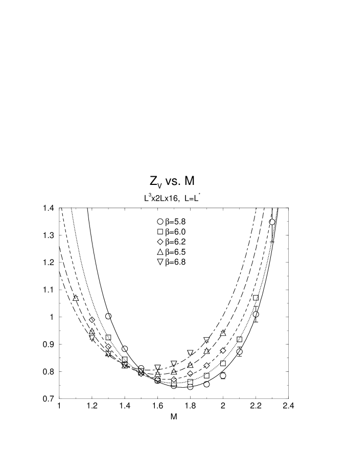
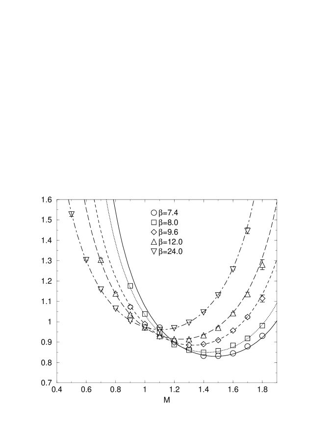
Figure 5: $Z_{V}$ as a function $M$ on $L^{3}\times 2L\times 16$ with $L=L^{*}$ at several values of $\beta$ for the plaquette action.

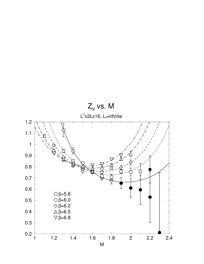
Figure 6: $Z_{V}$ as a function $M$ on $L^{3}\times 2L\times 16$ with $L=\infty$ at several values of $\beta$ for the plaquette action. Solids symbols are excluded for the fits.

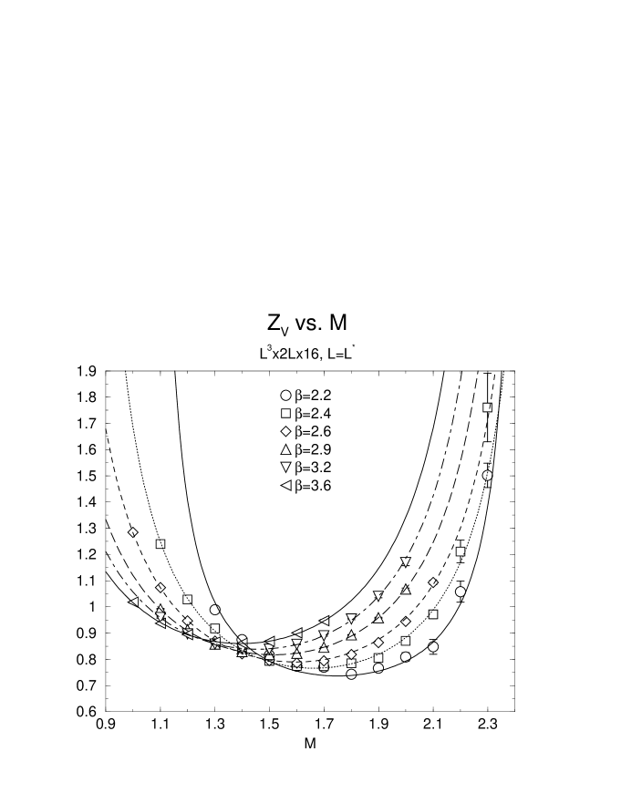
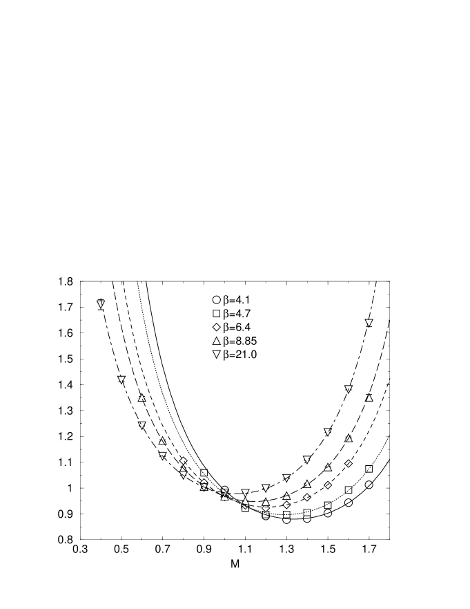
Figure 7: $Z_{V}$ as a function $M$ on $L^{3}\times 2L\times 16$ with $L=L^{*}$ at several values of $\beta$ for the RG action.

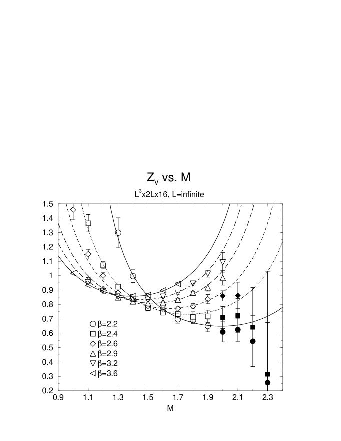
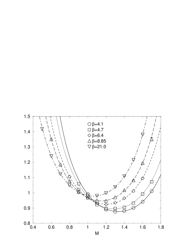
Figure 8: $Z_{V}$ as a function $M$ on $L^{3}\times 2L\times 16$ with $L=\infty$ at several values of $\beta$ for the RG action. Solids symbols are excluded for the fits.

for the RG action. These constraints make $M_{c}$, $A_{2}$ and $B_{i}$($i=0,1,2$) consistent with the perturbation theory at 1-loop. Numerical values of parameters $a_{i}$ ($i=1\sim 11$) are given in Table 6 for both $L=L^{*}$ and $L=\infty$. In order to show the quality of the fits, we plot the fitting curves for $Z_{V}(a/L^{*})$ and $Z_{V}(0)$ in Fig.5 and Fig.6 for the plaquette action, and in Fig.7 and Fig.8 for the RG action, respectively. Furthermore, we compile $Z_{V}(g^{2},M)$ and the relative deviation

$$\delta_{G} = \displaystyle\frac{Z_{V}-Z_{V}(g^{2},M)}{Z_{V}}$$ (30)

in the 6th and 7th columns or the 9th and 10th columns of Tables LABEL:tab:resultP and LABEL:tab:resultRG, where $Z_{V}=Z_{V}(a/L^{*})$ or $Z_{V}(0)$, respectively. In the fit for $Z_{V}(0)$ we exclude a few points for larger values of $M$ at $\beta=5.8$ and $6.0$ for the plaquette action and at $\beta=2.2,2.4,2.6$ for the RG action, which are represented by solid symbols in the figures and are marked by ”- ” in the tables. These data for $Z_{V}(0)$ have large errors and large values of $\delta_{G}$. From the figures and tables we observe that the fits works well and $\delta_{G}$ are less than a few %, except a few points at the edges of the range in $M$ employed for the simulations.

VI Conclusions and Discussions

We calculate the renormalization factors for the vector and axial-vector currents in the quenched DWQCD for both plaquette and RG actions. After several tests are performed at $a^{-1}\simeq$ 2 GeV, we obtain $Z_{V}$, which is assumed to be equal to $Z_{A}$, at $L=\infty$ as well as $L=L^{*}$ for the wide ranges of $g^{2}$ and $M$. We globally fit $Z_{V}$ as a function of $g^{2}$ and $M$.

We now propose how to use these results for the future simulations of the quenched DWQCD.

1. For the DWQCD to realize the chiral symmetry well, one should take at least $a^{-1}\geq$ 2 GeV. This condition is satisfied at $\beta\geq 6.0$ for the plaquette action or at $\beta\geq 2.6$ for the RG action.

2. One should choose the optimal value of $M$, which minimizes the violation of the chiral symmetry at finite $N_{s}$. A good candidate is the choice that $M\simeq M_{c}(g^{2})$, where

   $$M_{c}(g^{2}) = \frac{1+(c_{M}+a_{1})g^{2}+a_{2}g^{4}+a_{3}g^{6}}{1+a_{1}g^{2}}.$$ (31)

   The parameters $a_{1,2,3}$ are given in Table 6.

3. If the simulation point at $g^{2}$ and $M$ can be found in the Table LABEL:tab:resultP or Table LABEL:tab:resultRG, one should use $Z_{V}$ in the table as the renormalization factor for the vector or axial-vector current. To remove $O(a/L)$ errors in $Z_{V}$, it is better to take $Z_{V}$ at $L=\infty$, though the statistical error of $Z_{V}$ is larger in this case. One may use $Z_{V}$ at $L=L^{*}$ to estimate the size of $O(a/L)$ errors in $Z_{V}$.

4. If $g^{2}$ or $M$ for the simulation point is not found in the tables, one should use the fitting function given in eq. (29) with the parameters in Table 6. The error of $Z_{V}$ is estimated from the errors of $Z_{V}$ at the nearest points in $g^{2}$ and $M$, which can be found in the tables.

We are encouraged with the present results to proceed to an extension of the present work to scale-dependent cases such as quark masses and four-quark operators needed for $B_{K}$, implementing the SF boundary condition for the domain-wall fermionsAKT .

Table 1: Simulation parameters

Plaquette				RG improved
$\beta$	$a^{-1}$(GeV)	# of conf.	# of conf.	$\beta$	$a^{-1}$(GeV)	# of conf.	# of conf.
		$8^{3}\times 16\times 16$	$4^{3}\times 8\times 16$			$8^{3}\times 16\times 16$	$4^{3}\times 8\times 16$
				2.2	1.0	100	100-200
5.8	1.4	100	100	2.4	1.4	100	100-200
		$8^{3}\times 16\times 16$	$12^{3}\times 24\times 16$			$8^{3}\times 16\times 16$	$12^{3}\times 24\times 16$
6.0	2.0	100	20	2.6	1.9	100	30
6.2	2.7	100	10-30	2.9	2.9	100	15-50
6.5	4.1	100	15-25	3.2	4.3	100	20-25
6.8	6.1	100	10-15	3.6	6.8	100	20-25
7.4	12	100	10-20	4.1	12	100	20-25
8.0	25	40	7-15	4.7	23	40	10-20
9.6	156	40	10	6.4	154	40	10-20
12.0	2502	20	10	8.85	2523	20	10-15
24.0	3.2$\times 10^{9}$	20	10	21.0	3.6$\times 10^{9}$	20	10

Table 2: Results for the plaquette action.

	$Z_{A}$	$Z_{V}$		$Z_{V}$ at $L=L^{*}$			$Z_{V}$ at $L=\infty$
$M$	$8^{3}\times 16$	$8^{3}\times 16$	$4^{3}\times 8$	$Z_{V}^{L}$	Fit	$\delta_{G}$(%)	$Z_{V}^{L}$	Fit	$\delta_{G}$(%)
$\beta=5.8$, $a^{-1}$=1.4 GeV, $L^{*}/a=5.6$
1.3	0.7724(119)	1.0398(69)	0.9535(78)	1.0028(87)	1.0153	1.2	1.1260(596)	1.1318	0.5
1.4	0.7203(94)	0.9013(37)	0.8603(64)	0.8837(48)	0.8815	0.2	0.9423(290)	0.9406	0.2
1.5	0.6914(104)	0.8179(28)	0.7852(63)	0.8122(33)	0.8062	0.7	0.8313(123)	0.8250	0.8
1.6	0.6603(83)	0.7624(41)	0.7731(90)	0.7670(46)	0.7641	0.4	0.7516(141)	0.7514	0.02
1.7	0.6383(98)	0.7348(30)	0.7659(68)	0.7481(42)	0.7449	0.4	0.7036(226)	0.7046	0.1
1.8	0.6377(82)	0.7245(30)	0.7711(41)	0.7444(45)	0.7443	0.01	0.6778(319)	0.6768	0.1
1.9	0.6309(79)	0.7238(42)	0.7939(134)	0.7538(85)	0.7624	1.1	0.6537(493)	0.6641	1.6
2.0	0.6290(84)	0.7330(55)	0.8550(129)	0.7853(118)	0.8029	2.2	0.6110(831)	-	-
2.1	0.6710(115)	0.7894(54)	0.9848(122)	0.8732(171)	0.8755	0.3	0.5940(1313)	-	-
2.2	0.6722(149)	0.8660(81)	1.2024(160)	1.0102(287)	1.0037	0.6	0.5296(2254)	-	-
2.3	0.7080(203)	1.0079(106)	1.8025(796)	1.3484(736)	1.2499	7.3	0.2132(5361)	-	-
$\beta=6.0$, $a^{-1}$=2.0 GeV, $L^{*}/a=8.0$
1.3	0.9002(21)	0.9252(30)	0.9308(36)	0.9252(30)	0.9253	0.01	0.9421(141)	0.9438	0.2
1.4	0.8330(21)	0.8446(25)	0.8472(32)	0.8446(25)	0.8431	0.2	0.8526(112)	0.8491	0.4
1.5	0.7884(20)	0.7950(22)	0.7927(44)	0.7950(22)	0.7935	0.2	0.7656(227)	0.7885	3.0
1.6	0.7633(19)	0.7674(21)	0.7635(50)	0.7674(21)	0.7666	0.1	0.7555(163)	0.7511	0.6
1.7	0.7541(19)	0.7572(21)	0.7438(42)	0.7572(21)	0.7578	0.1	0.7169(208)	0.7316	2.0
1.8	0.7589(20)	0.7628(21)	0.7439(35)	0.7628(21)	0.7659	0.4	0.7062(254)	0.7272	3.0
1.9	0.7781(23)	0.7852(21)	0.7761(43)	0.7852(21)	0.7921	0.9	0.7577(175)	0.7375	3.0
2.0	0.8153(30)	0.8300(25)	0.8044(58)	0.8300(25)	0.8406	1.3	0.7532(356)	0.7636	1.4
2.1	0.8802(52)	0.9179(34)	0.8647(84)	0.9179(34)	0.9210	0.3	0.7583(690)	0.8092	6.7
2.2	0.9941(95)	1.0706(48)	0.9722(81)	1.0706(48)	1.0535	1.6	0.7754(1209)	-	-
$\beta=6.2$, $a^{-1}$=2.7 GeV, $L^{*}/a=10.8$
1.2	0.9734(15)	0.9896(21)	0.9899(25)	0.9898(20)	0.9926	0.3	0.9904(87)	0.9982	0.8
1.3	0.8858(11)	0.8937(14)	0.8911(19)	0.8917(15)	0.8921	0.04	0.8859(70)	0.8947	1.0
1.4	0.8294(07)	0.8321(13)	0.8242(18)	0.8260(15)	0.8295	0.4	0.8084(113)	0.8284	2.5
1.5	0.7957(10)	0.7969(16)	0.7915(32)	0.7927(25)	0.7923	0.1	0.7805(121)	0.7872	0.9
1.6	0.7764(09)	0.7781(13)	0.7700(27)	0.7718(21)	0.7744	0.3	0.7537(129)	0.7651	1.5
1.7	0.7766(10)	0.7778(14)	0.7693(28)	0.7712(23)	0.7731	0.2	0.7524(135)	0.7589	0.9
1.8	0.7892(11)	0.7949(18)	0.7918(21)	0.7925(17)	0.7884	0.5	0.7855(82)	0.7681	2.2
1.9	0.8196(14)	0.8319(19)	0.8190(23)	0.8219(19)	0.8223	0.05	0.7932(174)	0.7936	0.05
2.0	0.8659(27)	0.8908(22)	0.8734(30)	0.8772(24)	0.8802	0.3	0.8386(231)	0.8389	0.04
$\beta=6.5$, $a^{-1}$=4.1 GeV, $L^{*}/a=16.4$
1.1	1.0458(13)	1.0656(18)	1.0689(26)	1.0707(42)	1.0635	0.7	1.0757(95)	1.0588	1.6
1.2	0.9416(10)	0.9469(16)	0.9480(19)	0.9485(31)	0.9449	0.4	0.9500(67)	0.9431	0.7
1.3	0.8715(08)	0.8728(13)	0.8698(16)	0.8682(26)	0.8700	0.2	0.8638(65)	0.8690	0.6
1.4	0.8285(08)	0.8290(12)	0.8256(16)	0.8238(27)	0.8236	0.02	0.8188(68)	0.8226	0.5
1.5	0.8042(06)	0.8042(11)	0.8024(11)	0.8014(19)	0.7981	0.4	0.7987(47)	0.7966	0.3
1.6	0.7963(07)	0.7976(08)	0.7939(23)	0.7919(36)	0.7898	0.3	0.7864(84)	0.7876	0.2
1.7	0.8051(07)	0.8082(12)	0.8031(14)	0.8004(23)	0.7976	0.3	0.7930(77)	0.7945	0.2
1.8	0.8246(10)	0.8335(14)	0.8279(23)	0.8249(38)	0.8226	0.3	0.8167(101)	0.8181	0.2
1.9	0.8687(17)	0.8853(17)	0.8797(26)	0.8767(41)	0.8682	1.0	0.8685(108)	0.8615	0.8
2.0	0.9345(29)	0.9730(21)	0.9531(25)	0.9424(52)	0.9419	0.1	0.9132(254)	0.9311	2.0
$\beta=6.8$, $a^{-1}$=6.1 GeV, $L^{*}/a=24.4$
1.2	0.9250(07)	0.9250(13)	0.9233(13)	0.9215(31)	0.9211	0.03	0.9198(52)	0.9192	0.1
1.3	0.8667(07)	0.8656(12)	0.8647(19)	0.8638(41)	0.8610	0.3	0.8629(64)	0.8605	0.3
1.4	0.8317(06)	0.8304(10)	0.8269(20)	0.8232(43)	0.8250	0.2	0.8197(75)	0.8253	0.7
1.5	0.8156(06)	0.8157(09)	0.8085(19)	0.8011(49)	0.8078	0.8	0.7940(105)	0.8088	1.9
1.6	0.8140(07)	0.8147(12)	0.8141(14)	0.8134(31)	0.8070	0.8	0.8129(49)	0.8088	0.5
1.7	0.8300(07)	0.8359(10)	0.8319(11)	0.8279(30)	0.8227	0.6	0.8239(63)	0.8253	0.2
1.8	0.8575(11)	0.8692(14)	0.8685(13)	0.8677(31)	0.8568	1.3	0.8670(50)	0.8603	0.8
1.9	0.9116(19)	0.9393(16)	0.9271(17)	0.9147(63)	0.9142	0.1	0.9027(158)	0.9189	1.8
$\beta=7.4$, $a^{-1}$=12 GeV, $L^{*}/a=48$
1.1	0.9761(06)	0.9762(11)	0.9744(14)	0.9717(41)	0.9693	0.2	0.9708(53)	0.9677	0.3
1.2	0.9090(07)	0.9078(09)	0.9054(12)	0.9019(37)	0.9005	0.2	0.9007(48)	0.9002	0.1
1.3	0.8646(05)	0.8631(08)	0.8642(14)	0.8658(37)	0.8582	0.9	0.8663(45)	0.8588	0.9
1.4	0.8437(05)	0.8441(08)	0.8398(16)	0.8335(53)	0.8359	0.3	0.8313(72)	0.8376	0.8
1.5	0.8394(05)	0.8403(08)	0.8374(13)	0.8332(41)	0.8309	0.3	0.8318(54)	0.8337	0.2
1.6	0.8497(05)	0.8535(08)	0.8504(23)	0.8457(63)	0.8424	0.4	0.8442(80)	0.8467	0.3
1.7	0.8748(07)	0.8854(09)	0.8829(20)	0.8792(55)	0.8718	0.8	0.8780(69)	0.8782	0.02
1.8	0.9150(14)	0.9418(11)	0.9375(10)	0.9311(43)	0.9232	0.8	0.9289(63)	0.9325	0.4
$\beta=8.0$, $a^{-1}$=25 GeV, $L^{*}/a=100$
0.9	1.1644(16)	1.1842(22)	1.1814(20)	1.1764(73)	1.1674	0.8	1.1757(82)	1.1669	0.8
1.0	1.0421(08)	1.0437(13)	1.0431(14)	1.0383(49)	1.0340	0.4	1.0378(55)	1.0337	0.4
1.1	0.9578(08)	0.9575(12)	0.9538(10)	0.9471(51)	0.9486	0.2	0.9462(60)	0.9485	0.2
1.2	0.9031(07)	0.9024(09)	0.8972(17)	0.8881(71)	0.8946	0.7	0.8868(83)	0.8948	0.9
1.3	0.8715(05)	0.8712(10)	0.8674(11)	0.8607(51)	0.8634	0.3	0.8598(60)	0.8640	0.5
1.4	0.8576(06)	0.8565(09)	0.8542(09)	0.8501(37)	0.8506	0.1	0.8495(43)	0.8520	0.3
1.5	0.8601(06)	0.8615(11)	0.8600(07)	0.8575(32)	0.8548	0.3	0.8572(36)	0.8572	0.0
1.6	0.8790(08)	0.8846(14)	0.8846(11)	0.8847(40)	0.8763	0.9	0.8847(44)	0.8802	0.5
1.7	0.9164(11)	0.9341(10)	0.9284(19)	0.9186(78)	0.9180	0.1	0.9172(91)	0.9241	0.8
1.8	0.9738(21)	1.0074(18)	0.9979(14)	0.9812(105)	0.9860	0.5	0.9789(127)	0.9953	1.7
$\beta=9.6$, $a^{-1}$=156 GeV, $L^{*}/a=624$
0.9	1.0897(07)	1.0921(11)	1.0855(08)	1.0726(83)	1.0787	0.6	1.0723(86)	1.0817	0.9
1.0	0.9994(06)	0.9973(09)	0.9947(09)	0.9897(43)	0.9892	0.1	0.9896(44)	0.9901	0.1
1.1	0.9412(05)	0.9395(07)	0.9356(07)	0.9279(52)	0.9324	0.5	0.9278(54)	0.9322	0.5
1.2	0.9053(05)	0.9032(09)	0.9016(05)	0.8984(30)	0.8995	0.1	0.8983(31)	0.8986	0.03
1.3	0.8895(05)	0.8884(07)	0.8876(06)	0.8859(25)	0.8858	0.01	0.8859(25)	0.8847	0.1
1.4	0.8928(06)	0.8938(10)	0.8926(11)	0.8903(40)	0.8899	0.05	0.8903(41)	0.8887	0.2
1.5	0.9129(04)	0.9181(07)	0.9154(08)	0.9099(41)	0.9120	0.2	0.9098(42)	0.9112	0.2
1.6	0.9471(08)	0.9621(09)	0.9605(12)	0.9573(44)	0.9551	0.2	0.9572(44)	0.9550	0.2
1.7	1.0023(17)	1.0362(12)	1.0319(10)	1.0236(63)	1.0253	0.2	1.0235(64)	1.0266	0.3
1.8	1.0946(32)	1.1568(17)	1.1425(18)	1.1145(178)	1.1346	1.8	1.1139(183)	1.1383	2.2
$\beta=12.0$, $a^{-1}$=2502 GeV, $L^{*}/a=10008$
0.7	1.2733(14)	1.3174(18)	1.3131(14)	1.3043(76)	1.2946	0.7	1.3043(76)	1.3051	0.1
0.8	1.1437(07)	1.1500(12)	1.1461(09)	1.1383(59)	1.1370	0.1	1.1383(60)	1.1418	0.3
0.9	1.0467(06)	1.0440(10)	1.0411(06)	1.0356(44)	1.0364	0.1	1.0355(44)	1.0381	0.2
1.0	0.9803(06)	0.9759(10)	0.9747(04)	0.9724(26)	0.9723	0.01	0.9724(26)	0.9720	0.04
1.1	0.9405(04)	0.9369(06)	0.9346(09)	0.9301(39)	0.9341	0.4	0.9301(39)	0.9326	0.3
1.2	0.9200(03)	0.9179(05)	0.9170(05)	0.9151(22)	0.9166	0.2	0.9151(22)	0.9142	0.1
1.3	0.9202(06)	0.9199(07)	0.9181(05)	0.9145(31)	0.9175	0.3	0.9145(31)	0.9145	0.0
1.4	0.9360(05)	0.9391(07)	0.9372(03)	0.9332(29)	0.9370	0.4	0.9332(29)	0.9336	0.04
1.5	0.9685(06)	0.9806(09)	0.9772(08)	0.9705(50)	0.9776	0.7	0.9705(50)	0.9738	0.3
1.6	1.0200(14)	1.0473(14)	1.0456(03)	1.0423(39)	1.0448	0.2	1.0423(39)	1.0408	0.1
1.7	1.1011(30)	1.1572(12)	1.1501(08)	1.1360(91)	1.1500	1.2	1.1359(92)	1.1460	0.9
1.8	1.2299(54)	1.3400(20)	1.3202(15)	1.2805(245)	1.3150	2.7	1.2805(246)	1.3114	2.4
$\beta=24.0$, $a^{-1}=3.2\times 10^{9}$ GeV, $L^{*}/a=1.28\times 10^{10}$
0.5	1.4168(27)	1.5526(11)	1.5441(05)	1.5272(106)	1.5323	0.3	1.5272(106)	1.5406	0.9
0.6	1.2735(09)	1.3079(07)	1.3063(04)	1.3030(27)	1.3003	0.2	1.3030(27)	1.3043	0.1
0.7	1.1603(02)	1.1604(05)	1.1597(06)	1.1583(21)	1.1565	0.2	1.1583(21)	1.1582	0.01
0.8	1.0746(03)	1.0669(04)	1.0662(03)	1.0647(14)	1.0644	0.03	1.0647(14)	1.0647	0.0
0.9	1.0154(03)	1.0083(05)	1.0069(04)	1.0040(22)	1.0064	0.2	1.0040(22)	1.0059	0.2
1.0	0.9802(03)	0.9752(04)	0.9738(03)	0.9710(20)	0.9738	0.3	0.9710(20)	0.9725	0.2
1.1	0.9666(02)	0.9629(03)	0.9619(02)	0.9600(15)	0.9619	0.2	0.9600(15)	0.9602	0.02
1.2	0.9716(02)	0.9696(03)	0.9693(02)	0.9685(09)	0.9695	0.1	0.9685(09)	0.9673	0.1
1.3	0.9946(03)	0.9976(04)	0.9969(02)	0.9956(13)	0.9974	0.2	0.9956(13)	0.9947	0.1
1.4	1.0350(03)	1.0493(06)	1.0485(02)	1.0468(17)	1.0492	0.2	1.0468(17)	1.0461	0.1
1.5	1.0959(08)	1.1324(06)	1.1316(04)	1.1300(19)	1.1328	0.2	1.1300(19)	1.1290	0.1
1.6	1.1820(23)	1.2638(06)	1.2615(04)	1.2571(32)	1.2630	0.5	1.2571(32)	1.2584	0.1
1.7	1.3151(40)	1.4815(07)	1.4698(08)	1.4464(143)	1.4706	1.7	1.4464(143)	1.4647	1.3

Table 3: Results for the RG action.

	$Z_{A}$	$Z_{V}$		$Z_{V}$ at $L=L^{*}$			$Z_{V}$ at $L=\infty$
$M$	$8^{3}\times 16$	$8^{3}\times 16$	$4^{3}\times 8$	$Z_{V}^{L}$	Fit	$\delta_{G}$(%)	$Z_{V}^{L}$	Fit	$\delta_{G}$(%)
$\beta=2.2$, $a^{-1}$=1.0 GeV, $L^{*}/a=4.0$
1.3	0.4365(102)	1.1434(62)	0.9888(121)	0.9888(121)	1.0170	2.9	1.2980(1045)	1.2608	2.9
1.4	0.4588(109)	0.9356(55)	0.8746(136)	0.8746(136)	0.8671	0.9	0.9967(443)	1.0040	0.7
1.5	0.4438(95)	0.8356(51)	0.8160(104)	0.8160(104)	0.7934	2.8	0.8552(196)	0.8575	0.3
1.6	0.4489(108)	0.7693(59)	0.7741( 89)	0.7741( 89)	0.7553	2.4	0.7646(151)	0.7667	0.3
1.7	0.4429(95)	0.7336(41)	0.7701( 81)	0.7701( 81)	0.7388	4.1	0.6970(270)	0.7089	1.7
1.8	0.4661(181)	0.7165(51)	0.7429( 93)	0.7429( 93)	0.7388	0.6	0.6901(223)	0.6732	2.4
1.9	0.4580(109)	0.7086(49)	0.7664(119)	0.7664(119)	0.7553	1.4	0.6507(415)	0.6540	0.5
2.0	0.4615(130)	0.7092(65)	0.8094(162)	0.8094(162)	0.7931	2.0	0.6090(700)	-	-
2.1	0.4516(130)	0.7360(55)	0.8478(282)	0.8478(282)	0.8657	2.1	0.6243(804)	-	-
2.2	0.4533(130)	0.8019(12)	1.0583(401)	1.0583(401)	1.0115	4.4	0.5437(1778)	-	-
2.3	0.4641(132)	0.8787(14)	1.5012(463)	1.5012(463)	1.3809	8.0	0.2562(4185)	-	-
$\beta=2.4$, $a^{-1}$=1.4 GeV, $L^{*}/a=5.6$
1.1	0.9735(137)	1.2773(65)	1.1902(116)	1.2400(94)	1.2486	0.7	1.3644(606)	1.32455	2.9
1.2	0.9350(90)	1.0415(57)	1.0109( 84)	1.0284(55)	1.0319	0.3	1.0721(248)	1.07925	0.7
1.3	0.8645(66)	0.9193(43)	0.9151( 85)	0.9175(44)	0.9084	1.0	0.9235(124)	0.93494	1.2
1.4	0.8143(52)	0.8438(41)	0.8348( 78)	0.8399(41)	0.8343	0.7	0.8527(128)	0.84436	1.0
1.5	0.7680(37)	0.7887(40)	0.8020(141)	0.7944(65)	0.7911	0.4	0.7753(185)	0.78675	1.5
1.6	0.7508(44)	0.7654(39)	0.7877(157)	0.7749(73)	0.7700	0.6	0.7430(230)	0.75191	1.2
1.7	0.7441(39)	0.7615(42)	0.7898( 50)	0.7736(39)	0.7675	0.8	0.7333(212)	0.73465	0.2
1.8	0.7546(51)	0.7636(37)	0.8137( 92)	0.7851(61)	0.7832	0.2	0.7135(354)	0.73266	2.7
1.9	0.7613(52)	0.7787(36)	0.8405(119)	0.8052(74)	0.8195	1.8	0.7170(434)	0.74565	4.0
2.0	0.7859(90)	0.8219(45)	0.9342(130)	0.8701(110)	0.8832	1.5	0.7096(765)	-	-
2.1	0.8461(143)	0.8969(49)	1.0704(175)	0.9712(163)	0.9888	1.8	0.7234(1174)	-	-
2.2	0.8927(238)	1.0406(116)	1.4389(650)	1.2113(433)	1.1692	3.5	0.6423(2744)	-	-
2.3	0.9352(487)	1.3270(183)	2.3382(2358)	1.7604(1309)	1.5119	14.1	0.3157(7151)	-	-
$\beta=2.6$, $a^{-1}$=1.9 GeV, $L^{*}/a=7.6$
1.0	1.1837(49)	1.2926(41)	1.3479(75)	1.2839(53)	1.2828	0.1	1.4586(706)	1.3310	8.7
1.1	1.0498(23)	1.0772(27)	1.1013(55)	1.0734(33)	1.0729	0.04	1.1495(338)	1.1012	4.2
1.2	0.9440(15)	0.9496(19)	0.9663(41)	0.9469(24)	0.9482	0.1	0.9999(239)	0.9634	3.7
1.3	0.8706(10)	0.8703(15)	0.8737(33)	0.8698(19)	0.8706	0.1	0.8806(112)	0.8763	0.5
1.4	0.8235(08)	0.8217(14)	0.8228(21)	0.8215(17)	0.8233	0.2	0.8250(71)	0.8210	0.5
1.5	0.7973(08)	0.7951(15)	0.7933(28)	0.7953(18)	0.7977	0.3	0.7899(92)	0.7884	0.2
1.6	0.7882(09)	0.7861(17)	0.7880(29)	0.7858(20)	0.7900	0.5	0.7918(95)	0.7735	2.3
1.7	0.7947(12)	0.7932(20)	0.7860(45)	0.7943(24)	0.7992	0.6	0.7715(167)	0.7746	0.4
1.8	0.8171(16)	0.8172(24)	0.8072(41)	0.8188(29)	0.8264	0.9	0.7872(178)	0.7917	0.6
1.9	0.8585(24)	0.8626(31)	0.8538(98)	0.8640(40)	0.8757	1.4	0.8364(318)	0.8270	1.1
2.0	0.9267(41)	0.9408(43)	0.9136(36)	0.9451(51)	0.9559	1.1	0.8591(355)	-	-
2.1	1.0403(78)	1.0816(67)	1.0086(90)	1.0932(83)	1.0846	0.8	0.8625(927)	-	-
$\beta=2.9$, $a^{-1}$=2.9 GeV, $L^{*}/a=11.6$
1.1	0.9945(12)	1.0002(20)	0.9916(23)	0.9922(21)	0.9909	0.1	0.9743(130)	0.9983	2.5
1.2	0.9124(07)	0.9147(12)	0.9128(16)	0.9129(15)	0.9091	0.4	0.9089(58)	0.9110	0.2
1.3	0.8625(07)	0.8634(09)	0.8583(11)	0.8587(10)	0.8579	0.1	0.8482(72)	0.8558	0.9
1.4	0.8332(08)	0.8336(12)	0.8290(17)	0.8294(16)	0.8289	0.1	0.8199(79)	0.8236	0.5
1.5	0.8223(08)	0.8223(15)	0.8178(15)	0.8181(14)	0.8179	0.02	0.8088(75)	0.8098	0.1
1.6	0.8266(07)	0.8279(10)	0.8231(14)	0.8234(13)	0.8234	0.0	0.8134(75)	0.8125	0.1
1.7	0.8483(08)	0.8519(13)	0.8455(10)	0.8459(10)	0.8461	0.03	0.8327(87)	0.8321	0.1
1.8	0.8878(14)	0.8986(17)	0.8928(16)	0.8932(15)	0.8892	0.5	0.8811(91)	0.8711	1.1
1.9	0.9572(23)	0.9764(20)	0.9569(21)	0.9582(19)	0.9591	0.1	0.9177(246)	0.9353	1.9
2.0	1.0691(48)	1.1059(24)	1.0654(36)	1.0682(34)	1.0691	0.1	0.9846(499)	1.0358	5.2
$\beta=3.2$, $a^{-1}$=4.3 GeV, $L^{*}/a=17.2$
1.1	0.9649(97)	0.9663(12)	0.9618(13)	0.9591(24)	0.9591	0.0	0.9529(71)	0.9600	0.7
1.2	0.9026(05)	0.9025(11)	0.8991(17)	0.8971(28)	0.8969	0.02	0.8924(68)	0.8951	0.3
1.3	0.8635(06)	0.8631(09)	0.8603(11)	0.8587(19)	0.8595	0.1	0.8549(49)	0.8559	0.1
1.4	0.8453(07)	0.8460(11)	0.8423(12)	0.8400(22)	0.8415	0.2	0.8348(62)	0.8365	0.2
1.5	0.8455(05)	0.8469(09)	0.8421(11)	0.8392(21)	0.8404	0.1	0.8326(68)	0.8346	0.2
1.6	0.8603(07)	0.8626(10)	0.8596(10)	0.8578(18)	0.8562	0.2	0.8535(51)	0.8497	0.4
1.7	0.8939(08)	0.9013(14)	0.8943(11)	0.8901(23)	0.8908	0.1	0.8804(93)	0.8838	0.4
1.8	0.9476(16)	0.9652(13)	0.9583(16)	0.9542(29)	0.9492	0.5	0.9447(97)	0.9417	0.3
1.9	1.0351(25)	1.0708(18)	1.0518(22)	1.0403(52)	1.0408	0.04	1.0138(240)	1.0329	1.9
2.0	1.1747(62)	1.2589(30)	1.2033(33)	1.1697(121)	1.1850	1.3	1.0920(677)	1.1763	7.7
$\beta=3.6$, $a^{-1}$=6.8 GeV, $L^{*}/a=27.2$
1.0	1.0210(07)	1.0222(11)	1.0204(16)	1.0183(36)	1.0162	0.2	1.0166(57)	1.0165	0.01
1.1	0.9467(05)	0.9463(08)	0.9418(09)	0.9369(29)	0.9407	0.4	0.9329(62)	0.9389	0.6
1.2	0.8983(05)	0.8975(09)	0.8960(09)	0.8944(22)	0.8937	0.1	0.8931(36)	0.8907	0.3
1.3	0.8730(05)	0.8729(07)	0.8696(09)	0.8660(26)	0.8681	0.2	0.8631(49)	0.8644	0.2
1.4	0.8655(05)	0.8660(07)	0.8637(09)	0.8610(23)	0.8604	0.1	0.8589(41)	0.8566	0.3
1.5	0.8750(05)	0.8781(08)	0.8738(10)	0.8690(31)	0.8697	0.1	0.8652(62)	0.8662	0.1
1.6	0.9007(05)	0.9075(07)	0.9044(10)	0.9010(27)	0.8970	0.4	0.8983(50)	0.8943	0.4
1.7	0.9459(08)	0.9609(09)	0.9547(11)	0.9479(39)	0.9462	0.2	0.9424(83)	0.9449	0.3
$\beta=4.1$, $a^{-1}$=12 GeV, $L^{*}/a=48$
1.0	0.9981(05)	0.9972(08)	0.9954(08)	0.9928(28)	0.9920	0.1	0.9919(37)	0.9904	0.2
1.1	0.9381(04)	0.9366(06)	0.9329(07)	0.9273(34)	0.9324	0.6	0.9254(51)	0.9297	0.5
1.2	0.9025(04)	0.9016(06)	0.8979(06)	0.8925(33)	0.8972	0.5	0.8907(49)	0.8941	0.4
1.3	0.8867(04)	0.8865(06)	0.8831(07)	0.8781(31)	0.8815	0.4	0.8764(46)	0.8785	0.2
1.4	0.8880(03)	0.8896(05)	0.8868(07)	0.8824(30)	0.8834	0.1	0.8810(43)	0.8808	0.02
1.5	0.9067(05)	0.9107(09)	0.9076(09)	0.9029(35)	0.9030	0.02	0.9014(50)	0.9014	0.0
1.6	0.9428(06)	0.9531(09)	0.9493(08)	0.9436(38)	0.9429	0.1	0.9417(55)	0.9429	0.1
1.7	1.0003(12)	1.0237(11)	1.0193(12)	1.0127(48)	1.0087	0.4	1.0104(68)	1.0114	0.1
$\beta=4.7$, $a^{-1}$=23 GeV, $L^{*}/a=92$
0.9	1.0618(06)	1.0626(10)	1.0614(11)	1.0592(36)	1.0554	0.4	1.0589(41)	1.0543	0.4
1.0	0.9854(06)	0.9836(09)	0.9810(09)	0.9766(37)	0.9784	0.2	0.9760(44)	0.9762	0.02
1.1	0.9364(05)	0.9351(08)	0.9306(05)	0.9229(47)	0.9305	0.8	0.9217(58)	0.9278	0.7
1.2	0.9100(06)	0.9096(07)	0.9054(05)	0.8981(45)	0.9048	0.7	0.8970(55)	0.9020	0.6
1.3	0.9011(05)	0.9015(08)	0.9002(06)	0.8980(26)	0.8977	0.04	0.8976(30)	0.8953	0.3
1.4	0.9119(05)	0.9143(07)	0.9111(10)	0.9057(41)	0.9083	0.3	0.9048(49)	0.9067	0.2
1.5	0.9394(05)	0.9466(07)	0.9419(08)	0.9337(52)	0.9381	0.5	0.9325(63)	0.9377	0.6
1.6	0.9862(11)	1.0010(12)	0.9981(06)	0.9929(40)	0.9909	0.2	0.9922(48)	0.9926	0.04
1.7	1.0542(19)	1.0903(15)	1.0844(14)	1.0742(73)	1.0748	0.1	1.0727(87)	1.0799	0.7
$\beta=6.4$, $a^{-1}$=154 GeV, $L^{*}/a=616$
0.8	1.1139(05)	1.1146(08)	1.1116(07)	1.1057(43)	1.1081	0.2	1.1056(44)	1.1072	0.1
0.9	1.0288(05)	1.0248(07)	1.0238(06)	1.0217(25)	1.0219	0.02	1.0217(26)	1.0203	0.1
1.0	0.9740(04)	0.9711(05)	0.9696(04)	0.9666(24)	0.9678	0.1	0.9666(24)	0.9658	0.1
1.1	0.9426(03)	0.9405(04)	0.9381(03)	0.9334(30)	0.9375	0.4	0.9333(31)	0.9356	0.2
1.2	0.9311(03)	0.9300(06)	0.9277(94)	0.9233(31)	0.9271	0.4	0.9232(32)	0.9254	0.2
1.3	0.9385(03)	0.9396(05)	0.9382(04)	0.9354(23)	0.9352	0.02	0.9353(23)	0.9339	0.1
1.4	0.9624(03)	0.9674(05)	0.9665(05)	0.9647(20)	0.9629	0.2	0.9647(21)	0.9623	0.2
1.5	1.0056(06)	1.0194(07)	1.0169(07)	1.0119(39)	1.0136	0.2	1.0118(40)	1.0143	0.3
1.6	1.0746(12)	1.1034(09)	1.1005(11)	1.0950(48)	1.0950	0.0	1.0949(50)	1.0978	0.3
$\beta=8.85$, $a^{-1}$=2523 GeV, $L^{*}/a=10092$
0.6	1.3125(17)	1.3578(14)	1.3554(05)	1.3507(43)	1.3485	0.2	1.3507(43)	1.3495	0.1
0.7	1.1812(06)	1.1870(09)	1.1862(07)	1.1846(29)	1.1822	0.2	1.1846(29)	1.1820	0.2
0.8	1.0839(05)	1.0798(09)	1.0787(09)	1.0764(34)	1.0764	0.0	1.0764(34)	1.0755	0.1
0.9	1.0175(03)	1.0122(05)	1.0101(03)	1.0060(28)	1.0089	0.3	1.0060(28)	1.0078	0.2
1.0	0.9745(03)	0.9710(05)	0.9701(03)	0.9684(18)	0.9688	0.04	0.9684(18)	0.9675	0.1
1.1	0.9545(05)	0.9522(07)	0.9514(03)	0.9499(19)	0.9503	0.04	0.9499(19)	0.9490	0.1
1.2	0.9553(02)	0.9549(04)	0.9525(03)	0.9476(31)	0.9510	0.4	0.9476(31)	0.9500	0.3
1.3	0.9719(05)	0.9739(08)	0.9728(05)	0.9706(24)	0.9712	0.1	0.9706(24)	0.9705	0.01
1.4	1.0066(03)	1.0155(04)	1.0160(05)	1.0169(18)	1.0133	0.4	1.0169(18)	1.0132	0.4
1.5	1.0631(09)	1.0888(07)	1.0864(04)	1.0816(34)	1.0833	0.2	1.0816(34)	1.0841	0.3
1.6	1.1480(25)	1.1988(10)	1.1974(06)	1.1946(32)	1.1928	0.1	1.1946(32)	1.1953	0.1
1.7	1.2848(44)	1.3802(12)	1.3705(09)	1.3513(118)	1.3651	1.0	1.3513(118)	1.3705	1.4
$\beta=21.0$, $a^{-1}=3.6\times 10^{9}$ GeV, $L^{*}/a=1.44\times 10^{10}$
0.4	1.5109(34)	1.7583(07)	1.7420(06)	1.7095(197)	1.73370	1.4	1.7095(197)	1.7347	1.5
0.5	1.3605(17)	1.4332(06)	1.4284(03)	1.4176(65)	1.42541	0.6	1.4176(65)	1.4257	0.6
0.6	1.2319(05)	1.2439(04)	1.2430(02)	1.2412(16)	1.24099	0.02	1.2412(16)	1.2410	0.02
0.7	1.1323(01)	1.1263(03)	1.1254(03)	1.1234(16)	1.12412	0.1	1.1234(16)	1.1239	0.05
0.8	1.0599(03)	1.0518(02)	1.0510(02)	1.0494(12)	1.04943	0.0	1.0494(12)	1.0492	0.02
0.9	1.0131(03)	1.0062(02)	1.0049(01)	1.0025(16)	1.00425	0.2	1.0025(16)	1.0040	0.1
1.0	0.9892(02)	0.9837(02)	0.9829(02)	0.9814(11)	0.98212	0.1	0.9814(11)	0.9818	0.04
1.1	0.9851(02)	0.9817(02)	0.9813(02)	0.9805(9)	0.98019	0.03	0.9805(09)	0.9799	0.1
1.2	1.0004(02)	0.9999(02)	0.9994(01)	0.9985(8)	0.99821	0.03	0.9985(08)	0.9980	0.1
1.3	1.0339(02)	1.0399(02)	1.0393(03)	1.0382(11)	1.03848	0.03	1.0382(11)	1.0384	0.02
1.4	1.0865(04)	1.1072(03)	1.1076(01)	1.1084(9)	1.10660	0.2	1.1084(09)	1.1066	0.2
1.5	1.1600(09)	1.2144(03)	1.2148(04)	1.2154(14)	1.21365	0.1	1.2154(14)	1.2140	0.1
1.6	1.2708(31)	1.3827(04)	1.3822(03)	1.3814(13)	1.38158	0.01	1.3814(13)	1.3824	0.1
1.7	1.4563(47)	1.6713(09)	1.6600(05)	1.6375(137)	1.65782	1.2	1.6375(137)	1.6597	1.4

Table 4: Fit parameters of $Z_{V}$ as a function of $M$ for the Plaquette action.

$\beta$	$M_{c}$	$A_{2}$	$B_{0}$	$B_{1}$	$B_{2}$	$\delta^{\rm max}$ (%)
$8^{3}\times 16\times 16$
5.8	1.758(14)	-1.441(64)	0.7253(19)	-0.121(30)	-0.263(65)	1.4
6.0	1.661(47)	-1.449(71)	0.7592(55)	-0.088(89)	-0.313(44)	0.2
6.2	1.658(12)	-0.957(46)	0.7762(09)	0.013(22)	0.095(48)	0.2
6.5	1.562(13)	-1.290(14)	0.7985(08)	-0.051(25)	-0.231(11)	0.2
6.8	1.530(14)	-1.478(120)	0.8141(06)	-0.023(25)	-0.416(111)	0.3
7.4	1.483(08)	-1.124(76)	0.8394(06)	0.021(13)	-0.108(76)	0.2
8.0	1.399(01)	-1.066(04)	0.8573(05)	-0.039(01)	-0.033(04)	0.2
9.6	1.319(07)	-1.026(53)	0.8889(05)	-0.015(14)	0.0002(589)	0.1
12.0	1.242(01)	-1.083(19)	0.9167(03)	-0.010(01)	-0.077(24)	0.2
24.0	1.110(01)	-1.058(05)	0.9628(02)	-0.008(02)	-0.068(08)	0.1
$4^{3}\times 8\times 16$
5.8	1.639(11)	-1.570(23)	0.7676(40)	-0.131(26)	-0.267(51)	0.9
$12^{3}\times 24\times 16$
6.0	1.734(14)	-0.899(190)	0.7441(17)	0.0016(251)	0.162(183)	1.0
6.2	1.902(13)	-0.552(03)	0.8228(07)	0.4180(15)	0.389(03)	0.5
6.5	1.607(07)	-1.149(28)	0.7946(09)	0.0217(127)	-0.119(31)	0.3
6.8	1.645(71)	-0.591(128)	0.8191(17)	0.1823(121)	0.391(121)	0.3
7.4	1.486(38)	-0.847(224)	0.8366(11)	0.0221(721)	0.158(211)	0.2
8.0	1.455(08)	-0.931(02)	0.8556(05)	0.0670(14)	0.076(05)	0.1
9.6	1.333(06)	-0.905(57)	0.8871(04)	0.0132(134)	0.108(62)	0.1
12.0	1.252(01)	-1.035(01)	0.9153(02)	0.0103(05)	-0.036(01)	0.1
24.0	1.115(01)	-1.008(04)	0.9617(01)	0.0042(18)	-0.008(06)	0.03

Table 5: Fit parameters of $Z_{V}$ as a function of $M$ for the RG action.

$\beta$	$M_{c}$	$A_{2}$	$B_{0}$	$B_{1}$	$B_{2}$	$\delta^{\rm max}$ (%)
$8^{3}\times 16\times 16$
2.2	1.814(13)	-1.773(75)	0.7125(21)	-0.111(28)	-0.614(98)	1.6
2.4	1.661(15)	-1.469(136)	0.7596(40)	-0.092(28)	-0.394(140)	0.7
2.6	1.577(05)	-1.238(26)	0.7864(09)	-0.053(11)	-0.168(35)	0.3
2.9	1.491(09)	-1.192(03)	0.8226(10)	-0.042(16)	-0.142(10)	0.1
3.2	1.453(06)	-1.318(03)	0.8443(03)	0.005(01)	-0.282(03)	0.1
3.6	1.406(01)	-0.921(81)	0.8664(04)	0.035(02)	0.090(82)	0.1
4.1	1.338(01)	-1.104(04)	0.8856(02)	0.008(01)	-0.100(04)	0.01
4.7	1.290(03)	-0.980(64)	0.9023(04)	0.008(07)	0.031(69)	0.1
6.4	1.213(41)	-1.080(41)	0.9306(03)	0.018(03)	-0.083(45)	0.1
8.85	1.143(01)	-1.058(01)	0.9513(01)	-0.005(01)	-0.068(01)	0.1
21.0	1.062(01)	-1.046(02)	0.9806(01)	0.002(01)	-0.060(04)	0.1
$4^{3}\times 8\times 16$
2.2	1.675(08)	-1.856(141)	0.7618(40)	-0.154(16)	-0.641(144)	3.0
2.4	1.583(16)	-1.556(58)	0.7908(38)	-0.116(40)	-0.377(70)	1.8
$12^{3}\times 24\times 16$
2.6	1.678(07)	-1.017(14)	0.7863(21)	0.098(12)	-0.006(26)	0.6
2.9	1.522(01)	-0.834(84)	0.8170(11)	0.008(03)	0.177(91)	0.3
3.2	1.456(02)	-1.001(12)	0.8401(05)	0.005(04)	0.012(13)	0.2
3.6	1.419(08)	-0.993(03)	0.8643(05)	0.055(01)	0.004(06)	0.1
4.1	1.360(06)	-1.253(65)	0.8832(07)	0.050(11)	-0.245(68)	0.03
4.7	1.314(02)	-1.092(52)	0.9000(04)	0.055(04)	-0.085(56)	0.1
6.4	1.226(02)	-0.893(20)	0.9288(03)	0.044(03)	0.120(23)	0.1
8.85	1.151(01)	-1.003(09)	0.9496(02)	0.012(03)	0.0002(118)	0.03
21.0	1.062(01)	-1.009(01)	0.9797(01)	0.004(01)	-0.011(02)	0.1

Table 6: Fit parameters of $Z_{V}$ as a function of $M$ and $g^{2}$.

		Plaquette		RG
		$L=L^{*}$	$L=\infty$	$L=L^{*}$	$L=\infty$
$M_{c}$	$a_{1}$	-0.5241	-0.9026	-0.6533$\times 10^{-1}$	-0.3094
	$a_{2}$	-0.1388	-0.2365	-0.3147$\times 10^{-2}$	-0.5493
	$a_{3}$	0.5579$\times 10^{-1}$	-0.1050	0.3841$\times 10^{-2}$	-0.2635$\times 10^{-4}$
$B_{0}$	$a_{4}$	-0.1166	-0.9145	0.1378	-0.3247
	$a_{5}$	0.8692$\times 10^{-2}$	0.7845$\times 10^{-1}$	-0.1046	0.1959$\times 10^{-1}$
	$a_{6}$	-0.7698$\times 10^{-1}$	0.4397$\times 10^{-1}$	-0.4000$\times 10^{-2}$	0.8526$\times 10^{-3}$
$A_{2}$	$a_{7}$	-0.6437	0	-0.3460	0
	$a_{8}$	-0.2754	0	0	0
	$a_{9}$	-0.3689	-0.01092	-0.2235$\times 10^{-1}$	0
	$a_{10}$	0.1002	0	0.1019$\times 10^{-1}$	0
$B_{2}$	$a_{11}$	-0.9481	0	-0.3613	0

Figure 1: $am_{\rm AWTI}$ as a function of $x_{0}$ with Dirichlet(solid circles), periodic(open squares) and anti-periodic(open diamonds) boundary conditions.

Figure 3: $Z_{V}$ and $Z_{A}$ as a function of $x_{0}$ at $\beta=6.0$ on an $8^{3}\times 16\times 16$ lattice with $M=1.8$ and $m_{f}a=0$. We compare the results from the boundary counter-terms at tree-level(circles) with those at 2-loop(squares and diamonds) as well as those at $\theta=0$ with that at $\theta=0.5$(squares).

References

- (1) CP-PACS Collaboration: A. Ali Khan, et al., Phys. Rev. D64 (2001) 114506.
- (2) G. Maritinelli et al., Nucl. Phys. B445 (1995) 81. A. Donini et al., Phys. Lett. B360 (1995) 83. V. Gimenez et al., Nucl. Phys. B531 (1998) 429. D. Becirevic et al., Phys. Lett. B444 (1998) 401. M. Göckeler et al., Nucl. Phys. B544 (1999) 699. A. Donini et al., Eur. Phys. J. C10 (1999) 121. S. Aoki et al., Phys. Rev. Lett. 82 (1999) 4392. L. Guisti and A. Vladikas, Phys. Lett. B488 (2000) 303.
- (3) M. Lüscher et al., Nucl. Phys. B384 (1992) 168. K. Jansen et al., Phys. Lett. B372 (1996) 275. M. Lüscher et al., Nucl. Phys. B478 (1996) 365. M. Lüscher et al., Nucl. Phys. B491 (1997) 344. S. Capitani et al., Nucl. Phys. B544 (1999) 669.
- (4) T. Blum et al. Phys. Rev. D66 (2002) 014504.
- (5) Y. Iwasaki, Nucl. Phys. B258 (1985) 141; University of Tsukuba Report No. UTHEP-118, 1983.
- (6) Recently for the RG action is calculated at one-loop. S. Takeda, S. Aoki and K. Ide, Phys. Rev. D68 (2003) 014505.
- (7) S. Aoki, R. Frezzotti and P. Weisz, Nucl. Phys. B540 (1999) 501.
- (8) Y. Shamir, Nucl. Phys. B406 (1993) 90. V. Furman and Y. Shamir, Nucl. Phys. B439 (1995) 54.
- (9) S. Sint, Nucl. Phys. B421 (1994) 135. See also S. Sint, Nucl. Phys. B(Proc.Suppl.)94 (2001) 79.
- (10) S. Aoki, Y. Kikukawa and Y. Taniguchi, in preparation.
- (11) M. Lüscher and P. Weisz, Nucl. Phys. B479 (1996) 429.
- (12) CP-PACS Collaboration: A. Ali Khan, et al., Phys. Rev. D63 (2001) 114504.
- (13) S. Aoki, T. Izubuchi, Y. Kuramashi and Y. Taniguchi, Phy. Rev. D62 (2000) 094502.
- (14) S. Aoki, T. Izubuchi, Y. Kuramashi and Y. Taniguchi, Phy. Rev. D59 (1999) 094505; D67 (2003) 094502.
- (15) C. Allton, hep-lat/9610016; Nucl. Phys. B(Proc.Suppl.)53 (1997) 867.
- (16) M. Okamoto et al., Phy. Rev. D60 (1999) 094510.
- (17) M. Golterman and Y. Shamir, hep-lat/0306002.