BI-TP 2003/35 FTUV-03-1208

CERN-TH/2003-293 IFIC/03-54

CPT-2003/PE.4617 MPP-2003-129

DESY-03-195 hep-lat/0312012

Low-energy couplings of QCD from topological

zero-mode wave functions

L. Giusti^a,,, P. Hernández^b,, M. Laine^c,, P. Weisz^d,, H. Wittig^e,

^aTheory Division, CERN, CH-1211 Geneva 23, Switzerland

^bDepto. de Física Teórica and IFIC, Universidad de València, E-46100 Burjassot, Spain

^cFaculty of Physics, University of Bielefeld, D-33501 Bielefeld, Germany

^dMax-Planck-Institut für Physik, Föhringer Ring 6, D-80805 Munich, Germany

^eDESY, Theory Group, Notkestrasse 85, D-22603 Hamburg, Germany

Abstract

By matching $1/m^{2}$ divergences in finite-volume two-point correlation functions of the scalar or pseudoscalar densities with those obtained in chiral perturbation theory, we derive a relation between the Dirac operator zero-mode eigenfunctions at fixed non-trivial topology and the low-energy constants of QCD. We investigate the feasibility of using this relation to extract the pion decay constant, by computing the zero-mode correlation functions on the lattice in the quenched approximation and comparing them with the corresponding expressions in quenched chiral perturbation theory.

January 2004

1 Introduction

It is well appreciated that a combination of lattice methods and chiral perturbation theory ($\chi$PT) can be an efficient tool for studying the low-energy properties of QCD close to the chiral limit. While $\chi$PT is the perfect book-keeping device for the non-trivial relations implied by chiral symmetry, the lattice can be used to determine the low-energy couplings of this theory, which encode the dynamics of the fundamental Lagrangian.

The study of QCD on the lattice obviously requires a finite volume, and this might appear problematic close to the chiral limit, since spontaneous chiral symmetry breaking does not take place in a finite volume. This is not the case, however, because $\chi$PT is able to predict analytically the large finite-size effects expected in this regime, in terms of the same low-energy constants as appear in an infinite volume, in such a way that infinite-volume quantities can be obtained unambiguously from the finite-volume ones. The study of $\chi$PT in a finite volume and close to the chiral limit (in the so-called $\epsilon$-regime) was pioneered by Gasser and Leutwyler [1]–[4] a long time ago, but it is only recently that practical “measurements” of physical observables became feasible in lattice QCD [5]–[8]. This is thanks to the new formulations of lattice fermions, which preserve an exact chiral symmetry [9]–[16]. In this paper we will employ one of these formulations and invoke the specialized numerical techniques developed in ref. [17], which are needed for high-precision studies in the $\epsilon$-regime.

It was found in [18] that in the $\epsilon$-regime, gauge field topology may play a very important role. In a given chiral regularization of QCD, averages can be defined in sectors of fixed topological index $\nu$ [19], and our assumption will be that standard ultraviolet renormalization also makes sense in such sectors. Although this is a non-trivial assumption in QCD, there is a well-defined prescription for how to compute analogous averages in $\chi$PT.

It then turns out that close to the chiral limit, many observables depend quite strongly on the topology. In particular, for $\nu\neq 0$, two-point functions of the scalar and pseudoscalar densities have poles in the quark mass squared, with residues given by correlation functions of Dirac operator zero-mode eigenfunctions. In the $\epsilon$-regime of $\chi$PT the same poles appear, with residues that are calculable functions of the low-energy constants. Requiring the residues in the fundamental and effective theories to be the same yields non-trivial relations.

To be more specific, at leading order in $\chi$PT the correlators mentioned are constants depending only on $\nu$ and the volume, but at next-to-leading order (NLO) one obtains a space-time-dependent function, which also involves the pseudoscalar decay constant $F$. Therefore, $F$ can be determined by monitoring the amplitude of the time dependence. A nice feature of this procedure is that it does not require knowledge of renormalization factors since we employ a regularization that preserves the chiral symmetry.

Given that $F^{2}$ appears first at the NLO, ${\rm O}(1/F^{2})$, and that the convergence of $\chi$PT at realistic (not very large) volumes is not a priori guaranteed to be rapid, it is one of the purposes of this paper to present the results of the calculation up to the next-to-next-to-leading order (NNLO), ${\rm O}(1/F^{4})$. According to our conventions as detailed in Appendix A, these correspond to the relative orders ${\rm O}(\epsilon^{4}),{\rm O}(\epsilon^{8})$ in the $\epsilon$-expansion, respectively.

We study, furthermore, the feasibility of using this relation to extract $F^{2}$ from the zero-mode wave functions computed on the lattice, in the quenched approximation. Thus, predictions for the quenched version of $\chi$PT (Q$\chi$PT) (whose theoretical status is unfortunately rather questionable, see Sec. 3.1 and, e.g., ref. [20]) are also presented, at the same order.

The paper is organized as follows. In Sec. 2 we derive the relation alluded to above and present the results of the calculation of the pseudoscalar density correlator in full $\chi$PT. In Sec. 3 we obtain the same results in the quenched approximation and compare them with a numerical determination of the zero-mode eigenfunctions in lattice QCD, using overlap fermions. We conclude in Sec. 4, and collect various details of the NNLO computations in three Appendices.

2 Pseudoscalar correlator in QCD and in $\chi$PT

2.1 The fundamental theory

In this paper we are concerned with QCD in a finite volume $V=T\times L^{3}$, with periodic boundary conditions in all directions. Our conventions for the Dirac matrices are such that $\gamma_{\mu}^{\dagger}=\gamma_{\mu}$, $\{\gamma_{\mu},\gamma_{\nu}\}=2\delta_{\mu\nu}$, $\gamma_{5}=\gamma_{0}\gamma_{1}\gamma_{2}\gamma_{3}$, so that the (unquenched) Euclidean continuum quark Lagrangian formally reads

$$\mathcal{L}_{E}=\bar{\psi}(\gamma_{\mu}D_{\mu}+M)\psi\;,$$ (2.1)

where $M$ is the mass matrix. For simplicity, we take $M$ to be diagonal and degenerate, $M=\mathop{\mbox{diag}}(m,...,m)$. The number of dynamical flavours appearing in $\psi$ is denoted by $N_{\rm f}$.

In the following we will restrict our attention to correlation functions of the scalar and pseudoscalar densities,

$$\mathcal{S}^{I}\equiv\bar{\psi}T^{I}\psi\;,\;\;\;\;\;\;\mathcal{P}^{I}\equiv\bar{\psi}i\gamma_{5}T^{I}\psi\;,$$ (2.2)

involving $N_{\rm v}$ valence quarks; in the unquenched theory, $N_{\rm v}\equiv N_{\rm f}$. The $N_{\rm v}\times N_{\rm v}$ valence flavour basis is generated by

$$T^{I}\equiv\{T^{0},T^{a}\},\quad T^{0}\equiv I_{N_{\rm v}},\quad a=1,...,N_{\rm v}^{2}-1\;,$$ (2.3)

where ${I_{N_{\rm v}}}$ is the $N_{\rm v}\times N_{\rm v}$ identity matrix, and the traceless $T^{a}$ are assumed to be normalized so that

$${\rm Tr\,}[T^{a}T^{b}]={\frac{1}{2}}\delta^{ab}\;.$$ (2.4)

Our analysis is based on the assumption that correlation functions at fixed topology, e.g. the two-point correlators of pseudoscalar densities,

$$\mathcal{C}^{IJ}_{\nu}(x-y)=\Bigl{\langle}\mathcal{P}^{I}(x)\mathcal{P}^{J}(y)\Bigr{\rangle}_{\nu}\;,$$ (2.5)

have a well-defined meaning in the continuum limit at non-zero physical distances. Although plausible, this is a non-trivial dynamical issue and to pose precise questions we must introduce an ultraviolet regularization.

We here adopt the lattice regularization with a massless Dirac operator $D$ obeying the Ginsparg–Wilson (GW) relation, since it preserves an exact chiral symmetry. The topological index assigned to a configuration then is $\nu=n_{+}-n_{-}$, where $n_{+}$ ($n_{-}$) are the numbers of zero-modes of $D$ with positive (negative) chirality. Correlation functions such as Eq. (2.5) are now well defined at fixed cutoff [19], and the question is whether, in any given sector of index $\nu$, they have a continuum limit independent of the particular choice of $D$ . Our working hypothesis is that this is indeed the case; some recent numerical evidence (in the quenched approximation) consistent with this scenario can be found, e.g. in refs. [8, 21].

By employing the spectral representation of the quark propagator, it is clear that the correlator in Eq. (2.5) contains a pole in $m^{2}$, due to the exact zero modes. Its residue is

$$\lim_{m\rightarrow 0}(mV)^{2}~{}\mathcal{C}^{IJ}_{\nu}(x)={\rm Tr\,}[T^{I}T^{J}]~{}\mathcal{A}_{\nu}(x)+{\rm Tr\,}[T^{I}]{\rm Tr\,}[T^{J}]~{}{\tilde{\mathcal{A}}}_{\nu}(x)\;,$$ (2.6)

where

$$\mathcal{A}_{\nu}(x-y) \equiv \Bigl{\langle}\sum_{i,j\in{\cal K}}v^{\dagger}_{j}(x)v_{i}(x)v^{\dagger}_{i}(y)v_{j}(y)\Bigr{\rangle}_{\nu}\;,$$ (2.7)

$${\tilde{\mathcal{A}}}_{\nu}(x-y) \equiv -~{}\Bigl{\langle}\sum_{i\in{\cal K}}v^{\dagger}_{i}(x)v_{i}(x)\sum_{j\in{\cal K}}v^{\dagger}_{j}(y)v_{j}(y)\Bigr{\rangle}_{\nu}\;,$$ (2.8)

and the sums are over the set of $|\nu|$ zero modes $v_{i}$ of the Dirac operator, $Dv_{i}=0\;\forall\;i\in{\cal K}$, which have definite chirality and are assumed to be normalized so that $\int\!{\rm d}^{4}x\,v^{\dagger}_{i}(x)v_{i}(x)=V$. Eq. (2.7) corresponds to a “connected” contraction of the quark lines, Eq. (2.8) to a “disconnected” one .

It is important to note that in writing Eqs. (2.6)–(2.8) we have assumed that poles arise only from exact zero modes, i.e. that taking the limit $m\to 0$ and performing the average over the full space of configurations commute. At fixed volume the only potential danger arises from the average distribution of eigenvalues near zero; our assumption holds if the density of eigenvalues vanishes at fixed non-zero index. Intuitively one expects that distributions of non-zero eigenvalues at non-trivial topology are depleted near zero. In $\chi$PT, as well as in random matrix theory ([22] and references therein), the densities behave as $\rho_{\nu}(\lambda)\sim\lambda^{(2|\nu|+1+2N_{f})}$, and no contribution from the non-zero modes is thus expected in the observables we consider.

Since the zero modes are eigenfunctions of $\gamma_{5}$, the scalar and the pseudoscalar correlators contain the same information,

$$\lim_{m\rightarrow 0}(mV)^{2}~{}\Bigl{\langle}\mathcal{S}^{I}(x)\mathcal{S}^{J}(y)\Bigr{\rangle}_{\nu}=-\lim_{m\rightarrow 0}(mV)^{2}{\cal C}^{IJ}_{\nu}(x-y)\,,$$ (2.9)

and hence we only consider the latter in the following. Finally we note that as a consequence of the exact chiral symmetry maintained by the GW lattice regularization, the mass does not require additive renormalization and the products $m\mathcal{P}^{I}$ need no renormalization at all.

2.2 Chiral perturbation theory

At large distances, the two-point correlator of the pseudoscalar density can be described by chiral perturbation theory. The leading order chiral Lagrangian reads

$$\mathcal{L}_{\mbox{\scriptsize$\chi$PT}}\!\! = \!\!\frac{F^{2}}{4}{\rm Tr\,}\Bigl{[}\partial_{\mu}U\partial_{\mu}U^{\dagger}\Bigr{]}-{m\Sigma\over 2}{\rm Tr\,}\!\Bigl{[}e^{i\theta/N_{\rm f}}U+U^{\dagger}e^{-i\theta/N_{\rm f}}\Bigr{]}\;,$$ (2.10)

where $U\in$ SU($N_{\rm f}$), and $\theta$ is the vacuum angle. This Lagrangian contains only two parameters, the pseudoscalar decay constant $F$ and the chiral condensate $\Sigma$, while none of the higher order $L_{i}$ coefficients of Gasser and Leutwyler appear at the next-to-leading non-trivial order in the $\epsilon$-regime, $m\Sigma V\mathop{\raise 1.29167pt\hbox{$<$\kern-7.5pt\raise-4.73611pt\hbox{$\sim$}}}1$. The chiral theory operator corresponding to $\mathcal{P}^{I}$ in Eq. (2.2) reads, at leading order,

$${P}^{I} = \;\;i\frac{\Sigma}{2}{\rm Tr\,}\Bigl{[}T^{I}\Bigl{(}e^{i\theta/N_{\rm f}}U-U^{\dagger}e^{-i\theta/N_{\rm f}}\Bigr{)}\Bigr{]}\;.$$ (2.11)

The correlators computed in $\chi$PT are referred to with the notation

$$C^{II}_{\nu}(x-y) \equiv \Bigl{\langle}P^{I}(x)P^{I}(y)\Bigr{\rangle}_{\nu}\;,$$ (2.12)

where $I$ is not summed over, and the expectation value is taken at the topological index $\nu$.

The correlators $C^{II}_{\nu}(x)$ have been computed by Hansen in the $\epsilon$-regime without fixing the topology [4], up to relative order ${\rm O}(\epsilon^{8})$, according to our conventions for the counting rules of the $\epsilon$-expansion as they are specified in Appendix A. Our goal in this section is to repeat this calculation but at fixed topology.

Following the notation of [4], the general structure of the correlator is (before volume averaging),

$$C^{II}_{\nu}(x)=C_{I}+\alpha_{I}G(x)+\beta_{I}\Bigl{[}G(x)\Bigr{]}^{2}+\gamma_{I}\int\!{\rm d}^{4}y\,G(x-y)G(y)+\epsilon_{I}\delta^{(4)}(x)\;,$$ (2.13)

where

$$G(x)=\frac{1}{V}\sum_{n\in\mbox{\raisebox{-0.60275pt}{$\scriptstyle\mathsf{ZZ}^{4}$}}}\Bigl{(}1-\delta^{(4)}_{n,0}\Bigr{)}\frac{e^{ip\cdot x}}{p^{2}}\;,\quad p=2\pi\Bigl{(}\frac{n_{0}}{T},\frac{{\bf n}}{L}\Bigr{)}\;.$$ (2.14)

In dimensional regularization, $G(0)=-\beta_{1}/\sqrt{V}$, with $\beta_{1}$ a dimensionless numerical coefficient depending on the geometry of the box. According to Eq. (2.13), the result factorizes to terms representing space-time dependence, and to the coefficients $C_{I},\alpha_{I},\beta_{I},\gamma_{I},\epsilon_{I}$, which turn out to contain integrals over the zero-mode Goldstone manifold. While all these quantities depend on the leading-order low-energy couplings $F$ and $\Sigma$, the constant $C_{I}$ and the contact term $\epsilon_{I}$ also depend on a combination of the $L_{i}$ coefficients of Gasser and Leutwyler at the NNLO at which we are working [4]. To avoid the dependence on these additional couplings we will only consider the time variation of the correlators at non-zero time separations. For convenience, we also average the correlators over the spatial volume $L^{3}$.

The various time dependences remaining after integration over the spatial volume are listed in Appendix B.1, the emerging zero-momentum mode integrals in Appendix B.2, and the expressions for the coefficients $C_{I},\alpha_{I},\beta_{I},\gamma_{I}$ in terms of the zero-mode integrals in Appendix B.3. For $C_{I}$ the expressions are at NLO only, for the aforementioned reason.

Taking the volume average and considering the time derivatives of the residues of the $1/m^{2}$ poles, we define

$$\lim_{m\to 0}(mV)^{2}\frac{{\rm d}}{{\rm d}t}\int\!{\rm d}^{3}{\bf x}\,C^{aa}_{\nu}(x) \equiv {1\over 2}A^{\prime}(t)\;,$$ (2.15)

$$\lim_{m\to 0}(mV)^{2}\frac{{\rm d}}{{\rm d}t}\int\!{\rm d}^{3}{\bf x}\,C^{00}_{\nu}(x) \equiv {N_{\rm v}}\,A^{\prime}(t)+{N_{\rm v}^{2}}\,\tilde{A}^{\prime}(t)\;.$$ (2.16)

The spectral representation of Eq. (2.6) and the definitions $\mathcal{A}(t)=\int\!{\rm d}^{3}{\bf x}\,\mathcal{A}_{\nu}(x)$, $\tilde{\mathcal{A}}(t)=\int\!{\rm d}^{3}{\bf x}\,\tilde{\mathcal{A}}_{\nu}(x)$, then imply that at large $t$,

$$\mathcal{A}^{\prime}(t)=A^{\prime}(t),\quad\tilde{\mathcal{A}}^{\prime}(t)=\tilde{A}^{\prime}(t)\;.$$ (2.17)

These constitute our basic relations between the zero-mode amplitudes and the pion decay constant in the chiral limit, $F$, once we spell out the right-hand sides. The latter actually vanish at the lowest order where the undifferentiated quantities $A(t)=|\nu|L^{3},\tilde{A}(t)=-\nu^{2}L^{3}$ are constant, matching the sum over volume of the zero-mode expressions in Eqs. (2.7), (2.8) . On the other hand, given the expressions in Appendix B, we obtain, at NNLO,

$$F^{2}A^{\prime}(t) = \phantom{-}\frac{2|\nu|}{N_{\rm f}}\biggl{\{}(1+N_{\rm f}|\nu|)h_{1}^{\prime}(\tau)+\frac{T^{2}}{N_{\rm f}F^{2}V}H_{2}(\tau)\biggr{\}}\;,$$ (2.18)

$$F^{2}\tilde{A}^{\prime}(t) = -\frac{2|\nu|}{N_{\rm f}}\biggl{\{}(N_{\rm f}+|\nu|)h_{1}^{\prime}(\tau)+\frac{T^{2}}{N_{\rm f}F^{2}V}\tilde{H}_{2}(\tau)\biggr{\}}\;,$$ (2.19)

where $\tau=t/T$, and the functions appearing are given by

$$H_{2}(\tau) = -(1+N_{\rm f}|\nu|)N_{\rm f}^{2}\frac{\beta_{1}\sqrt{V}}{T^{2}}h_{1}^{\prime}(\tau)+\Bigl{[}N_{\rm f}(6-N_{\rm f}^{2})|\nu|+4+N_{\rm f}^{2}(2\nu^{2}-1)\Bigr{]}h_{2}^{\prime}(\tau)$$ (2.20)

$$+\Bigl{[}N_{\rm f}(2-{\frac{1}{2}}N_{\rm f}^{2})|\nu|+1+{\frac{1}{2}}N_{\rm f}^{2}\Bigr{]}g_{1}^{\prime}(\tau)\;,$$

$$\tilde{H}_{2}(\tau) = -(N_{\rm f}+|\nu|)N_{\rm f}^{2}\frac{\beta_{1}\sqrt{V}}{T^{2}}h_{1}^{\prime}(\tau)+\Bigl{[}(4+N_{\rm f}^{2})|\nu|+2N_{\rm f}(2+\nu^{2})-N_{\rm f}^{3}\Bigr{]}h_{2}^{\prime}(\tau)$$ (2.21)

$$+\Bigl{[}(1+{\frac{1}{2}}N_{\rm f}^{2})|\nu|+2N_{\rm f}-{\frac{1}{2}}N_{\rm f}^{3}\Bigr{]}g_{1}^{\prime}(\tau)\;.$$

The functions $h_{1},h_{2},g_{1}$ are defined in Eqs. (B.5)–(B.7). Note that only the low-energy coupling $F$ appears here. A non-trivial check of these formulae is that, for $|\nu|=1$, they satisfy $A^{\prime}(t)+\tilde{A}^{\prime}(t)=0$ for any $N_{\rm f}$, as must be the case since the sums in Eqs. (2.7) and (2.8) are identical if there is only one zero mode.

Figure 1: The NLO (solid, volume-independent) and NNLO (dashed for $L=T=2$ fm, dotted for $L=T=3$ fm) predictions for $F^{2}A^{\prime}(t)$, $F^{2}\tilde{A}^{\prime}(t)$ at $|\nu|=1,2$ (thick, thin), for $N_{\rm f}=2$ (top) and $N_{\rm f}=3$ (bottom). We have chosen $F=93$ MeV.

Fig. 1 shows the NLO and NNLO results for $F^{2}A^{\prime}(t)$, $F^{2}\tilde{A}^{\prime}(t)$ as a function of time, for $N_{\rm f}=2$ and $N_{\rm f}=3$ and two volumes. Considering, say, the slope of the curves at around $t/T=0.5$, the NNLO correction is $\sim 50$% of the NLO term in the smaller volume shown, if $|\nu|$ is not too large, and then decreases in larger volumes as $\sim 1/\sqrt{V}$.

3 Quenched lattice determination of the low-energy couplings

In this section, we move on from the full theory, which at present is not easily accessible to lattice techniques, to consider its quenched approximation. We derive the quenched chiral perturbation theory [23, 24] predictions for the pseudoscalar correlation functions of zero-mode eigenfunctions and compare them with numerical results obtained in quenched QCD with the overlap Dirac operator.

3.1 Correlators in quenched chiral perturbation theory

The predictions obtained with $\chi$PT, Eqs. (2.18) and (2.19), diverge in the formal limit $N_{\rm f}\to 0$. This indicates that the results will be substantially modified in the quenched theory. Our working hypothesis is that correlators of the form of Eq. (2.12) can nevertheless, at large distances and in a certain kinematical range, still be described by an effective chiral theory, called quenched chiral perturbation theory (Q$\chi$PT).

The most important difference between Q$\chi$PT and $\chi$PT is that the singlet field $\Phi_{0}\sim\ln\det U$ cannot be integrated out in Q$\chi$PT [23, 24]. The corresponding chiral Lagrangian may then contain all possible couplings of the singlet field and the theory loses much of its predictive power, unless an additional expansion in $1/N_{c}$ is carried out. In this case, the analysis of the relevant operators follows very closely the analysis of the generalized chiral theory, including the $\eta^{\prime}$ in full QCD [25]–[27], and is reviewed in Appendix A. The presence of new couplings implies that $\epsilon$-counting rules have to be defined for them. There are several possibilities, as we also discuss in Appendix A. We choose one that has not been considered previously, to our knowledge, for reasons that will presently become clear.

In the so-called supersymmetric formulation, the quenched chiral Lagrangian at the order we are working reads

$$\mathcal{L}_{\mbox{\scriptsize Q$\chi$PT}} = \frac{F^{2}}{4}{\rm Str\,}\Bigl{[}\partial_{\mu}U\partial_{\mu}U^{-1}\Bigr{]}-{m\Sigma\over 2}{\rm Str\,}\!\Bigl{[}U_{\theta}U+U^{-1}U^{-1}_{\theta}\Bigr{]}$$ (3.1)

$$- imK\Phi_{0}{\rm Str\,}\!\Bigl{[}U_{\theta}U-U^{-1}U^{-1}_{\theta}\Bigr{]}+{m_{0}^{2}\over 2N_{c}}\Phi^{2}_{0}+\frac{\alpha}{2N_{c}}(\partial_{\mu}\Phi_{0})^{2}\;,$$

where $U\in\widehat{\rm Gl}(N_{\rm v}|N_{\rm v})$ [28], ${\rm Str\,}$ denotes the supertrace, $\Phi_{0}\equiv\frac{F}{{2}}{\rm Str\,}[-i\ln(U)]$ and the vacuum angle $\theta$ appears as $U_{\theta}\equiv\exp(i\theta{I_{N_{\rm v}}}/N_{\rm v})$, where $I_{N_{\rm v}}$ is now the identity in the physical $N_{\rm v}\times N_{\rm v}$ “fermion–fermion” block and zero otherwise. The matrix $U_{\theta}$ commutes with all the flavour group generators $T^{I}$, which are also assumed to be extended to become $2N_{\rm v}\times 2N_{\rm v}$ matrices, with only the physical block non-trivial. Besides $F,\Sigma$, the quenched Lagrangian in Eq. (3.1) contains now three additional parameters: $K$, $m_{0}^{2}/N_{c}$ and $\alpha/N_{c}$. At the same order as Eq. (3.1), the operator corresponding to Eq. (2.2) becomes

$${P}^{I} = \;\,i\frac{\Sigma}{2}{\rm Str\,}\Bigl{[}T^{I}\Bigl{(}U_{\theta}U-U^{-1}U_{\theta}^{-1}\Bigr{)}\Bigr{]}-\;K\Phi_{0}{\rm Str\,}\Bigl{[}T^{I}\Bigl{(}U_{\theta}U+U^{-1}U_{\theta}^{-1}\Bigr{)}\Bigr{]}\;.$$ (3.2)

In the $\epsilon$-counting we have adopted, the mass parameter related to the singlet field, $m_{0}^{2}/N_{c}$, will be treated as a small quantity of ${\rm O}(\epsilon^{4})$, so that only the first order in it needs to be accounted for. The reason is that this guarantees that the non-zero mode Gaussian integrals over the graded group, performed according to Zirnbauer’s prescription [28, 29], are formally well defined. This counting also automatically implies that

$$\frac{1}{(4\pi F)^{2}}\ll\sqrt{V}\ll\frac{(4\pi)^{2}N_{c}}{m_{0}^{2}}\;,$$ (3.3)

which is the window where Q$\chi$PT should converge. Indeed, quenched corrections increase in size with the volume in contrast with the unquenched case where they decrease: contributions of the form $m_{0}^{2}\sqrt{V}/N_{c}\sim\langle\nu^{2}\rangle/\sqrt{V}F^{2}$ become large if we do not satisfy Eq. (3.3). In the real world, obviously, $1/N_{c}$ is not tunable, and a phenomenological justification for the counting introduced is simply that it seems to be able to describe our data, as shown in the next sections.

Correlators of the form of Eq. (2.12) again factorize into two types of pieces, space-time integrals and zero-mode integrals. In the quenched theory the zero-mode integrals can only have terms $\propto N_{\rm v}$ (from the connected contraction) and $\propto N_{\rm v}^{2}$ (from the disconnected one). The connected contraction then directly determines the result for the non-singlet correlator. The two parts can be determined as discussed in [30]: the former by using the replica formulation [31] and the U($N_{\rm f}$) integrals that already appeared in the full theory, the latter by carrying out the full computation of the zero-mode integrals for $N_{\rm v}=1$, and subtracting the connected part. Therefore, it is enough to consider $C^{00}_{\nu}$, for a general $N_{\rm v}$, and deduce $C^{aa}_{\nu}$ from the part $\propto N_{\rm v}$ in $C^{00}_{\nu}$.

Generalizing Eq. (2.13), the overall form of the answer now is

$$C^{00}_{\nu}(x)\!\!\! = \!\!\!C_{0}+\alpha_{0}G(x)+\alpha_{0}^{\prime}E(x)+\beta_{0}\Bigl{[}G(x)\Bigr{]}^{2}+\beta_{0}^{\prime}G(x)E(x)+\beta_{0}^{\prime\prime}\Bigl{[}E(x)\Bigr{]}^{2}$$

$$+ \!\!\!\int\!{\rm d}^{4}y\,\Bigl{[}\gamma_{0}G(x-y)G(y)+\gamma_{0}^{\prime}G(x-y)E(y)+\gamma_{0}^{\prime\prime}E(x-y)E(y)\Bigr{]}+\epsilon_{0}\delta^{(4)}(x)\;,$$

where, instead of $E(x)=G(x)/N_{\rm f}$ as in the unquenched theory, we now have

$$E(x) \equiv \frac{\alpha}{2N_{c}}G(x)+\frac{m_{0}^{2}}{2N_{c}}F(x)\;.$$ (3.5)

Here $G(x)$ is defined in Eq. (2.14), and

$$F(x)=\frac{1}{V}\sum_{n\in\mbox{\raisebox{-0.60275pt}{$\scriptstyle\mathsf{ZZ}^{4}$}}}\Bigl{(}1-\delta^{(4)}_{n,0}\Bigr{)}\frac{e^{ip\cdot x}}{p^{4}}\;,\quad p=2\pi\Bigl{(}\frac{n_{0}}{T},\frac{{\bf n}}{L}\Bigr{)}\;.$$ (3.6)

The additional time-dependent functions appearing in the quenched case, owing to the function $F(x)$ in Eq. (3.5), are listed in Appendix C.1. The quenched zero-mode integrals are discussed in Appendix C.2, and the expressions for the coefficients in Eq. (3.1), in terms of the zero-mode integrals, in Appendix C.3.

Collecting everything together, we obtain for the objects in Eqs. (2.15), (2.16),

$$F^{2}A^{\prime}(t) = 2|\nu|\biggl{[}|\nu|h_{1}^{\prime}(\tau)+\biggl{(}{\alpha\over 2N_{c}}-\frac{2KF}{\Sigma}-{\beta_{1}\over F^{2}\sqrt{V}}\biggr{)}h_{1}^{\prime}(\tau)$$ (3.7)

$$+\frac{T^{2}}{F^{2}V}\biggl{(}2\nu^{2}+{\frac{7}{3}}-2\langle\nu^{2}\rangle\biggr{)}h_{2}^{\prime}(\tau)+\frac{T^{2}}{2F^{2}V}g_{1}^{\prime}(\tau)\biggr{]}\;,$$

$$F^{2}\tilde{A}^{\prime}(t) = -2|\nu|\biggl{[}h_{1}^{\prime}(\tau)+|\nu|\biggl{(}{\alpha\over 2N_{c}}-\frac{2KF}{\Sigma}-{\beta_{1}\over F^{2}\sqrt{V}}\biggr{)}h_{1}^{\prime}(\tau)$$ (3.8)

$$+\frac{T^{2}}{F^{2}V}\biggl{(}{\frac{13}{3}}|\nu|-2|\nu|\langle\nu^{2}\rangle\biggr{)}h_{2}^{\prime}(\tau)+|\nu|\frac{T^{2}}{2F^{2}V}g_{1}^{\prime}(\tau)\biggr{]}\;.\hskip 14.22636pt$$

We have used here the Witten–Veneziano relation $m_{0}^{2}F^{2}=4N_{c}\langle\nu^{2}\rangle/V$, which is exact at this order, where $\langle\nu^{2}\rangle/V$ is the topological susceptibility. It may be noted that for $|\nu|=1$, $A^{\prime}(t)+\tilde{A}^{\prime}(t)=0$, as should be the case. We observe that there are three independent low-energy parameters entering the expressions: $\langle\nu^{2}\rangle$, the combination $\alpha/2N_{c}-2KF/\Sigma$, and $F$; we thus set, without loss of generality, $K=0$. Obviously a simultaneous determination of three parameters from the zero-mode eigenfunctions will be more difficult than in the unquenched case, where only $F$ appears at this order.

Figure 2: The NLO (solid, volume-independent) and NNLO (dashed for $L=T=1.6$ fm, dotted for $L=T=2.0$ fm) predictions from Eqs. (3.7), (3.8). The Q$\chi$PT parameters are $\alpha/N_{c}=0$, $F=115$ MeV, $\langle\nu^{2}\rangle/V=(200~{}\mbox{MeV})^{4}$, and $|\nu|=1,2$ (thick, thin).

In Fig. 2 we show the NLO and NNLO predictions for $F^{2}A^{\prime}(t)$ and $F^{2}\tilde{A}^{\prime}(t)$, Eqs. (3.7) and (3.8), for $L=1.6$ and 2.0 fm. Considering, say, the slope of the curves at around $t/T=0.5$, the NNLO correction grows to $\sim 50$% of the NLO term in the larger volume.

3.2 Simulation details

We have performed a lattice simulation in the quenched approximation, using the overlap Dirac operator for the fermions [13]. The topological index and the zero-mode eigenfunctions are computed as proposed in [17] on thermalized configurations for two physical volumes and various lattice spacings. Only sectors with topology $|\nu|=1,2$ are considered. Table 1 summarizes the simulation parameters; the same configurations have previously been analysed in a different context [8].

Lattice	$\beta$	$L/a$	$r_{0}/a$	$L$[fm]	$N_{\mbox{\scriptsize meas}}(|\nu|=1)$	$N_{\mbox{\scriptsize meas}}(|\nu|=2)$
B0	5.8458	12	4.026	1.49	880	696
B1	6.0	16	5.368	1.49	307	226
B2	6.1366	20	6.710	1.49	326	213
C0	5.8784	16	4.294	1.86	229	186
C1	6.0	20	5.368	1.86	83	78

Table 1: The simulation parameters (cf. ref. [8]). Here $a$ is the lattice spacing, $r_{0}$ is the Sommer scale [32], $r_{0}=0.5$ fm, and $N_{\mbox{\scriptsize meas}}$ is the number of configurations. All lattices are symmetric, $T=L$.

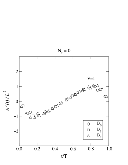
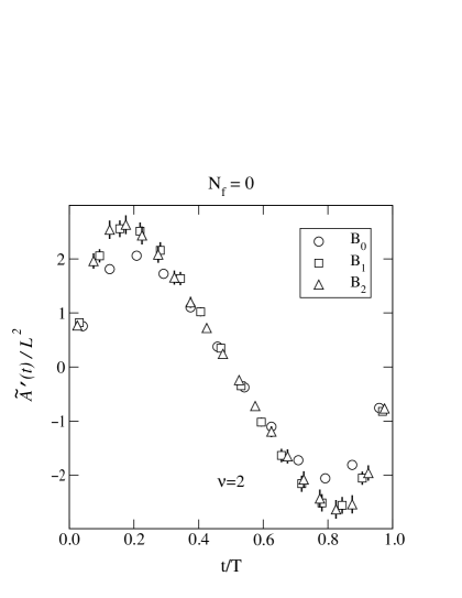
Figure 3: The numerical data corresponding to $\mathcal{A}^{\prime}(t)/L^{2}$, $\tilde{\mathcal{A}}^{\prime}(t)/L^{2}$, from the B lattices. Where not visible the statistical errors are smaller than the symbols. The left plot is for $|\nu|=1$, the right one for $|\nu|=2$. Comparing the slope at $t/T=0.5$ with the $\chi$PT predictions shown in Fig. 2, allows us to estimate $(FL)^{2}$.

From the zero-mode eigenfunctions, we compute the volume average of the correlators in Eqs. (2.7) and (2.8). There is a good signal in all cases, as illustrated in Fig. 3. Q$\chi$PT predicts that at non-zero times these correlators should behave like polynomials in time. We thus consider a Taylor expansion around the mid-point, $\tau=1/2$. Denoting $z\equiv\tau-1/2$, we define the coefficients $D_{\nu}$ and $C_{\nu}$ as

$$\frac{1}{L^{2}}\mathcal{A}^{\prime}(t) \equiv D_{\nu}\,z+C_{\nu}z^{3}+{\rm O}(z^{5})\;,$$ (3.9)

$$\frac{1}{L^{2}}\tilde{\mathcal{A}}^{\prime}(t) \equiv \tilde{D}_{\nu}\,z+\tilde{C}_{\nu}z^{3}+{\rm O}(z^{5})\;.$$ (3.10)

With a simple linear fit we can then extract the parameters $D_{\nu}$ and $C_{\nu}$ on jackknifed configurations. Table 2 shows the results of these fits in the time interval $(t_{\rm min},T/2)$. The data are modelled very well by the fits, and also the dependence on the choice of $t_{\rm min}$ is insignificant.

It is clear from Table 2 that only the $D_{\nu}$ coefficients can be extracted from the data in a reliable way. The errors on the $C_{\nu}$ coefficients are large and their central values vary quite significantly with the lattice spacing. This is to be expected since the $C_{\nu}$ coefficients are more relevant at short distances and so will also be more sensitive to cutoff effects. For this reason, we restrict ourselves to the $D_{\nu}$ coefficients in the following.

Lattice	$t_{\rm min}$	$z_{\mbox{\scriptsize min}}$	$D_{1}$	$D_{2}$	$\tilde{D}_{2}$	$C_{1}$	$C_{2}$	$\tilde{C}_{2}$
B0	$3a$	$0.208$	$3.7(1)$	$10.9(2)$	$-\phantom{1}9.1(4)$	$-\phantom{1}7(1)$	$-24(1)$	$19(3)$
B1	$4a$	$0.219$	$3.9(2)$	$10.8(4)$	$-11.1(9)$	$-\phantom{1}5(2)$	$-11(3)$	$26(8)$
B2	$5a$	$0.225$	$3.8(3)$	$10.7(4)$	$-\phantom{1}9.7(9)$	$-\phantom{1}3(3)$	$-13(4)$	$\phantom{1}8(8)$
C0	$4a$	$0.219$	$3.4(3)$	$\phantom{1}8.9(5)$	$-\phantom{1}9.2(9)$	$\phantom{-1}\,2(3)$	$-\phantom{1}4(5)$	$16(9)$
C1	$5a$	$0.225$	$3.9(5)$	$\phantom{1}9.4(7)$	$-\phantom{1}9.1(16)$	$-11(5)$	$\phantom{-1}7(7)$	$\phantom{1}2(19)$

Table 2: The $D_{\nu}$ and $C_{\nu}$ coefficients from the fit. The numbers in parentheses indicate the error of the last digit.

3.3 Analysis of the data

A Taylor expansion of the functions in Eqs. (3.7) and (3.8) and a matching with Eqs. (3.9) and (3.10) gives

$$D_{\nu} = \frac{2|\nu|}{(FL)^{2}}\biggl{\{}|\nu|+\frac{\alpha}{2N_{c}}-\frac{2KF}{\Sigma}-\frac{\beta_{1}}{F^{2}\sqrt{V}}$$ (3.11)

$$\hphantom{\frac{2|\nu|}{(FL)^{2}}\biggl{\{}}+\biggl{[}\biggl{(}{\frac{7}{3}}+2\nu^{2}-2\langle\nu^{2}\rangle\biggr{)}\zeta_{2}+{\frac{1}{2}}\gamma_{1}\biggr{]}\frac{T^{2}}{F^{2}V}\biggr{\}}\;,$$

$$\tilde{D}_{\nu} = \frac{2|\nu|}{(FL)^{2}}\biggl{\{}-1-|\nu|\biggl{(}\frac{\alpha}{2N_{c}}-\frac{2KF}{\Sigma}-\frac{\beta_{1}}{F^{2}\sqrt{V}}\biggr{)}$$ (3.12)

$$\hphantom{\frac{2|\nu|}{(FL)^{2}}\biggl{\{}}-|\nu|\biggl{[}\biggl{(}\frac{13}{3}-2\langle\nu^{2}\rangle\biggr{)}\zeta_{2}+{\frac{1}{2}}\gamma_{1}\biggr{]}\frac{T^{2}}{F^{2}V}\biggr{\}}\;,$$

where we have written $h_{2}^{\prime}(\tau)=\zeta_{2}z+{\rm O}(z^{3})$, $g_{1}^{\prime}(\tau)=\gamma_{1}z+{\rm O}(z^{3})$, and

$$\zeta_{2}=-\frac{1}{24}\;,\;\;\gamma_{1}=-\frac{1}{12}+{\frac{1}{2}}\sum_{{{\bf n}}\neq 0}\frac{1}{{\sinh}^{2}\left(|{{\bf p}}|/2\right)}\approx-0.0571276522\;,~{}~{}~{}\mbox{for $T=L$}\;,$$ (3.13)

with $|{{\bf p}}|=2\pi T[\sum_{i=1}^{3}n_{i}^{2}]^{1/2}/{L}$.

The quantity $\langle\nu^{2}\rangle$ in Eqs. (3.11) and (3.12) has recently been computed with high accuracy [8, 21]. In ref. [8] the results obtained at several lattice spacings were consistent with a well-defined continuum limit [33], giving $\hat{\chi}\equiv r_{0}^{4}\langle\nu^{2}\rangle/V=0.059(5)$, where $r_{0}=0.5$ fm [32]. In order to determine the other parameters $F,\alpha/N_{c}$, we need to fit for them simultaneously, but also take into account the error in the determination of $\hat{\chi}$. By comparing the results for the $D_{\nu}$ coefficients on the different lattices, cutoff effects are seen to be negligible within the statistical uncertainty. For this reason we do not attempt a continuum extrapolation here and simply consider the data at different lattice spacings as statistically independent. Since, on the other hand, the value of $\hat{\chi}$ cited above is the result of a continuum extrapolation, we will assign new error bars to it, large enough to also incorporate the finite lattice spacing values from [8]: $\hat{\chi}_{0}\equiv 0.059(10)$. We then perform a $\chi^{2}$ minimization in the three-parameter space $(F,\alpha/N_{c},\hat{\chi})$, with $\hat{\chi}$ added to the $\chi^{2}$ function as $\delta\chi^{2}=[(\hat{\chi}-\hat{\chi}_{0})/\delta\hat{\chi}_{0}]^{2}$.

We have performed three fits: the B lattices, the C lattices and their combination, taking into account the ratio of physical volumes, $L^{\mbox{\scriptsize({B})}}/L^{\mbox{\scriptsize({C})}}=16/20$. The values of $\chi^{2}_{\rm min}$ and the projections of the 68% confidence level contours onto the different parameter axes can be found in Table 3. The quality of the fits is good, with $\chi^{2}_{\rm min}/\mbox{dof}\mathop{\raise 1.29167pt\hbox{$<$\kern-7.5pt\raise-4.73611pt\hbox{$\sim$}}}1.0$ in all cases, and the B and C lattices give rather compatible results.

Lattice	dof	$\chi^{2}_{\rm min}$	$FL^{\mbox{\scriptsize({B})}}$	$\alpha/N_{c}$	$\hat{\chi}$
B	6	5.8	(0.84,0.92)	(0.3,1.2)	(0.04,0.08)
C	3	2.3	(0.76,1.01)	($-$0.6,2.6)	(0.04,0.08)
B+C	12	8.8	(0.83,0.90)	(0.3,0.9)	(0.05,0.08)

Table 3: Results from the global fits. The intervals are the projections of the 68% confidence level contours.

It is interesting to contrast this situation with what it would be in full QCD, where the $D_{\nu}$ coefficients only depend on the decay constant $F$:

$$D_{\nu} = +\frac{2|\nu|}{N_{\rm f}(FL)^{2}}\biggl{\{}(1+|\nu|N_{\rm f})\biggl{(}1-N_{\rm f}\frac{\beta_{1}}{F^{2}\sqrt{V}}\biggr{)}+\frac{T^{2}}{F^{2}V}\biggl{[}\gamma_{1}\biggl{(}\frac{2+N_{\rm f}^{2}}{2N_{\rm f}}+{4-N_{\rm f}^{2}\over 2}|\nu|\biggr{)}$$ (3.14)

$$+ \zeta_{2}\biggl{(}(6-N_{\rm f}^{2})|\nu|+{4\over N_{\rm f}}+N_{\rm f}(2\nu^{2}-1)\biggr{)}\biggr{]}\biggr{\}}\;,$$

$$\tilde{D}_{\nu} = -\frac{2|\nu|}{N_{\rm f}(FL)^{2}}\biggl{\{}(N_{\rm f}+|\nu|)\biggl{(}1-N_{\rm f}\frac{\beta_{1}}{F^{2}\sqrt{V}}\biggr{)}+\frac{T^{2}}{F^{2}V}\biggl{[}\gamma_{1}\biggl{(}{4-N_{\rm f}^{2}\over 2}+\frac{2+N_{\rm f}^{2}}{2N_{\rm f}}|\nu|\biggr{)}$$ (3.15)

$$+ \zeta_{2}\biggl{(}4+2\nu^{2}-N_{\rm f}^{2}+\frac{4}{N_{\rm f}}|\nu|+N_{\rm f}|\nu|\biggr{)}\biggr{]}\biggr{\}}\;.$$

These expressions show reasonable convergence (in the sense that the NNLO correction is less than 50% of the NLO term) only at $L\mathop{\raise 1.29167pt\hbox{$>$\kern-7.5pt\raise-4.73611pt\hbox{$\sim$}}}2.0$ fm for $F=93$ MeV, and in order to push the size of the correction below 30%, one would need to go to $L\mathop{\raise 1.29167pt\hbox{$>$\kern-7.5pt\raise-4.73611pt\hbox{$\sim$}}}2.5$ fm. In this case we might expect a systematic uncertainty in the determination of $F$ of about 5%, and statistical uncertainties would reach the same level if $D_{\nu}$ could be determined using $\sim 100$ configurations with $|\nu|=1$.

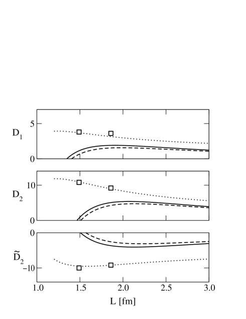
Figure 4: The coefficients $D_{1}$, $D_{2}$ and $\tilde{D}_{2}$ as a function of the box size for $N_{\rm f}=2$ (solid), $N_{\rm f}=3$ (dashed) and quenched (dotted). The quenched parameters are chosen at their best fit values according to Table 3, while $F=93$ MeV for $N_{\rm f}=2,3$. The symbols denote the averages of the data points from the B ($L^{\mbox{\scriptsize({B})}}=1.49$ fm) and C ($L^{\mbox{\scriptsize({C})}}=1.86$ fm) lattices.

The full theory formulae, Eqs. (3.14), (3.15), possess the feature that the NNLO corrections come with negative relative signs, such that the expressions are almost independent of $FL$ at around $FL\sim 1$, and their absolute values have an upper bound at this order. For illustration, we show the full predictions for $F=93$ MeV in Fig. 4, as a function of the box size (for a symmetric geometry, $L=T$). Also shown are the quenched data as well as the quenched predictions. Because of the mentioned near-cancellation, the full predictions at this order could not be moved significantly closer to the quenched data points by tuning $F$. In any case, as already mentioned, they show reasonable convergence and can thus be considered self-consistent predictions only for $L\mathop{\raise 1.29167pt\hbox{$>$\kern-7.5pt\raise-4.73611pt\hbox{$\sim$}}}2.0$ fm.

4 Conclusions

Approaching the chiral limit has remained a long-standing challenge for lattice QCD for many reasons, among them that finite-volume effects become large for very light pseudo-Goldstone bosons, and that the Dirac operator develops very small eigenvalues. It has been the purpose of this paper to elaborate on the fact that at least these particular problems can be overcome: for instance, the Dirac operator eigenfunctions associated with the exact zero modes encountered in gauge field configurations with a non-trivial topology at finite volume, can be used to extract physical information concerning the chiral limit of the infinite-volume theory.

More precisely, we have shown that certain classical scattering amplitudes of the zero-mode eigenfunctions measured at finite volumes, Eqs. (2.7), (2.8), allow the extraction of the infinite-volume pion decay constant, via the relations in Eq. (2.17). We have worked out these relations to NNLO, Eqs. (2.18), (2.19), finding that the convergence of chiral perturbation theory seems reasonable for these observables, provided the volume is above $\sim$ (2.0 fm)⁴.

Finally, to estimate the practical feasibility of using such relations, we have carried out lattice Monte Carlo simulations in the quenched approximation, using overlap fermions. We find a good signal for the observables in Eqs. (2.7), (2.8), shown in Fig. 3. Matching with chiral perturbation theory predictions relevant to the quenched approximation (which show reasonable apparent convergence only in volumes between $\sim$ (1.0 fm)⁴ and $\sim$ (2.0 fm)⁴, in marked contrast with the unquenched case), we find that the pion decay constant, to the extent that it is a well-defined quantity in this case, can be extracted with about 5% statistical accuracy, utilizing a few hundred configurations with non-trivial topology. The number we obtain in volumes $\sim$ (1.5 fm)⁴ is in the ballpark of 115 MeV.

Our result for the pion decay constant in the chiral limit is larger than what one would expect in Nature: conventional $\chi$PT in infinite volume [26] yields $F\approx 87$ MeV, if the standard phenomenological values for the ${\rm O}(p^{4})$ $L_{i}$ coefficients of Gasser and Leutwyler are inserted [34]. The fact that our quenched calculation seems to overestimate $F$ is consistent with other recent quenched results for the physical $F_{\pi}$ in the continuum limit, however [35]–[37]. For instance, the results of [35, 36] imply that the quenched $F_{\pi}$ is 10% larger than the experimental value, if the scale is set by $r_{0}$ [32]. On the other hand, these standard approaches (unlike ours) have to rely on quenched chiral extrapolations in the light quark masses, which introduce significant systematic uncertainties of their own [38].

On the side of our approach, it is conceivable that a smaller value for $F$ could be obtained by going to larger volumes. As we have discussed, however, the peculiarities of the quenched approximation imply that the volume cannot be increased too much, since the convergence of quenched chiral perturbation theory soon deteriorates. Therefore, a systematically improvable determination of $F$ by using our method (or any other) lies beyond the quenched approximation.

Appendix Appendix A Large-$N_{c}$ counting in the $\epsilon$-regime

Large-$N_{c}$ counting in the context of chiral perturbation theory has been analysed in detail in ref. [27]. The same general discussion goes through in the full and in the quenched theories, with the replacements in the latter that $U^{\dagger}\to U^{-1},e^{i\theta/N_{\rm f}}\to U_{\theta},{\rm Tr\,}\to{\rm Str\,}$. For simplicity, we will mostly use the notation of the unquenched theory here, indicating then the important point at which differences arise between the two cases.

In general, the chiral theory including the singlet is, at leading order in the momentum expansion and to all orders in $1/N_{c}$, of the form

$$\mathcal{L}_{\mbox{\scriptsize$\chi$PT}}\!\! = \!\!V_{0}(\Phi_{0})+V_{1}(\Phi_{0})~{}{\rm Tr\,}\Bigl{[}\partial_{\mu}U\partial_{\mu}U^{\dagger}\Bigr{]}$$ (A.1)

$$- \!\!\Bigl{\{}V_{2}(\Phi_{0}){\rm Tr\,}\!\Bigl{[}e^{i\theta/N_{\rm f}}UM\Bigr{]}+V_{2}^{*}(\Phi_{0}){\rm Tr\,}\!\Bigl{[}M^{\dagger}U^{\dagger}e^{-i\theta/N_{\rm f}}\Bigr{]}\Bigr{\}}+V_{3}(\Phi_{0})~{}(\partial_{\mu}\Phi_{0})^{2}+...\;,\hskip 25.6073pt$$

where $\Phi_{0}\equiv-i\frac{F}{2}{\rm Tr\,}\ln U$ and $M=\mathop{\mbox{diag}}(m,m,...)$.

The Lagrangian in Eq. (A.1) contains an infinite number of parameters, since the potentials $V_{i}(\Phi_{0})$ are arbitrary functions, with the only constraint from parity that $V_{i}(-\Phi_{0})=V_{i}(\Phi_{0})$, for $i=0,1,3$ and $V_{2}(-\Phi_{0})=V_{2}^{*}(\Phi_{0})$. It can be shown, however, that they involve a specific power series in $1/N_{c}$ ([25]–[27], and references therein). Noting that the field $\phi_{0}$ of [27] is $\phi_{0}=2\Phi_{0}/(\bar{F}\sqrt{N_{c}})$ in our notation below, the structures arising are

$$V_{0}(\Phi_{0}) \equiv {\frac{1}{2}}{m_{0}^{2}\over N_{c}}\Phi_{0}^{2}+{\rm O}\left({\Phi_{0}^{4}\over N^{4}_{c}}\right)\;,$$ (A.2)

$$V_{1}(\Phi_{0}) \equiv {N_{c}{\bar{F}}^{2}\over 4}+{\rm O}\left({\Phi_{0}^{2}\over N^{2}_{c}}\right)\;,$$ (A.3)

$$V_{2}(\Phi_{0}) \equiv {N_{c}{\bar{\Sigma}}\over 2}+i{\bar{K}\over\sqrt{N_{c}}}\Phi_{0}+{\rm O}\left({\Phi_{0}^{2}\over N^{2}_{c}}\right)\;,$$ (A.4)

$$V_{3}(\Phi_{0}) \equiv {\alpha\over 2N_{c}}+{\rm O}\left({\Phi_{0}^{2}\over N^{4}_{c}}\right)\;,$$ (A.5)

where all parameters introduced ($m_{0}^{2},\bar{F},\bar{\Sigma},\bar{K},\alpha$) are assumed not to scale with $N_{c}$. Inserting the specific terms shown here into Eq. (A.1), one obtains the theory up to ${\rm O}(1/N_{c})$. In the following, we denote

$$F^{2}\equiv{\bar{F}}^{2}N_{c},\quad\Sigma\equiv{\bar{\Sigma}}N_{c},\quad K\equiv\frac{\bar{K}}{\sqrt{N_{c}}}\;.$$ (A.6)

In order to define a formally consistent framework, it is convenient to now combine the momentum and $1/N_{c}$ expansions. Following [27], we may choose

$$p^{2}\sim\frac{1}{N_{c}}\sim\epsilon^{2}\;.$$ (A.7)

The defining property of the $\epsilon$-regime is that the pions are off-shell since the momenta are fixed by the size of the box, $p\sim 1/L\sim{\rm O}(\epsilon)$, while the quark mass is small, such that

$$\mu\equiv m\Sigma V\mathop{\raise 1.29167pt\hbox{$<$\kern-7.5pt\raise-4.73611pt\hbox{$\sim$}}}1\;.$$ (A.8)

Given Eqs. (A.6), (A.7), we are thus led to the rule

$$m\sim\epsilon^{6}\;.$$ (A.9)

As usual, the field configurations are factorized into zero-momentum modes $U_{0},\bar{\Phi}_{0}$ and non-zero modes $\xi,\tilde{\Phi}_{0}$,

$$U(x)=U_{\xi}(x)U_{0}\;,\quad U_{\xi}(x)=\exp\left[\frac{2i\xi(x)}{F}\right]\;,\quad\Phi_{0}(x)=\tilde{\Phi}_{0}(x)+\bar{\Phi}_{0}\;,$$ (A.10)

where $\int\!{\rm d}^{4}x\,\xi(x)=0$ and $\tilde{\Phi}_{0}={\rm Tr\,}\xi$. The counting rules for the non-zero modes, which are treated perturbatively, are

$$\xi\sim p\sim\epsilon\;,\quad\tilde{\Phi}_{0}\sim p\sim\epsilon\;.$$ (A.11)

For the zero mode $U_{0}$ we have $U_{0}\sim 1$, while the counting of $\bar{\Phi}_{0}$ is to be determined presently.

Indeed, let us consider the terms involving explicitly the flavour singlet zero mode $\bar{\Phi}_{0}$. We are interested in carrying out the computation up to and including ${\rm O}(\epsilon^{4})$, and the terms potentially of this order, after integration over space-time, are

$$\int\!{\rm d}^{4}x\,\mathcal{L}_{\mbox{\scriptsize$\chi$PT}} \ni +{\frac{1}{2}}\frac{m_{0}^{2}}{N_{c}}V\bar{\Phi}_{0}^{2}~{}~{}\sim~{}~{}{\rm O}(m_{0}^{2}){\rm O}(\bar{\Phi}_{0}^{2}){\rm O}(\epsilon^{-2})\;,$$ (A.13)

$$-i\,mKV\,\bar{\Phi}_{0}{\rm Tr\,}\Bigl{[}e^{i\theta/N_{\rm f}}U_{0}-U_{0}^{\dagger}e^{-i\theta/N_{\rm f}}\Bigr{]}~{}~{}\sim~{}~{}{\rm O}(\bar{K}){\rm O}(\bar{\Phi}_{0}){\rm O}(\epsilon^{3})\;.\hskip 14.22636pt$$

Moreover, we want to carry out the computation at a fixed topology; performing the integral over $\theta$ with the weight $\exp(i\theta\nu)$ introduces (after a shift) effectively one more term,

$$\int\!{\rm d}^{4}x\,\mathcal{L}_{\mbox{\scriptsize$\chi$PT}}~{}~{}\ni~{}~{}\frac{2i\nu}{F}\bar{\Phi}_{0}~{}~{}\sim~{}~{}{\rm O}(\bar{\Phi}_{0}){\rm O}(\epsilon)\;.$$ (A.14)

Once the integral over $\theta$ is converted to a Gaussian over $\bar{\Phi}_{0}$, Eqs. (A.13), (A.14) tell that the saddle point is at leading order in $\epsilon$ at $\bar{\Phi}_{0}\sim N_{c}\nu/(m_{0}^{2}FV)\sim{\rm O}(\epsilon^{3})/{\rm O}(m_{0}^{2})$. Thus, we have fixed also the counting of $\bar{\Phi}_{0}$.

We can now collect together the full theory at fixed topology. The factorized part of the zero-mode partition function becomes

$$Z_{\nu}(\mu) \propto e^{-\frac{\nu^{2}}{2\langle\nu^{2}\rangle}}\int_{\mbox{\scriptsize$U_{0}\in$ U($N_{\rm f}$)}}{\det}^{\nu}U_{0}\,\exp\Bigl{[}{\,\frac{\mu}{2}{\rm Tr\,}(U_{0}+U_{0}^{\dagger})+2\nu\frac{mKN_{c}}{m_{0}^{2}F}{\rm Tr\,}(U_{0}-U_{0}^{\dagger})}\Bigr{]}\;,\hskip 14.22636pt$$ (A.15)

where

$$\frac{\langle\nu^{2}\rangle}{V}=\frac{m_{0}^{2}F^{2}}{4N_{c}}\;.$$ (A.16)

The first term in the exponent is ${\rm O}(1)$, while the latter is, as follows from Eq. (A.13) with the given estimate of $\bar{\Phi}_{0}$, $\sim{\rm O}(\bar{K}){\rm O}(\epsilon^{6})/{\rm O}(m_{0}^{2})$. The non-zero momentum modes, on the other hand, are described by

$$\int\!{\rm d}^{4}x\,\mathcal{L}_{\mbox{\scriptsize$\chi$PT}} \ni +\int\!{\rm d}^{4}x\,\frac{F^{2}}{4}{\rm Tr\,}\Bigl{[}\partial_{\mu}U_{\xi}\partial_{\mu}U_{\xi}^{\dagger}\Bigr{]}~{}~{}\sim~{}~{}{\rm O}(\epsilon^{0})\Bigl{[}1+{\rm O}(\epsilon^{4})\Bigr{]}\;,$$ (A.20)

$$-\int\!{\rm d}^{4}x\,\frac{m\Sigma}{2}\left.{\rm Tr\,}\Bigl{[}U_{\xi}U_{0}+U_{0}^{\dagger}U_{\xi}^{\dagger}\Bigr{]}\right|_{{\rm O}(\xi^{2})}~{}~{}\sim~{}~{}{\rm O}(\epsilon^{4})\;,$$

$$+\int\!{\rm d}^{4}x\,\frac{\alpha}{2N_{c}}\Bigl{(}\partial_{\mu}\tilde{\Phi}_{0}\Bigr{)}^{2}~{}~{}\sim~{}~{}{\rm O}(\alpha){\rm O}(\epsilon^{2})\;,$$

$$+\int\!{\rm d}^{4}x\,\frac{m_{0}^{2}}{2N_{c}}\tilde{\Phi}_{0}^{2}~{}~{}\sim~{}~{}{\rm O}(m_{0}^{2}){\rm O}(\epsilon^{0})\;.$$

To finalize the setup, one has to decide what kind of counting rules are chosen for the parameters $m_{0}^{2},\alpha,\bar{K}$. For simplicity, we will assume that ${\rm O}(\alpha)\sim{\rm O}(\bar{K})\sim 1$. The counting of $m_{0}^{2}$ then leads to three distinct possibilities:

• In the unquenched theory, $m_{0}^{2}$ can be taken as “large”, say $m_{0}^{2}\sim\epsilon^{-2}$. Parametrically, then, $m_{0}^{2}/N_{c}\gg p^{2}$. In this case the term in Eq. (A.20) dominates the action: the non-zero modes $\tilde{\Phi}_{0}$ (representing the $\eta^{\prime}$) are heavy and can be integrated out, resulting in the simple usual chiral theory following from Eq. (2.10).

  This choice is not available in the quenched limit, however: the field $\tilde{\Phi}_{0}$ cannot be integrated out [23, 24], but has to be treated as a light degree of freedom. Therefore, it is convenient to assign a different counting to it.

• In the “standard” version of quenched chiral perturbation theory, one chooses $m_{0}^{2}\sim{\rm O}(1)$, such that $m_{0}^{2}/N_{c}\sim p^{2}$ [29]. Then Eq. (A.20) is of the same order as the usual kinetic terms following from Eq. (A.20). The term with $K$ in Eq. (A.15), on the other hand, can be neglected, since it is ${\rm O}(\epsilon^{6})$ with this counting.

  This standard counting suffers from some problems, however. First of all, the integrals over the graded group of the supersymmetric formulation do not appear to be, strictly speaking, well defined [29], because the masses related to quadratic fluctuations, treated according to Zirnbauer’s prescription [28], are not positive-definite (cf. Eq. (3.8) in [29]). Second, Q$\chi$PT leads to a perturbative expansion parameter $\sim m_{0}^{2}/(N_{c}p^{2})$. With the standard counting this is of order unity, formally spoiling the convergence.

• Because of the problems of the standard counting, we will consider an “alternative” counting here. In the alternative counting, $m_{0}^{2}$ is treated as a small quantity, say $m_{0}^{2}\sim\epsilon^{2}$. Then Eq. (A.20) is formally a perturbation and the leading order quadratic form is well defined. This counting makes also explicit the fact that Q$\chi$PT should only work in the window of Eq. (3.3). With the choice $m_{0}^{2}\sim\epsilon^{2}$, contributions from the coefficient $K$ should be kept in the results.

In the real world, obviously, $1/N_{c}$ is not tunable, and not necessarily small. Therefore, the success or failure of the frameworks described remains ultimately to be judged empirically, by comparing them with data. The expressions below are, for generality, for the “standard counting”, while in the actual text we only showed truncated versions, where terms of higher order according to the “alternative counting” had been dropped.

Appendix Appendix B Detailed results for full chiral perturbation theory

B.1 Space-time integrals appearing

After integration over the spatial volume, the time dependence of Eq. (2.13) appears in the forms

$$\int\!{\rm d}^{3}{\bf x}\, = L^{3}\;,$$ (B.1)

$$\int\!{\rm d}^{3}{\bf x}\,G(x) = Th_{1}(\tau)\;,$$ (B.2)

$$\int\!{\rm d}^{3}{\bf x}\,\Bigl{[}G(x)\Bigr{]}^{2} = \frac{T^{2}}{L^{3}}g_{1}(\tau)\;,$$ (B.3)

$$\int\!{\rm d}^{3}{\bf x}\,\int\!{\rm d}^{4}y\,G(x-y)G(y) = -T^{3}h_{2}(\tau)\;,$$ (B.4)

where

$$h_{1}(\tau) \equiv \frac{1}{2}\left[\left(\tau-{1\over 2}\right)^{2}-{1\over 12}\right]\;,$$ (B.5)

$$h_{2}(\tau) \equiv \frac{1}{24}\left[\tau^{2}\left(\tau-1\right)^{2}-{1\over 30}\right]\;,$$ (B.6)

$$g_{1}(\tau) \equiv [h_{1}(\tau)]^{2}+\sum_{{{\bf n}}\neq 0}\left[{{\cosh}\left(|{{\bf p}}|(\tau-1/2)\right)\over 2|{{\bf p}}|{\sinh}\left(|{{\bf p}}|/2\right)}\right]^{2}\;.$$ (B.7)

Here

$$|{{\bf p}}|=2\pi\frac{T}{L}\left[\sum_{i=1}^{3}n_{i}^{2}\right]^{1/2}\;.$$ (B.8)

B.2 Zero-mode integrals appearing

The zero-momentum mode integrals at fixed topology are related to the partition function

$$Z_{\nu}(\mu)\equiv\int_{U_{0}\in{\rm U}(N_{\rm f})}{\det}^{\nu}U_{0}\,e^{\,\mu\mathop{\rm Re}{\rm Tr\,}U_{0}}\;,$$ (B.9)

where $\mu=m\Sigma V$. The value of $Z_{\nu}(\mu)$ is known [39, 18] to be

$$Z_{\nu}(\mu)=\det[I_{\nu+j-i}(\mu)],$$ (B.10)

where the determinant is taken over an $N_{\rm f}\times N_{\rm f}$ matrix, whose matrix element $(i,j)$ is the modified Bessel function $I_{\nu+j-i}$. We will express our results in terms of the derivatives of this partition function, in particular

$$\sigma_{\nu}(\mu)\equiv\frac{\Sigma_{\nu}(\mu)}{\Sigma}\equiv\frac{1}{N_{\rm f}}\frac{\partial}{\partial\mu}\ln Z_{\nu}(\mu)\;.$$ (B.11)

At small $\mu$ and non-zero $\nu$,

$$\sigma_{\nu}(\mu)\approx\frac{|\nu|}{\mu}\;.$$ (B.12)

Expectation values are denoted by

$$\langle...\rangle^{\mu}_{\nu}\equiv\frac{\int_{U_{0}\in{\rm U}(N_{\rm f})}(...)\det^{\nu}\!U_{0}\,e^{\,\mu\mathop{\rm Re}{\rm Tr\,}U_{0}}}{\int_{U_{0}\in{\rm U}(N_{\rm f})}\det^{\nu}\!U_{0}\,e^{\,\mu\mathop{\rm Re}{\rm Tr\,}U_{0}}}\;;$$ (B.13)

both the superscript and subscript in $\langle...\rangle^{\mu}_{\nu}$ are often left out.

Given these definitions, all the emerging expectation values can be computed analytically, using the techniques discussed in Appendix B of [29]. The small-$\mu$ (small-$m$) limits are then obtained by using Eq. (B.12). We give here a complete collection of the integrals appearing, up to third order in the matrices $U_{0},U_{0}^{\dagger}$. The expectation values for complex-conjugated operators are obtained from those shown simply by $\nu\to-\nu$. For the small-$\mu$ limits we only show the values of order $1/\mu^{n}$, for $n$ powers of $U_{0},U_{0}^{\dagger}$:

$$\langle{\rm Tr\,}U_{0}\rangle = N_{\rm f}\Bigl{[}\sigma_{\nu}-\frac{\nu}{\mu}\Bigr{]}$$ (B.14)

$$\approx \frac{N_{\rm f}}{\mu}(|\nu|-\nu)\;,$$ (B.15)

$$\langle{\rm Tr\,}(U_{0}^{2})\rangle = N_{\rm f}\Bigl{[}1-\frac{2(N_{\rm f}+\nu)}{\mu}\Bigl{(}\sigma_{\nu}-\frac{\nu}{\mu}\Bigr{)}\Bigr{]}$$ (B.16)

$$\approx -\frac{2N_{\rm f}}{\mu^{2}}(N_{\rm f}+\nu)(|\nu|-\nu)\;,$$ (B.17)

$$\langle{\rm Tr\,}U_{0}{\rm Tr\,}U_{0}^{\dagger}\rangle = N_{\rm f}\Bigl{[}\sigma_{\nu}^{\prime}+N_{\rm f}\sigma_{\nu}^{2}+\frac{\sigma_{\nu}}{\mu}-N_{\rm f}\frac{\nu^{2}}{\mu^{2}}\Bigr{]}$$ (B.18)

$$\approx 0\times\frac{N_{\rm f}}{\mu^{2}}\;,$$ (B.19)

$$\langle({\rm Tr\,}U_{0})^{2}\rangle = N_{\rm f}\Bigl{[}\sigma_{\nu}^{\prime}+N_{\rm f}\sigma_{\nu}^{2}-(1+2N_{\rm f}\nu)\frac{\sigma_{\nu}}{\mu}+(2+N_{\rm f}\nu)\frac{\nu}{\mu^{2}}\Bigr{]}$$ (B.20)

$$\approx -\frac{2N_{\rm f}}{\mu^{2}}(1+N_{\rm f}\nu)(|\nu|-\nu)\;,$$ (B.21)

$$\langle{\rm Tr\,}(U_{0}^{3})\rangle = N_{\rm f}\biggl{\{}-\frac{2\nu}{\mu^{3}}(2\nu^{2}+5N_{\rm f}\nu+2N_{\rm f}^{2}+2)-\frac{1}{\mu}(2N_{\rm f}+3\nu)$$ (B.22)

$$+\Bigl{[}1+\frac{2}{\mu^{2}}(2\nu^{2}+6N_{\rm f}\nu+2N_{\rm f}^{2}+1)\Bigr{]}\sigma_{\nu}-\frac{2}{\mu}(\sigma_{\nu}^{\prime}+N_{\rm f}\sigma_{\nu}^{2})\biggr{\}}$$

$$\approx \frac{4N_{\rm f}}{\mu^{3}}(1+N_{\rm f}^{2}+3N_{\rm f}\nu+\nu^{2})(|\nu|-\nu)\;,$$ (B.23)

$$\langle{\rm Tr\,}U_{0}{\rm Tr\,}(U_{0}^{2})\rangle = N_{\rm f}\biggl{\{}-\frac{2\nu}{\mu^{3}}\Bigl{[}(4+N_{\rm f}^{2})\nu+N_{\rm f}(4+\nu^{2})\Bigr{]}-\frac{2+N_{\rm f}\nu}{\mu}$$ (B.24)

$$+\Bigl{[}N_{\rm f}+\frac{2}{\mu^{2}}\Bigl{(}(3+2N_{\rm f}^{2})\nu+N_{\rm f}(3+2\nu^{2})\Bigr{)}\Bigr{]}\sigma_{\nu}$$

$$-2\frac{N_{\rm f}+\nu}{\mu}(\sigma_{\nu}^{\prime}+N_{\rm f}\sigma_{\nu}^{2})\biggr{\}}$$

$$\approx \frac{4N_{\rm f}}{\mu^{3}}\Bigl{[}2N_{\rm f}+(2+N_{\rm f}^{2})\nu+N_{\rm f}\nu^{2}\Bigr{]}(|\nu|-\nu)\;,$$ (B.25)

$$\langle{\rm Tr\,}U_{0}^{\dagger}{\rm Tr\,}(U_{0}^{2})\rangle = N_{\rm f}\biggl{\{}\frac{2N_{\rm f}\nu^{2}}{\mu^{3}}(N_{\rm f}+\nu)+\frac{2+N_{\rm f}\nu}{\mu}$$ (B.26)

$$+\Bigl{[}N_{\rm f}-\frac{2}{\mu^{2}}(N_{\rm f}+\nu)\Bigr{]}\sigma_{\nu}-\frac{2(N_{\rm f}+\nu)}{\mu}(\sigma_{\nu}^{\prime}+N_{\rm f}\sigma_{\nu}^{2})\biggr{\}}$$

$$\approx 0\times\frac{N_{\rm f}}{\mu^{3}}\;,$$ (B.27)

$$\langle({\rm Tr\,}U_{0})^{3}\rangle = N_{\rm f}\Bigl{[}-\frac{\nu}{\mu^{3}}(8+6N_{\rm f}\nu+N_{\rm f}^{2}\nu^{2})+\frac{3}{\mu^{2}}(1+3N_{\rm f}\nu+N_{\rm f}^{2}\nu^{2})\sigma_{\nu}$$ (B.28)

$$-\frac{3}{\mu}(1+N_{\rm f}\nu)(\sigma_{\nu}^{\prime}+N_{\rm f}\sigma_{\nu}^{2})+\sigma_{\nu}^{\prime\prime}+3N_{\rm f}\sigma_{\nu}^{\prime}\sigma_{\nu}+N_{\rm f}^{2}\sigma_{\nu}^{3}\Bigr{]}$$

$$\approx \frac{4N_{\rm f}}{\mu^{3}}(2+3N_{\rm f}\nu+N_{\rm f}^{2}\nu^{2})(|\nu|-\nu)\;,$$ (B.29)

$$\langle({\rm Tr\,}U_{0}^{\dagger})({\rm Tr\,}U_{0})^{2}\rangle = N_{\rm f}\Bigl{[}N_{\rm f}\frac{\nu^{2}}{\mu^{3}}(2+N_{\rm f}\nu)-\frac{1}{\mu^{2}}(1+N_{\rm f}\nu+N_{\rm f}^{2}\nu^{2})\sigma_{\nu}$$ (B.30)

$$+\frac{1-N_{\rm f}\nu}{\mu}(\sigma_{\nu}^{\prime}+N_{\rm f}\sigma_{\nu}^{2})+\sigma_{\nu}^{\prime\prime}+3N_{\rm f}\sigma_{\nu}^{\prime}\sigma_{\nu}+N_{\rm f}^{2}\sigma_{\nu}^{3}\Bigr{]}$$

$$\approx 0\times\frac{N_{\rm f}}{\mu^{3}}\;.$$ (B.31)

It may be noted from the small-$\mu$ expressions that plenty of degeneracies emerge if we put $N_{\rm f}\to 1$: this is simply because taking a trace has then no meaning.

B.3 Results for the coefficients in Eq. (2.13)

Let us define

$$\Sigma^{\prime}\equiv\Sigma\biggl{[}1-\frac{N_{\rm f}^{2}-1}{N_{\rm f}}\frac{G(0)}{F^{2}}\biggr{]}=\Sigma\biggl{[}1+\frac{N_{\rm f}^{2}-1}{N_{\rm f}}\frac{\beta_{1}}{F^{2}\sqrt{V}}\biggr{]}\;,$$ (B.32)

and

$$\mu^{\prime}\equiv m\Sigma^{\prime}V\;.$$ (B.33)

For the coefficient $C_{I}$ defined in Eq. (2.13), we then obtain (at NLO)

$$C_{I}=-{\frac{1}{4}}\Bigl{(}\Sigma^{\prime}\Bigr{)}^{2}\Bigl{\langle}\Bigl{\{}{\rm Tr\,}\Bigl{[}T^{I}(U_{0}-U_{0}^{\dagger})\Bigr{]}\Bigr{\}}^{2}\Bigr{\rangle}^{\mu^{\prime}}_{\nu}\;,$$ (B.34)

where $I$ is not summed over. For $I=0$ (flavour singlet), the result is immediately related to the expectation values listed in Eqs. (B.14)–(B.31); for $I=a$, one can make the connection by using independence of $a$ and the completeness relation

$$\langle T^{a}_{ij}T^{a}_{kl}F_{ijkl}\rangle=\frac{1}{N_{\rm f}^{2}-1}\sum_{a=1}^{N_{\rm f}^{2}-1}\langle T^{a}_{ij}T^{a}_{kl}F_{ijkl}\rangle=\frac{1}{2(N_{\rm f}^{2}-1)}\Bigl{\langle}F_{ijji}-\frac{1}{N_{\rm f}}F_{iijj}\Bigr{\rangle}\;.$$ (B.35)

We show explicitly only the small-$\mu$ limits here:

$$C_{0} = \frac{\Sigma^{2}N_{\rm f}|\nu|}{\mu^{2}}(1-N_{\rm f}|\nu|)\;,$$ (B.36)

$$C_{a} = \frac{\Sigma^{2}|\nu|}{2\mu^{2}}\;.$$ (B.37)

For $\alpha_{I}$, we obtain, in a similar way,

$$\alpha_{I} = \frac{\Sigma^{2}}{2F^{2}}\biggl{[}1-\frac{N_{\rm f}^{2}-2}{N_{\rm f}}\frac{G(0)}{F^{2}}\biggr{]}\times$$ (B.38)

$$\times\biggl{\langle}{\rm Tr\,}\Bigl{[}(U_{0}T^{I}+T^{I}U_{0}^{\dagger})^{2}\Bigr{]}-\frac{1}{N_{\rm f}}\Bigl{\{}{\rm Tr\,}\Bigl{[}T^{I}(U_{0}+U_{0}^{\dagger})\Bigr{]}\Bigr{\}}^{2}\biggr{\rangle}^{\mu^{\prime}}_{\nu}\;.$$

For small $\mu$,

$$\alpha_{0} = \frac{2\Sigma^{2}|\nu|}{F^{2}\mu^{2}}\biggl{[}1+N_{\rm f}\frac{G(0)}{F^{2}}\biggr{]}(1-N_{\rm f}^{2})\;,$$ (B.39)

$$\alpha_{a} = \frac{\Sigma^{2}|\nu|}{F^{2}\mu^{2}N_{\rm f}}\biggl{[}1+N_{\rm f}\frac{G(0)}{F^{2}}\biggr{]}(1+N_{\rm f}|\nu|)\;.$$ (B.40)

For $\beta_{I}$, we obtain

$$\beta_{I}=-\frac{\Sigma^{2}}{F^{4}}\biggl{\langle}\frac{N_{\rm f}^{2}+2}{4N_{\rm f}^{2}}\Bigl{\{}{\rm Tr\,}\Bigl{[}T^{I}(U_{0}-U_{0}^{\dagger})\Bigr{]}\Bigr{\}}^{2}+\frac{N_{\rm f}^{2}-4}{4N_{\rm f}}{\rm Tr\,}\Bigl{[}(U_{0}T^{I}-T^{I}U_{0}^{\dagger})^{2}\Bigr{]}\biggr{\rangle}^{\mu}_{\nu}\;.$$ (B.41)

For small $\mu$,

$$\beta_{0} = \frac{\Sigma^{2}|\nu|}{F^{4}\mu^{2}N_{\rm f}}(N_{\rm f}^{2}-1)(N_{\rm f}^{2}-2-2N_{\rm f}|\nu|)\;,$$ (B.42)

$$\beta_{a} = \frac{\Sigma^{2}|\nu|}{2F^{4}\mu^{2}N_{\rm f}^{2}}\Bigl{[}N_{\rm f}^{2}+2-N_{\rm f}(N_{\rm f}^{2}-4)|\nu|\Bigr{]}\;.$$ (B.43)

Finally, $\gamma_{I}$ reads

$$\gamma_{I} = \frac{\Sigma^{2}}{2F^{4}V}\biggl{\langle}\Bigl{\{}{\rm Tr\,}\Bigl{[}T^{I}(U_{0}+U_{0}^{\dagger})\Bigr{]}\Bigr{\}}^{2}-N_{\rm f}{\rm Tr\,}\Bigl{[}(U_{0}T^{I}+T^{I}U_{0}^{\dagger})^{2}\Bigr{]}$$ (B.44)

$$-\mu{\rm Tr\,}\Bigl{[}(U_{0}+U_{0}^{\dagger})(U_{0}T^{I}+T^{I}U_{0}^{\dagger})^{2}\Bigr{]}$$

$$+\frac{2\mu}{N_{\rm f}}{\rm Tr\,}\Bigl{[}(U_{0}+U_{0}^{\dagger})(U_{0}T^{I}+T^{I}U_{0}^{\dagger})\Bigr{]}{\rm Tr\,}\Bigl{[}T^{I}(U_{0}+U_{0}^{\dagger})\Bigr{]}$$

$$-\frac{\mu}{N_{\rm f}^{2}}{\rm Tr\,}(U_{0}+U_{0}^{\dagger})\Bigl{\{}{\rm Tr\,}\Bigl{[}T^{I}(U_{0}+U_{0}^{\dagger})\Bigr{]}\Bigr{\}}^{2}\biggr{\rangle}^{\mu}_{\nu}\;.$$

For small $\mu$,

$$\gamma_{0} = -\frac{2\Sigma^{2}|\nu|}{F^{4}V\mu^{2}N_{\rm f}}(N_{\rm f}^{2}-1)(N_{\rm f}^{2}-4-2N_{\rm f}|\nu|)\;,$$ (B.45)

$$\gamma_{a} = \frac{\Sigma^{2}|\nu|}{F^{4}V\mu^{2}N_{\rm f}^{2}}\Bigl{[}N_{\rm f}^{2}(1-2\nu^{2})-4+N_{\rm f}(N_{\rm f}^{2}-6)|\nu|\Bigr{]}\;.$$ (B.46)

Appendix Appendix C Detailed results for quenched chiral perturbation theory

C.1 Additional space-time integrals in the quenched theory

Apart from the integrals in Eqs. (B.1)–(B.4), Eqs. (3.1) and (3.5) imply that in the quenched case we need, in general, the following further ones:

$$\int\!{\rm d}^{3}{\bf x}\,F(x) = -T^{3}h_{2}(\tau)\;,$$ (C.1)

$$\int\!{\rm d}^{3}{\bf x}\,G(x)F(x) = \frac{T^{4}}{L^{3}}g_{2}(\tau)\;,$$ (C.2)

$$\int\!{\rm d}^{3}{\bf x}\,\Bigl{[}F(x)\Bigr{]}^{2} = \frac{T^{6}}{L^{3}}g_{3}(\tau)\;,$$ (C.3)

$$\int\!{\rm d}^{3}{\bf x}\int\!{\rm d}^{4}y\,G(x-y)F(y) = T^{5}h_{3}(\tau)\;,$$ (C.4)

$$\int\!{\rm d}^{3}{\bf x}\int\!{\rm d}^{4}y\,F(x-y)F(y) = -T^{7}h_{4}(\tau)\;,$$ (C.5)

where we have defined (following the notation in Eqs. (B.5)–(B.8)),

$$h_{3}(\tau) \equiv \frac{1}{720}\left[\tau^{2}\left(\tau-1\right)^{2}\left(\tau(\tau-1)-{1\over 2}\right)+{1\over 42}\right]\;,$$ (C.6)

$$h_{4}(\tau) \equiv \frac{1}{120960}\left[\tau^{2}\left(\tau-1\right)^{2}\left(3\tau^{4}-6\tau^{3}-\tau^{2}+4\tau+2\right)-{1\over 10}\right]\;,$$ (C.7)

$$g_{2}(\tau) \equiv -h_{1}(\tau)h_{2}(\tau)-\sum_{{{\bf n}}\neq 0}{{\cosh}\left(|{{\bf p}}|(\tau-1/2)\right)\over 2|{{\bf p}}|{\sinh}\left(|{{\bf p}}|/2\right)}{1\over 2|{{\bf p}}|}{{\rm d}\over{\rm d}|{{\bf p}}|}\left({{\cosh}\left(|{{\bf p}}|(\tau-1/2)\right)\over 2|{{\bf p}}|{\sinh}\left(|{{\bf p}}|/2\right)}\right)\;,\hskip 14.22636pt$$ (C.8)

$$g_{3}(\tau) \equiv [h_{2}(\tau)]^{2}+\sum_{{{\bf n}}\neq 0}\left[{1\over 2|{{\bf p}}|}{{\rm d}\over{\rm d}|{{\bf p}}|}\left({{\cosh}\left(|{{\bf p}}|(\tau-1/2)\right)\over 2|{{\bf p}}|{\sinh}\left(|{{\bf p}}|/2\right)}\right)\right]^{2}\;.$$ (C.9)

C.2 Quenched zero-mode integrals for the flavour singlets

As discussed in the main text, in the quenched case, the results for the flavour non-singlet follow from those for the flavour singlet. Therefore, we only need to address the zero-mode integrals arising for the flavour singlets, and do not present a similarly exhaustive list as in Appendix B.2.

The flavour singlets contain two parts, a connected contraction ($\propto N_{\rm v}$) and a disconnected one ($\propto N_{\rm v}^{2}$). The replica trick (cf. [30]) allows to obtain the result for the connected contraction from a certain limit of U($N_{\rm f}$) integrals, discussed in Appendix B.2. For the disconnected contraction, on the other hand, the zero-mode integrals have to be honestly carried out, for $N_{\rm v}=1$, using the supersymmetric formulation of Q$\chi$PT. (The non-zero momentum modes of the Goldstone bosons can still be treated with the replica formulation [31], and only the remaining zero-momentum mode integrals need to be transformed to the supersymmetric ones.) We first list the supersymmetric integrals for $N_{\rm v}=1$, and then the generalizations to any $N_{\rm v}$ obtained with the replica trick.

Let us start with some notation. We introduce a projection operator $P_{\rm v}$,

$$(P_{\rm v})_{ij}\equiv\left\{\begin{array}[]{ll}\delta_{ij},&\mbox{for $i,j$ = physical flavours in the valence block,}\\ 0,&\mbox{otherwise.}\end{array}\right.$$ (C.10)

Using again the scaling variable $\mu\equiv m\Sigma V$, all mass dependence of the results can be expressed in terms the same zero-mode integral as appears in the quark condensate obtained with $\widehat{\rm Gl}(1|1)$ [40]:

$$\frac{1}{2N_{\rm v}}\langle{\rm Str\,}[P_{\rm v}(U_{0}+U_{0}^{-1})]\rangle\equiv\sigma_{\nu}\equiv{\Sigma_{\nu}(\mu)\over\Sigma}=\mu\Bigl{[}I_{\nu}(\mu)K_{\nu}(\mu)+I_{\nu+1}(\mu)K_{\nu-1}(\mu)\Bigr{]}+{\nu\over\mu}\;,$$ (C.11)

where $I_{\nu},K_{\nu}$ are modified Bessel functions. We recall that, for $\nu\neq 0$,

$$\sigma_{\nu}(\mu)\approx\frac{|\nu|}{\mu}\;,$$ (C.12)

as in Eq. (B.12). Note that, in contrast to Eq. (C.11),

$$\langle{\rm Str\,}(U_{0}+U_{0}^{-1})\rangle=0\;,$$ (C.13)

and also that $\langle{\rm Str\,}(U_{0}-U_{0}^{-1})\rangle=0$.

The zero-mode integrals for $N_{\rm v}=1$ can be derived following the techniques discussed in [29], particularly the explicit parametrization of $\widehat{\rm Gl}(1|1)$. The integrals needed, and their small-$\mu$ limits, read ($U\equiv U_{0}$ here)

$$\Bigl{\langle}(U_{11})^{2}+(U^{-1}_{11})^{2}\Bigr{\rangle} = 2\Bigl{[}\sigma_{\nu}^{\prime}-\frac{\sigma_{\nu}}{\mu}+1+\frac{2\nu^{2}}{\mu^{2}}\Bigr{]}$$ (C.14)

$$\approx \frac{4|\nu|}{\mu^{2}}(|\nu|-1)\;,$$ (C.15)

$$\Bigl{\langle}(U_{11})^{2}-(U^{-1}_{11})^{2}\Bigr{\rangle} = \frac{4\nu}{\mu}\Bigl{[}\frac{1}{\mu}-\sigma_{\nu}\Bigr{]}$$ (C.16)

$$\approx \frac{4\nu}{\mu^{2}}(1-|\nu|)\;,$$ (C.17)

$$\Bigl{\langle}U_{11}U^{-1}_{11}\Bigr{\rangle} = \sigma_{\nu}^{\prime}+\frac{\sigma_{\nu}}{\mu}+1$$ (C.18)

$$\approx 0\times\frac{1}{\mu^{2}}\;,$$ (C.19)

$$\Bigl{\langle}(U_{11})^{3}+(U^{-1}_{11})^{3}\Bigr{\rangle} = \sigma_{\nu}^{\prime\prime}-7\frac{\sigma_{\nu}^{\prime}}{\mu}+\sigma_{\nu}\Bigl{[}2+\frac{7+8\nu^{2}}{\mu^{2}}\Bigr{]}-\frac{6}{\mu}-\frac{24\nu^{2}}{\mu^{3}}\hskip 22.76228pt$$ (C.20)

$$\approx \frac{8|\nu|}{\mu^{3}}(|\nu|-1)(|\nu|-2)\;,$$ (C.21)

$$\Bigl{\langle}(U_{11})^{2}U^{-1}_{11}+U_{11}(U^{-1}_{11})^{2}\Bigr{\rangle} = \sigma_{\nu}^{\prime\prime}+\frac{\sigma_{\nu}^{\prime}}{\mu}+\sigma_{\nu}\Bigl{[}2-\frac{1}{\mu^{2}}\Bigr{]}+\frac{2}{\mu}$$ (C.22)

$$\approx 0\times\frac{1}{\mu^{3}}\;,$$ (C.23)

$$\Bigl{\langle}(U_{11}+U^{-1}_{11})(U_{12}U_{21}+U^{-1}_{12}U^{-1}_{21})\Bigr{\rangle} = 2\Bigl{[}-\sigma_{\nu}^{\prime\prime}+\frac{\sigma_{\nu}^{\prime}}{\mu}-\frac{\sigma_{\nu}}{\mu^{2}}+\frac{2}{\mu}+\frac{4\nu^{2}}{\mu^{3}}\Bigr{]}$$ (C.24)

$$\approx \frac{8|\nu|}{\mu^{3}}(|\nu|-1)\;,$$

$$\Bigl{\langle}\Bigl{[}U_{11}+U^{-1}_{22}-U^{-1}_{11}-U_{22}\Bigr{]}\Bigl{[}(U_{11})^{2}+(U^{-1}_{11})^{2}\Bigr{]}\Bigr{\rangle}=$$

$$= \frac{16\nu}{\mu^{2}}\Bigl{[}\sigma_{\nu}-\frac{1}{\mu}\Bigr{]}$$ (C.26)

$$\approx \frac{16\nu}{\mu^{3}}(|\nu|-1)\;.$$ (C.27)

Using these integrals together with the $N_{\rm f}\to 0$ limits of the corresponding U($N_{\rm f}$) integrals from Appendix B.2 (obtained, in each case, with the replacements ${\rm Str\,}\to{\rm Tr\,}$, $U_{0}^{-1}\to U_{0}^{\dagger}$, $P_{\rm v}\to 1$), we can deduce that

$$\Bigl{\langle}{\rm Str\,}\Bigl{[}(U_{0}P_{\rm v}+P_{\rm v}U_{0}^{-1})^{2}\Bigr{]}\Bigr{\rangle} = 4N_{\rm v}\biggl{[}1+\frac{\nu^{2}}{\mu^{2}}+\frac{N_{\rm v}}{2}\biggl{(}\sigma_{\nu}^{\prime}-\frac{\sigma_{\nu}}{\mu}\biggr{)}\biggr{]}$$ (C.28)

$$\approx \frac{4N_{\rm v}|\nu|}{\mu^{2}}\Bigl{[}|\nu|-N_{\rm v}\Bigr{]}\;,$$ (C.29)

$$\Bigl{\langle}{\rm Str\,}\Bigl{[}(U_{0}P_{\rm v}-P_{\rm v}U_{0}^{-1})^{2}\Bigr{]}\Bigr{\rangle} = 4N_{\rm v}\biggl{[}\frac{\nu^{2}}{\mu^{2}}+\frac{N_{\rm v}}{2}\biggl{(}\sigma_{\nu}^{\prime}-\frac{\sigma_{\nu}}{\mu}\biggr{)}\biggr{]}$$ (C.30)

$$\approx \frac{4N_{\rm v}|\nu|}{\mu^{2}}\Bigl{[}|\nu|-N_{\rm v}\Bigr{]}\;,$$ (C.31)

$$\Bigl{\langle}\Bigl{[}{\rm Str\,}P_{\rm v}(U_{0}+U_{0}^{-1})\Bigr{]}^{2}\Bigr{\rangle} = 4N_{\rm v}\Bigl{[}\sigma_{\nu}^{\prime}+N_{\rm v}\Bigl{(}1+\frac{\nu^{2}}{\mu^{2}}\Bigr{)}\Bigr{]}$$ (C.32)

$$\approx \frac{4N_{\rm v}|\nu|}{\mu^{2}}\Bigl{[}-1+N_{\rm v}|\nu|\Bigr{]}\;,$$ (C.33)

$$\Bigl{\langle}\Bigl{[}{\rm Str\,}P_{\rm v}(U_{0}-U_{0}^{-1})\Bigr{]}^{2}\Bigr{\rangle} = 4N_{\rm v}\Bigl{[}N_{\rm v}\frac{\nu^{2}}{\mu^{2}}-\frac{\sigma_{\nu}}{\mu}\Bigr{]}$$ (C.34)

$$\approx \frac{4N_{\rm v}|\nu|}{\mu^{2}}\Bigl{[}-1+N_{\rm v}|\nu|\Bigr{]}\;,$$

$$\Bigl{\langle}{\rm Str\,}\Bigl{[}(U_{0}P_{\rm v}+P_{\rm v}U_{0}^{-1})(U_{0}P_{\rm v}-P_{\rm v}U_{0}^{-1})\Bigr{]}\Bigr{\rangle}=$$

$$= \frac{4N_{\rm v}\nu}{\mu}\Bigl{[}\frac{N_{\rm v}}{\mu}-\sigma_{\nu}\Bigr{]}$$ (C.36)

$$\approx \frac{4N_{\rm v}\nu}{\mu^{2}}\Bigl{[}N_{\rm v}-|\nu|\Bigr{]}\;,$$

$$\Bigl{\langle}\Bigl{[}{\rm Str\,}P_{\rm v}(U_{0}+U_{0}^{-1})\Bigr{]}\Bigl{[}{\rm Str\,}P_{\rm v}(U_{0}-U_{0}^{-1})\Bigr{]}\Bigr{\rangle}=$$

$$= \frac{4N_{\rm v}\nu}{\mu}\Bigl{[}\frac{1}{\mu}-N_{\rm v}\sigma_{\nu}\Bigr{]}$$ (C.38)

$$\approx \frac{4N_{\rm v}\nu}{\mu^{2}}\Bigl{[}1-N_{\rm v}|\nu|\Bigr{]}\;,$$

$$\Bigl{\langle}{\rm Str\,}\Bigl{\{}(U_{0}+U_{0}^{-1})(U_{0}P_{\rm v}+P_{\rm v}U_{0}^{-1})^{2}\Bigr{\}}\Bigr{\rangle}=$$

$$= 4N_{\rm v}\biggl{[}-\frac{\sigma_{\nu}^{\prime}}{\mu}+\sigma_{\nu}\Bigl{(}2+\frac{1+2\nu^{2}}{\mu^{2}}\Bigr{)}-\frac{N_{\rm v}}{\mu}\biggl{(}1+\frac{4\nu^{2}}{\mu^{2}}\biggr{)}\biggr{]}$$ (C.40)

$$\approx \frac{8N_{\rm v}|\nu|}{\mu^{3}}\Bigl{[}1+\nu^{2}-2N_{\rm v}|\nu|\Bigr{]}\;,$$

$$\Bigl{\langle}{\rm Str\,}\Bigl{[}(U_{0}+U_{0}^{-1})(U_{0}P_{\rm v}+P_{\rm v}U_{0}^{-1})\Bigr{]}{\rm Str\,}\Bigl{[}P_{\rm v}(U_{0}+U_{0}^{-1})\Bigr{]}\Bigr{\rangle}=$$

$$= 4N_{\rm v}\biggl{\{}-\frac{4\nu^{2}}{\mu^{3}}+{N_{\rm v}}\biggl{[}-\frac{\sigma_{\nu}^{\prime}}{\mu}+\sigma_{\nu}\Bigl{(}2+\frac{1+2\nu^{2}}{\mu^{2}}\Bigr{)}\biggr{]}\biggr{\}}$$ (C.42)

$$\approx \frac{8N_{\rm v}|\nu|}{\mu^{3}}\Bigl{[}-2|\nu|+N_{\rm v}\Bigl{(}1+\nu^{2}\Bigr{)}\Bigr{]}\;,$$

$$\Bigl{\langle}{\rm Str\,}(U_{0}+U_{0}^{-1})\Bigl{[}{\rm Str\,}P_{\rm v}(U_{0}+U_{0}^{-1})\Bigr{]}^{2}\Bigr{\rangle}=$$

$$= 2\frac{{\rm d}}{{\rm d}\mu}\Bigl{\langle}\Bigl{[}{\rm Str\,}P_{\rm v}(U_{0}+U_{0}^{-1})\Bigr{]}^{2}\Bigr{\rangle}$$ (C.44)

$$\approx \frac{16N_{\rm v}|\nu|}{\mu^{3}}\Bigl{[}1-N_{\rm v}|\nu|\Bigr{]}\;,$$

$$\Bigl{\langle}{\rm Str\,}(U_{0}-U_{0}^{-1}){\rm Str\,}\Bigl{[}(U_{0}P_{\rm v}+P_{\rm v}U_{0}^{-1})^{2}\Bigr{]}\Bigr{\rangle}=$$

$$= \frac{16N_{\rm v}\nu}{\mu^{2}}\biggl{[}\sigma_{\nu}-\frac{N_{\rm v}}{\mu}\biggr{]}$$ (C.46)

$$\approx \frac{16N_{\rm v}\nu}{\mu^{3}}\Bigl{[}|\nu|-N_{\rm v}\Bigr{]}\;.$$ (C.47)

In Eq. (C.44) we used Eq. (C.13) together with the fact that, in general,

$$\Bigl{\langle}\Bigl{[}{\rm Str\,}(U_{0}+U_{0}^{-1})\Bigr{]}M\Bigr{\rangle}=\Bigl{\langle}{\rm Str\,}(U_{0}+U_{0}^{-1})\Bigr{\rangle}\Bigl{\langle}M\Bigr{\rangle}+2\frac{{\rm d}}{{\rm d}\mu}\langle M\rangle\;.$$ (C.48)

C.3 Results for the coefficients in Eq. (3.1)

Given these building blocks, we can collect our results together. In analogy with Eqs. (B.32), (B.33), we define

$$\Sigma^{\prime}\equiv\Sigma\biggl{[}1+\frac{E(0)}{F^{2}}\biggr{]}=\Sigma\biggl{\{}1+\frac{1}{2N_{c}F^{2}}\Bigl{[}\alpha G(0)+m_{0}^{2}F(0)\Bigr{]}\biggr{\}}\;,$$ (C.49)

and

$$\mu^{\prime}\equiv m\Sigma^{\prime}V\;.$$ (C.50)

Then the results for the coefficients in Eq. (3.1), together with the small-$\mu$ limits, read:

$$C_{0} = -{\frac{1}{4}}\Bigl{(}\Sigma^{\prime}\Bigr{)}^{2}\Bigl{\langle}\Bigl{[}{\rm Str\,}P_{\rm v}(U_{0}-U_{0}^{-1})\Bigr{]}^{2}\Bigr{\rangle}^{\mu^{\prime}}_{\nu}$$ (C.51)

$$\approx \frac{\Sigma^{2}N_{\rm v}|\nu|}{\mu^{2}}(1-N_{\rm v}|\nu|)\;,$$ (C.52)

$$\alpha_{0} = \frac{(\Sigma^{\prime})^{2}}{2F^{2}}\Bigl{\langle}{\rm Str\,}\Bigl{[}(U_{0}P_{\rm v}+P_{\rm v}U_{0}^{-1})^{2}\Bigr{]}\Bigr{\rangle}^{\mu^{\prime}}_{\nu}+\Bigl{[}\frac{K\Sigma}{F}-\frac{\Sigma^{2}}{2F^{4}}G(0)\Bigr{]}\Bigl{\langle}\Bigl{[}{\rm Str\,}P_{\rm v}(U_{0}+U_{0}^{-1})\Bigr{]}^{2}\Bigr{\rangle}^{\mu}_{\nu}$$ (C.53)

$$+\frac{4KN_{c}\Sigma\nu}{m_{0}^{2}F^{3}V}\biggl{\{}\Bigl{\langle}{\rm Str\,}\Bigl{[}(U_{0}P_{\rm v}+P_{\rm v}U_{0}^{-1})(U_{0}P_{\rm v}-P_{\rm v}U_{0}^{-1})\Bigr{]}\Bigr{\rangle}^{\mu}_{\nu}$$

$$\hphantom{\frac{4KN_{c}\Sigma\nu}{m_{0}^{2}F^{3}V}\biggl{\{}}+\frac{\mu}{4}\Bigl{\langle}{\rm Str\,}(U_{0}-U_{0}^{-1}){\rm Str\,}\Bigl{[}(U_{0}P_{\rm v}+P_{\rm v}U_{0}^{-1})^{2}\Bigr{]}\Bigr{\rangle}^{\mu}_{\nu}\biggr{\}}$$

$$\approx \frac{2\Sigma^{2}N_{\rm v}|\nu|}{F^{2}\mu^{2}}\biggl{\{}|\nu|-N_{\rm v}+\Bigl{[}\frac{G(0)}{F^{2}}-\frac{2FK}{\Sigma}\Bigr{]}(1-N_{\rm v}|\nu|)\biggr{\}}\;,$$ (C.54)

$$\alpha_{0}^{\prime} = -\frac{(\Sigma^{\prime})^{2}}{2F^{2}}\Bigl{\langle}\Bigl{[}{\rm Str\,}P_{\rm v}(U_{0}+U_{0}^{-1})\Bigr{]}^{2}\Big{\rangle}^{\mu^{\prime}}_{\nu}$$ (C.55)

$$-\frac{4KN_{c}\Sigma\nu}{m_{0}^{2}F^{3}V}\Bigl{\langle}\Bigl{[}{\rm Str\,}P_{\rm v}(U_{0}+U_{0}^{-1})\Bigr{]}\Bigl{[}{\rm Str\,}P_{\rm v}(U_{0}-U_{0}^{-1})\Bigr{]}\Bigr{\rangle}^{\mu}_{\nu}$$

$$\approx \frac{2\Sigma^{2}N_{\rm v}|\nu|}{F^{2}\mu^{2}}\Bigl{(}1-N_{\rm v}|\nu|\Bigr{)}\biggl{(}1-\frac{8KN_{c}|\nu|}{m_{0}^{2}F\Sigma V}\biggr{)}\;,$$ (C.56)

$$\beta_{0} = -\frac{\Sigma^{2}}{4F^{4}}\Bigl{\langle}\Bigl{[}{\rm Str\,}P_{\rm v}(U_{0}-U_{0}^{-1})\Bigr{]}^{2}\Bigr{\rangle}^{\mu}_{\nu}$$ (C.57)

$$\approx \frac{\Sigma^{2}N_{\rm v}|\nu|}{F^{4}\mu^{2}}(1-N_{\rm v}|\nu|)\;,$$ (C.58)

$$\beta_{0}^{\prime} = \frac{\Sigma^{2}}{F^{4}}\Bigl{\langle}{\rm Str\,}\Bigl{[}(U_{0}P_{\rm v}-P_{\rm v}U_{0}^{-1})^{2}\Bigr{]}\Bigr{\rangle}^{\mu}_{\nu}$$ (C.59)

$$\approx \frac{4\Sigma^{2}N_{\rm v}|\nu|}{F^{4}\mu^{2}}(|\nu|-N_{\rm v})\;,$$ (C.60)

$$\beta_{0}^{\prime\prime} = -\frac{\Sigma^{2}}{2F^{4}}\Bigl{\langle}\Bigl{[}{\rm Str\,}P_{\rm v}(U_{0}-U_{0}^{-1})\Bigr{]}^{2}\Bigr{\rangle}^{\mu}_{\nu}$$ (C.61)

$$\approx \frac{2\Sigma^{2}N_{\rm v}|\nu|}{F^{4}\mu^{2}}(1-N_{\rm v}|\nu|)\;,$$ (C.62)

$$\gamma_{0} = -\frac{\Sigma^{2}}{2F^{4}V}\biggl{\langle}-{\frac{1}{3}}\Bigl{[}{\rm Str\,}P_{\rm v}(U_{0}+U_{0}^{-1})\Bigr{]}^{2}$$ (C.63)

$$+\mu\,{\rm Str\,}\Bigl{\{}(U_{0}+U_{0}^{-1})(U_{0}P_{\rm v}+P_{\rm v}U_{0}^{-1})^{2}\Bigr{\}}\biggr{\rangle}^{\mu}_{\nu}$$

$$\approx -\frac{2\Sigma^{2}N_{\rm v}|\nu|}{F^{4}V\mu^{2}}\Bigl{[}{\frac{7}{3}}+2\nu^{2}-\frac{13}{3}N_{\rm v}|\nu|\Bigr{]}\;,$$ (C.64)

$$\gamma_{0}^{\prime} = \frac{\Sigma^{2}}{F^{4}V}\,\mu\,\Bigl{\langle}{\rm Str\,}\Bigl{[}(U_{0}+U_{0}^{-1})(U_{0}P_{\rm v}+P_{\rm v}U_{0}^{-1})\Bigr{]}{\rm Str\,}\Bigl{[}P_{\rm v}(U_{0}+U_{0}^{-1})\Bigr{]}\Bigr{\rangle}^{\mu}_{\nu}$$ (C.65)

$$\approx \frac{8\Sigma^{2}N_{\rm v}|\nu|}{F^{4}V\mu^{2}}\Bigl{[}-2|\nu|+N_{\rm v}\Bigl{(}1+\nu^{2}\Bigr{)}\Bigr{]}\;,$$ (C.66)

$$\gamma_{0}^{\prime\prime} = -\frac{\Sigma^{2}}{F^{4}V}\,\mu\frac{{\rm d}}{{\rm d}\mu}\Bigl{\langle}\Bigl{[}{\rm Str\,}P_{\rm v}(U_{0}+U_{0}^{-1})\Bigr{]}^{2}\Bigr{\rangle}^{\mu}_{\nu}$$ (C.67)

$$\approx -\frac{8\Sigma^{2}N_{\rm v}|\nu|}{F^{4}V\mu^{2}}\Bigl{[}1-N_{\rm v}|\nu|\Bigr{]}\;.$$ (C.68)

References

- [1] J. Gasser and H. Leutwyler, Phys. Lett. B 188 (1987) 477; Nucl. Phys. B 307 (1988) 763.
- [2] H. Neuberger, Phys. Rev. Lett. 60 (1988) 889; Nucl. Phys. B 300 (1988) 180.
- [3] P. Hasenfratz and H. Leutwyler, Nucl. Phys. B 343 (1990) 241.
- [4] F.C. Hansen, Nucl. Phys. B 345 (1990) 685; F.C. Hansen and H. Leutwyler, Nucl. Phys. B 350 (1991) 201.
- [5] P.H. Damgaard, R.G. Edwards, U.M. Heller and R. Narayanan, Phys. Rev. D 61 (2000) 094503 [hep-lat/9907016]; P. Hernández, K. Jansen and L. Lellouch, Phys. Lett. B 469 (1999) 198 [hep-lat/9907022]; P. Hernández, K. Jansen, L. Lellouch and H. Wittig, JHEP 07 (2001) 018 [hep-lat/0106011]; T. DeGrand [MILC Collaboration], Phys. Rev. D 64 (2001) 117501 [hep-lat/0107014]; P. Hasenfratz, S. Hauswirth, K. Holland, T. Jörg and F. Niedermayer, Nucl. Phys. B (Proc. Suppl.) 106 (2002) 751 [hep-lat/0109007].
- [6] S. Prelovsek and K. Orginos [RBC Collaboration], Nucl. Phys. B (Proc. Suppl.) 119 (2003) 822 [hep-lat/0209132]; K.I. Nagai, W. Bietenholz, T. Chiarappa, K. Jansen and S. Shcheredin, hep-lat/0309051; T. Chiarappa, W. Bietenholz, K. Jansen, K. I. Nagai and S. Shcheredin, hep-lat/0309083; W. Bietenholz, T. Chiarappa, K. Jansen, K.I. Nagai and S. Shcheredin, hep-lat/0311012.
- [7] W. Bietenholz, K. Jansen and S. Shcheredin, JHEP 07 (2003) 033 [hep-lat/0306022].
- [8] L. Giusti, M. Lüscher, P. Weisz and H. Wittig, JHEP 11 (2003) 023 [hep-lat/0309189].
- [9] P.H. Ginsparg and K.G. Wilson, Phys. Rev. D 25 (1982) 2649.
- [10] D.B. Kaplan, Phys. Lett. B 288 (1992) 342 [hep-lat/9206013].
- [11] Y. Shamir, Nucl. Phys. B 406 (1993) 90 [hep-lat/9303005]; V. Furman and Y. Shamir, Nucl. Phys. B 439 (1995) 54 [hep-lat/9405004].
- [12] R. Narayanan and H. Neuberger, Nucl. Phys. B 412 (1994) 574 [hep-lat/9307006] and B 443 (1995) 305 [hep-th/9411108].
- [13] H. Neuberger, Phys. Lett. B 417 (1998) 141 [hep-lat/9707022] and B 427 (1998) 353 [hep-lat/9801031]; Phys. Rev. D 57 (1998) 5417 [hep-lat/9710089].
- [14] P. Hasenfratz, Nucl. Phys. B 525 (1998) 401 [hep-lat/9802007].
- [15] M. Lüscher, Phys. Lett. B 428 (1998) 342 [hep-lat/9802011].
- [16] Y. Kikukawa and T. Noguchi, hep-lat/9902022.
- [17] L. Giusti, C. Hoelbling, M. Lüscher and H. Wittig, Comput. Phys. Commun. 153 (2003) 31 [hep-lat/0212012].
- [18] H. Leutwyler and A. Smilga, Phys. Rev. D 46 (1992) 5607.
- [19] P. Hasenfratz, V. Laliena and F. Niedermayer, Phys. Lett. B 427 (1998) 125 [hep-lat/9801021].
- [20] P.H. Damgaard, hep-lat/0310037.
- [21] L. Del Debbio and C. Pica, hep-lat/0309145.
- [22] S.M. Nishigaki, P.H. Damgaard and T. Wettig, Phys. Rev. D 58 (1998) 087704 [hep-th/9803007]; P.H. Damgaard and S.M. Nishigaki, Phys. Rev. D 63 (2001) 045012 [hep-th/0006111].
- [23] C.W. Bernard and M.F.L. Golterman, Phys. Rev. D 46 (1992) 853 [hep-lat/9204007].
- [24] S.R. Sharpe, Phys. Rev. D 46 (1992) 3146 [hep-lat/9205020].
- [25] P. Di Vecchia and G. Veneziano, Nucl. Phys. B 171 (1980) 253; C. Rosenzweig, J. Schechter and C.G. Trahern, Phys. Rev. D 21 (1980) 3388; E. Witten, Ann. Phys. (NY) 128 (1980) 363.
- [26] J. Gasser and H. Leutwyler, Nucl. Phys. B 250 (1985) 465.
-
[27]
H. Leutwyler,
Phys. Lett. B 374 (1996) 163
[hep-ph/9601234];
R. Kaiser and H. Leutwyler, Eur. Phys. J. C 17 (2000) 623 [hep-ph/0007101]. - [28] M.R. Zirnbauer, J. Math. Phys. 37 (1996) 4986 [math-ph/9808012].
- [29] P.H. Damgaard, M.C. Diamantini, P. Hernández and K. Jansen, Nucl. Phys. B 629 (2002) 445 [hep-lat/0112016].
- [30] P.H. Damgaard, P. Hernández, K. Jansen, M. Laine and L. Lellouch, Nucl. Phys. B 656 (2003) 226 [hep-lat/0211020].
- [31] P.H. Damgaard and K. Splittorff, Phys. Rev. D 62 (2000) 054509 [hep-lat/0003017].
- [32] R. Sommer, Nucl. Phys. B 411 (1994) 839 [hep-lat/9310022]; S. Necco and R. Sommer, Nucl. Phys. B 622 (2002) 328 [hep-lat/0108008].
- [33] L. Giusti, G.C. Rossi, M. Testa and G. Veneziano, Nucl. Phys. B 628 (2002) 234 [hep-lat/0108009].
- [34] J. Bijnens, G. Ecker and J. Gasser, hep-ph/9411232.
- [35] J. Garden, J. Heitger, R. Sommer and H. Wittig [ALPHA Collaboration], Nucl. Phys. B 571 (2000) 237 [hep-lat/9906013].
- [36] J. Heitger, R. Sommer and H. Wittig [ALPHA Collaboration], Nucl. Phys. B 588 (2000) 377 [hep-lat/0006026].
- [37] S. Aoki et al. [CP-PACS Collaboration], Phys. Rev. D 67 (2003) 034503 [hep-lat/0206009].
- [38] C. Bernard, S. Hashimoto, D.B. Leinweber, P. Lepage, E. Pallante, S.R. Sharpe and H. Wittig, Nucl. Phys. B (Proc. Suppl.) 119 (2003) 170 [hep-lat/0209086].
- [39] R. Brower, P. Rossi and C.I. Tan, Nucl. Phys. B 190 (1981) 699.
- [40] J.C. Osborn, D. Toublan and J.J. Verbaarschot, Nucl. Phys. B 540 (1999) 317 [hep-th/9806110]; P.H. Damgaard, J.C. Osborn, D. Toublan and J.J. Verbaarschot, Nucl. Phys. B 547 (1999) 305 [hep-th/9811212].